Entanglement between remote continuous variable quantum systems: effects of transmission loss

Abstract

We study the effects of losses on the entanglement created between two separate atomic gases by optical probing and homodyne detection of the transmitted light. The system is well-described in the Gaussian state formulation. Analytical results quantifying the degree of entanglement between the two gases are derived and compared with the entanglement in a pair of light pulses generated by an EPR source. For low (high) transmission losses the highest degree of entanglement is obtained by probing with squeezed (antisqueezed) light. In an asymmetric setup where light is only sent one way through the atomic samples, we find that the logarithmic negativity of entanglement attains a constant value $-\log_{2}(N)$ with $N=1/3$ irrespectively of the loss along the transmission line.

I Introduction

In parallel with research on implementation and manipulation of qubits in physical quantum systems, protocols for quantum communication and storage have been investigated, where the quantum information is encoded in the continuous quadrature variables of the electromagnetic field or in the collective spin of macroscopic atomic ensembles. Successful teleportation Furusawa et al. (1998), entanglement Julsgaard et al. (2001) and memory storage Julsgaard et al. (2004) have been demonstrated making use of only Gaussian input states (coherent and squeezed states) and Gaussian operations (homodyne detection and bilinear interactions in the canonical conjugate $x$ and $p$ variables of the systems). The relative simplicity of the implementation and theoretical analysis of Gaussian states and operations comes at a prize Eisert et al. (2002); Fiurášek (2002); Eisert and Plenio (2003): distillation is provably not possible! In order to distil the entanglement of Gaussian states, one must carry out non-Gaussian operations and, at least for a while, leave the set of Gaussian states Eisert and Plenio (2003). Although distillation of quantum entanglement is not possible with Gaussian states and operations, distillation of a quantum key for cryptography has been proposed Navascués et al. (2005). Given the current experimental interest and the relative simplicity, it is worth while to investigate how well one may use Gaussian states and operations to entangle remote continuous variable quantum systems, coupled by a lossy quantum channel, and to address the related question about how well one may teleport an unknown quantum state by use of the entangled channel.

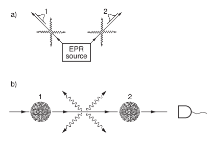
Figure 1: Illustration of continuous variable systems sharing entanglement between two light pulses (panel (a)) (see, e.g., Furusawa et al. (1998)), and between two macroscopic atomic gases (panel (b)) (see, e.g., Julsgaard et al. (2001)). The losses in the transmision lines carrying the entanglement to large distances is indicated by the wiggly curves emerging from the transmission lines.

In theory Duan et al. (2000) and experiment Julsgaard et al. (2001), entanglement between two trapped atomic gases is generated when the atoms are probed by off-resonant light (effective Faraday rotation interaction), and the transmitted probe light is monitored by homodyne detection. In Fig. 1(b) we display the situation we are concerned with. We imagine the gases to be at a large distance $L$ from each other and that there is a loss of $\epsilon$ in the light intensity between the two gases. Figure 1(a) illustrates the alternative situation where the entanglement is shared between two light beams propagating from an EPR source Braunstein and Kimble (1998); Furusawa et al. (1998); Kim and Lee (2001); Chizhov et al. (2002). In the present work we are primarily concerned with the system in panel (b), and the setup in (a) with entangled photons serves as a reference.

It is an interesting observation, that the no-distillation theorem precludes us from establishing several such entangled ensemble pairs and concentrating the entanglement into a single system, whereas during the optical probing of the atomic samples, the atomic entanglement is indeed increasing due to the sequential transmission of more and more segments of the light beam, which are also continuous variable quantum systems. It is accordingly not clear if the entanglement achievable in a single pair of atomic ensembles is fundamentally limited by loss and if so, what is its maximum value. We shall answer this question by direct computation of the state resulting from various measurement schemes.

The paper is organized as follows. In Sec. II, we introduce the measure of entanglement to be used throughout this work. In Sec. III, we recall the Gaussian covariance matrix analysis of the continuous variable systems. In Sec. IV we consider the atomic system (Fig. 1(b)) in the asymmetric case where light is sent in the direction from gas ’1’ to gas ’2’, only. In Sec. V we consider a symmetrized setup with light being sent in both directions. In Sec. VI we quantify the degree of entanglement that can be obtained in the two systems. In Sec. VII, we conclude with a discussion of the usefulness of the generated entanglement for teleportation with continuous quantum variables.

II Measures of entanglement

We are concerned with Gaussian continuous quantum variables systems. A Gaussian state for a vector of variables ${\bm{y}}=(y_{1},y_{2},\dots,y_{n})$ is fully characterized by its mean value vector $\bm{m}$ and its covariance matrix $\bm{\gamma}$ with entrance $ij$ given by $\gamma_{ij}=2\text{Re}\langle(y_{i}-\langle y_{i}\rangle)(y_{j}-\langle y_{j}\rangle)$. The degree of entanglement of a bipartite Gaussian state is therefore also characterized by its covariance matrix.

In our calculations below we are concerned with a two-mode covariance matrix which in a local ($x_{1},p_{1},x_{2},p_{2})$ basis of canonical conjugate variables reads

$$\gamma_{12}=\left(\begin{array}[]{cccc}v_{x_{1}}&0&c_{x}&0\\ 0&v_{p_{1}}&0&c_{p}\\ c_{x}&0&v_{x_{2}}&0\\ 0&c_{p}&0&v_{p_{2}}\\ \end{array}\right),$$ (5)

with $v_{x_{j}}=2\text{Var}(x_{j})$, $v_{p_{j}}=2\text{Var}(p_{j})$, and correlations $c_{\alpha}$, $(\alpha=x,p)$. To quantify the entanglement of such a state, we consider the logarithmic negativity Vidal and Werner (2002); Audenaert et al. (2002), $-\sum_{k=1}^{4}\log_{2}[\text{min}(1,|\lambda_{k}|)]$, which is calculated from the eigenvalues $\lambda_{k}$ of $i\sigma^{-1}\gamma_{12}^{T_{1}}$, where $\gamma_{12}^{T_{1}}$ is the partial transpose of $\gamma_{12}$ obtained by multiplying all entrances in $\gamma_{12}$ coupling $p_{1}$ and other observables by $-1$ (i.e., $c_{p}\rightarrow-c_{p}$ in (5)), and where $\sigma_{jk}=-i[y_{j},y_{k}]$ is the matrix specifying the commutators between our $x$ and $p$ variables. Here and throughout, $\hbar=1$. For a matrix of the above form, we find $|\lambda_{1}|=|\lambda_{2}|$ and $|\lambda_{3}|=|\lambda_{4}|$ and only one, say $|\lambda|$ of these norms may be smaller than unity and hence contribute to the measure of entanglement. We label this quantity $N=|\lambda|$, and the logarithmic negativity is then given by $-\log_{2}(N)$. The negativity $N$ is an analytical but lengthy expression of the elements of (5), and we will return to special cases in Sec. V.

In our analysis we shall also encounter the symmetric two-mode Gaussian state with covariance matrix

$${\bm{\gamma}}_{12}=\left(\begin{array}[]{cccc}n&0&k&0\\ 0&n&0&-k\\ k&0&n&0\\ 0&-k&0&n\\ \end{array}\right).$$ (10)

Now, $|\lambda_{1}|=|\lambda_{2}|=|n-k|$, $|\lambda_{2}|=|\lambda_{4}|=|n+k|$ and the negativity $N$ reduces to the quantity $\Delta=\text{Var}(x_{1}-x_{2})=\text{Var}(p_{1}+p_{2})$ known as the EPR uncertainty Giedke et al. (2003). We are interested in the case of entangled symmetric states where

$$N=\Delta=n-k,$$ (11)

and $N\in(0;1]$.

Since the logarithm in the evaluation of $-\log_{2}(N)$ is a monotonic function it is sufficient to consider the argument $N$ $(\Delta)$ in order to quantify the degree of entanglement for two-mode Gaussian states.

III Gaussian covariance formulation

First, as a reference, we study the influence of loss on the entangled fields of photons leaving an EPR-source (Fig. 1(a)). The entanglement in these fields is maximized when the entangled photons travel equal distances $L/2$ so the EPR-source is placed in the center of the transmission lines. For this symmetric setup, the covariance matrix $\gamma_{\text{EPR}}$ of the two beams is given by Eq. (10) with initial values of $n$ and $k$ determined by the squeezing parameter $|\chi|$ for a pure squeezed state, i.e., $n=\cosh|\chi|$, $k=\sinh|\chi|$, and consequently, the initial EPR uncertainty is given by $\Delta_{0}=\exp(-2|\chi|)$. In line with our previous works Mølmer and Madsen (2004); Madsen and Mølmer (2004), we write $\Delta_{0}=1/r$, and refer to $r$ as the squeezing parameter. The loss $\epsilon^{\prime}$ along each arm changes the canonical $x$ variable according to $x\mapsto{\sqrt{1-\epsilon^{\prime}}}x+{\sqrt{\epsilon^{\prime}}}x_{\text{noise}}$, where $x_{\text{noise}}$ describes the loss-induced vacuum contribution. For the $p$ quadrature we likewise have $p\mapsto{\sqrt{1-\epsilon^{\prime}}}p+{\sqrt{\epsilon}^{\prime}}p_{\text{noise}}$. In terms of the covariance matrix $\gamma_{\text{EPR}}$ the mapping is $\gamma_{\text{EPR}}\mapsto(1-\epsilon^{\prime})\gamma_{\text{EPR}}+\epsilon^{\prime}I_{4}$, where $I_{4}$ is the $4\times 4$ identity matrix. Therefore $n\mapsto(1-\epsilon^{\prime})n+\epsilon^{\prime}$ and $k\mapsto(1-\epsilon^{\prime})k$, and the EPR uncertainty, after the transmission, reads $\Delta_{\text{EPR}}\mapsto(1-\epsilon^{\prime})\Delta_{0}+\epsilon^{\prime}$. To relate to the loss $\epsilon$ in the full transmission line we assume a uniform loss per propagation distance and hence $(1-\epsilon^{\prime})={\sqrt{1-\epsilon}}$, and the final result for the EPR correlation is

$$\Delta_{\text{EPR}}=1+{\sqrt{1-\epsilon}}(1/r-1)>1-{\sqrt{1-\epsilon}},$$ (12)

where the last expression is obtained in the limit of infinite squeezing $r\rightarrow\infty$. The smaller the $\Delta_{\text{EPR}}$, the higher the degree of entanglement.

We now turn to the case where off-resonant light probes two separated atomic gases. A continuous-wave light beam which is linearly polarized along the $x$ direction is sent through samples of atoms with two degenerate Zeeman levels each described by a Pauli spin operator ${\bm{\sigma}}_{j}$ $(j=1,2,\dots,N_{a}$) Julsgaard et al. (2001). As discussed in detail elsewhere Madsen and Mølmer (2006a), we describe the interaction and the measurement process in the time-domain. A continuous-wave light beam is divided into segments of duration $\tau$ and length $L=c\tau$ each of which is assumed to be short enough to be accurately described by a single mode of the electromagnetic field. The interaction with the atoms and the feedback due to measurement is in turn described by a succession of interactions with the individual beam segments. For coherent light and the initially polarized samples, the uncertainty relations for these variables are minimized, implying a Gaussian state. The interaction of the samples with the off-resonant light beam gives rise to a Faraday-rotation interaction between the macroscopic spin operator ${\bm{J}}=1/2\sum_{j=1}^{N_{a}}{\bm{\sigma}}_{j}$ of the atoms and the Stokes operator ${\bm{S}}$ of the light field.

With maximally polarized atomic samples along the $x$ and $-x$ direction, we have the classical relations $J_{x,1}=J_{x}=-J_{x,2}=N_{a}/2$ where the subscripts ‘1’ and ‘2’ refer to the two gases. We assume a large number of photons in the probe beam such that the $x$ component of the Stokes vector $S_{x}$ also can be treated classically. This leads to the introduction of the following vector of quantum operators

$${\bm{y}} = (x_{1},p_{1},x_{2},p_{2},x,p)^{T}$$

$$= (\frac{J_{y,1}}{\sqrt{J_{x}}},\frac{J_{z,1}}{\sqrt{J_{x}}},\frac{-J_{y,2}}{\sqrt{J_{x}}},\frac{J_{z,2}}{\sqrt{J_{x}}},\frac{S_{y}}{\sqrt{S_{x}}},\frac{S_{z}}{\sqrt{S_{x}}})^{T},$$

with canonical commutators for the three independent sets of modes. For a probe laser field propagating in the $y$ direction and being linearly polarized in the $x$ direction, the Faraday rotation interaction is $\propto J_{z,i}S_{z}$ ($i=1,2$) and explicitly in terms of the effective Gaussian variables for a light segment of duration $\tau$ it reads

$$H_{i}=\kappa_{\tau,i}p_{i}p,$$ (14)

where $\kappa_{\tau,i}$ is the effective coupling constant $\kappa_{\tau,i}\propto\sqrt{N_{a}N_{ph}}$ where $N_{ph}$ is the number of photons in each segment. A polarization rotation measurement on the optical beam, i.e., a measurement of the $x$ variable of the probe light preserves the Gaussian character of the states and likewise does the bilinear Hamiltonian of Eq. (14).

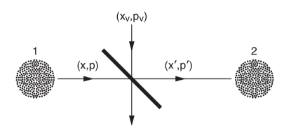
Figure 2: A beam splitter is used to model the effect of loss of light intensity $I\rightarrow(1-\epsilon)I$ through the transmission line on the $(x,p)$ variables of the field. The output or detector modes $(x^{\prime},p^{\prime})$ are determined by $x^{\prime}={\sqrt{1-\epsilon}}x+{\sqrt{\epsilon}}x_{v}$ and $p^{\prime}={\sqrt{1-\epsilon}}p+{\sqrt{\epsilon}}p_{v}$ (see text).

In previous work, the effects of loss of atomic spin polarization and absorption of light within the atomic clouds were investigated Madsen and Mølmer (2004); Sherson and Mølmer (2005). Here we focus on the loss associated with the light traveling from one gas to the other. This loss is partly in the transmission line and partly in the in-coupling devices connecting light to the atomic gas. The loss is modeled by a reduction ($1-\epsilon$) in the intensity in the probe beam along the transmission line. We model this loss by a beam splitter which mixes the incoming fields $x=(a+a^{\dagger})/\sqrt{2}$, $p=(a-a^{\dagger})/(i\sqrt{2})$ with vacuum fields $x_{v}$, $p_{v}$ (see Fig. 2). The beam splitter leads to a mixing of the operators of the incoming and the vacuum light modes $a\mapsto a^{\prime}=\sqrt{1-\epsilon}a+i\sqrt{\epsilon}a_{v}$, $a^{\dagger}\mapsto{a^{\dagger}}^{\prime}=\sqrt{1-\epsilon}a^{\dagger}-i\sqrt{\epsilon}a_{v}^{\dagger}$ where a prime denotes the operators of the modes after the passage of the beam splitter. From these relations which apply to each polarization component of the light field, and from the definitions of the Stokes vector components $S_{x}=a^{\dagger}_{x}a_{x}/2$, $S_{y}=(a^{\dagger}_{+}a_{-}-a^{\dagger}_{-}a_{+})/(2i)$, $S_{z}=(a_{+}^{\dagger}a_{+}-a^{\dagger}_{-}a_{-})/2$, the relations between the input and the primed output modes are easily determined. For the variables defined in Eq. (III), we find

$$\left(\begin{array}[]{c}p\\ p_{v}\\ \end{array}\right)=\left(\begin{array}[]{cc}\sqrt{1-\epsilon}&-\sqrt{\epsilon}\\ \sqrt{\epsilon}&\sqrt{1-\epsilon}\\ \end{array}\right)\left(\begin{array}[]{c}p^{\prime}\\ p^{\prime}_{v}\\ \end{array}\right),$$ (21)

and similarly for the $x$ variables.

The Hamiltonian describing the system when $x$-polarized light propagating in the $y$ direction is transmitted through the two gases is $H=\kappa_{\tau,1}p_{1}p+\kappa_{\tau,2}p_{2}p^{\prime}$. We note that the coupling strength to the second gas is reduced due to the loss of light intensity along the transmission line, $\kappa_{\tau,2}=\sqrt{1-\epsilon}\kappa_{\tau,1}$. We denote $\kappa_{\tau}=\kappa_{\tau,1}$, and use Eq. (21) to express the interaction Hamiltonian in the output modes $(x^{\prime},p^{\prime},x_{v}^{\prime},p_{v}^{\prime})$

$$H=\kappa_{\tau}\sqrt{1-\epsilon}(p_{1}+p_{2})p^{\prime}-\kappa_{\tau}\sqrt{\epsilon}p_{1}p_{v}^{\prime}.$$ (22)

The atomic $p_{1}$ and $p_{2}$ variables are coupled with equal strength to the output mode $p^{\prime}$, but the output vacuum noise term couples exclusively to $p_{1}$.

The Gaussian variables

$${\bm{y}}=(x_{1},p_{1},x_{2},p_{2},x^{\prime}_{v},p^{\prime}_{v},x^{\prime},p^{\prime})^{T},$$ (23)

describe conveniently the system with transmission loss. The time-evolution of the operators $y_{i}$ in ${\bm{y}}$ is described by Heisenberg’s equations of motion, $i\partial_{t}y_{i}=[y_{i},H]$. The evolution from $t$ to $t+\tau$ is then determined by the equation

$${\bm{y}}(t+\tau)=S{\bm{y}}(t),$$ (24)

with $S$ fixed by the Heisenberg equation and given in terms of the coupling $\kappa_{\tau}$ and the loss $\epsilon$. Per definition of the covariance matrix it follows that

$${\bm{\gamma}}(t+\tau)=S{\bm{\gamma}}(t)S^{T}.$$ (25)

Since the vacuum output components $x_{v}^{\prime},p_{v}^{\prime}$ describe loss, we should discard them after the interaction, which simply amounts to removing the corresponding rows and columns from $\gamma$, which then becomes a $6\times 6$ matrix.

We probe the system by measuring the Faraday rotation of the probe field, i.e., by measuring the light field observable $x^{\prime}$. The light field is correlated with the atomic samples and therefore this measurement will change the atomic state of the system. We denote the covariance matrix before interaction and detection of light by

$${\bm{\gamma}}=\left(\begin{array}[]{cc}A&C\\ C^{T}&B\\ \end{array}\right),$$ (28)

where the $4\times 4$ matrix $A$ describes the atomic systems, the $2\times 2$ matrix $B$ the output photon field, and the $4\times 2$ matrix $C$ the correlations between the field part of the system that is subject to direct measurement and the atomic part that only feels the measurement-induced back-action. An instantaneous measurement of $x^{\prime}$ transforms $A$ as Giedke and Cirac (2002); Fiurášek (2002); Eisert and Plenio (2003); Madsen and Mølmer (2006a)

$$A\mapsto A^{\prime}=A-C(\pi B\pi)^{-}C^{T},$$ (29)

where $\pi=\text{diag}(1,0)$ and where $(\cdot)^{-}$ denotes the Moore-Penrose pseudo-inverse. The other parts of the covariance matrix transform as $B\mapsto{\mathbb{I}}_{2\times 2}$, $C\mapsto 0_{4\times 2}$ since a new light segment is used in every measurement.

In Eq. (29), the change in $A$ is proportional to $\kappa_{\tau}^{2}$ which is proportional to the number of photons in the segment of duration $\tau$, and therefore proportional to $\tau$. We may then consider the update of the matrix $A$ in the limit of infinitesimally time steps and obtain a non-linear differential equation with coupling constant, $\kappa^{2}=\kappa_{\tau}^{2}/\tau$.

IV Asymmetric probing with squeezed light

Recently, we investigated the output field of an optical parametric amplifier Petersen et al. (2005a) and formulated a Gaussian theory in the time-domain that consistently described the squeezing of the fields for probing times longer than the inverse bandwidth of squeezing. In an application in precision magnetometry, we showed that essentially the same degree of squeezing and precision could be obtained as in the ultra-broadband squeezing case where the squeezing is just described by the squeezing parameter $r$. In the asymmetric case the two gases are subject to the interaction (22), and the squeezed light is described by a covariance matrix $\text{diag}(1/r,r)$, which in the output modes leads to $T\text{diag}(1,1,1/r,r)T^{-1}$ where $T$ describes the transformation from $(x_{v},p_{v},x,p)$ to $(x_{v}^{\prime},p_{v}^{\prime},x^{\prime},p^{\prime})$ (see Eq. (21)). The atomic covariance matrix for the two gases is denoted by $\gamma_{12}$ as in Eq. (1). We consider the continuous limit of the update formulas for $\gamma_{12}$ and obtain a non-linear Ricatti differential equation (see, e.g., Refs. Mølmer and Madsen (2004); Madsen and Mølmer (2004); Petersen et al. (2005b, a); Madsen and Mølmer (2006a)). The matrices in this equation describe squeezing of $p_{1}+p_{2}$, and noise introduced by the vacuum mode. The time-dependent covariance matrix which solves the Ricatti equation is on the form of Eq. (5) with

$$v_{x_{1}}=1+t\kappa^{2}(r+4\epsilon(1-r)+4\epsilon^{2}(r-1)),$$ (30a)

$$c_{x}=t(1-\epsilon)\kappa^{2}(r+2\epsilon(1-r)),$$ (30b)

$$v_{p_{1}}=\frac{t\kappa^{2}r(1-\epsilon)+(1-r)(1-\epsilon)+r}{2t\kappa^{2}r(1-\epsilon)+(1-r)(1-\epsilon)+r},$$ (30c)

$$c_{p}=-\frac{t\kappa^{2}r(1-\epsilon)}{2t\kappa^{2}r(1-\epsilon)+(1-r)(1-\epsilon)+r},$$ (30d)

$$v_{x_{2}}=1+t\kappa^{2}(1-\epsilon)(1+(1-r)(1-\epsilon)),$$ (30e)

$$v_{p_{2}}=\frac{t\kappa^{2}(1-\epsilon)r+(1-r)(1-\epsilon)+r}{2t\kappa^{2}(1-\epsilon)r+(1-r)(1-\epsilon)+r}.$$ (30f)

We use these expressions in Sec. VI to quantify the degree of entanglement between the two gases. We shall see that although some of these expressions diverge individually for large $t$, the logarithmic negativity approaches a constant value.

V Symmetric probing with squeezed light

We now turn to the symmetric case where equal amounts of noise is added to all four quadratures. The symmetric setup is obtained by sending light of different directions and polarizations through the two atomic samples, i.e., the gases are subject to the following sequence of effective interactions $H_{1}=\kappa_{\tau}\sqrt{1-\epsilon}(p_{1}+p_{2})p_{1}^{\prime}-{\sqrt{\epsilon}}p_{v1}^{\prime}\kappa_{\tau}p_{1}$, $H_{2}=\kappa_{\tau}\sqrt{1-\epsilon}(p_{1}+p_{2})p_{2}^{\prime}-{\sqrt{\epsilon}}p_{v2}^{\prime}\kappa_{\tau}p_{2}$, $H_{3}=\kappa_{\tau}\sqrt{1-\epsilon}(x_{1}-x_{2})x_{3}^{\prime}-{\sqrt{\epsilon}}x_{v3}^{\prime}\kappa_{\tau}x_{1}$, and $H_{4}=\kappa_{\tau}\sqrt{1-\epsilon}(x_{1}-x_{2})x_{4}^{\prime}+{\sqrt{\epsilon}}x_{v4}^{\prime}\kappa_{\tau}x_{2}$, where $p_{iv}^{\prime}$ and $x_{iv}^{\prime}$ are different vacuum modes. Each of these Hamiltonians leads to a propagation matrix $S$ via Heisenberg’s equations of motion. Tracing over all other degrees of freedom than those of the two atomic gases and adding the differential equations obtained for the four Hamiltonians above leads to a single Ricatti equation and if we probe with equal strengths and equal squeezing parameter (but $r\rightarrow 1/r$ when $p^{\prime}$ components are measured instead of $x^{\prime}$), the covariance matrix is of the symmetric form (10). The quantity $N=\Delta=n-k$ quantifies the degree of entanglement, and solves the equation

$$\partial_{t}\Delta=a-b\Delta^{2},$$ (31)

with growth rate for the noise

$$a=\kappa^{2}\epsilon(1-\epsilon+r\epsilon),$$ (32)

while the term driving the entanglement formation is given by

$$b=\frac{4\kappa^{2}r(1-\epsilon)}{1-\epsilon+r\epsilon}.$$ (33)

The solution to Eq. (31) with initial condition $\Delta(t=0)=1$ is found by quadrature and is given by

$$\Delta(t)=\frac{\cosh({\sqrt{ab}}t)+{\sqrt{\frac{a}{b}}}\sinh({\sqrt{ab}}t)}{\cosh({\sqrt{ab}}t)+{\sqrt{\frac{b}{a}}}\sinh({\sqrt{ab}}t)}.$$ (34)

In the presence of transmission line loss and squeezed light it follows that the steady-state value for the EPR uncertainty is

$$\Delta=\frac{1-\epsilon+r\epsilon}{2}\sqrt{\frac{\epsilon}{r(1-\epsilon)}}.$$ (35)

Since $\Delta$ must be less than unity for the two gases to be entangled, Eq. (35) shows that for unsqueezed probe light ($r=1$) it is possible to entangle the two gases only if $\epsilon<4/5$.

The minimum value of $\Delta$ (maximal entanglement) is

$$\Delta_{\text{min}}=\epsilon.$$ (36)

and is obtained for the optimal squeezing

$$r_{\text{opt}}=\frac{1-\epsilon}{\epsilon}.$$ (37)

This equation has as a consequence a property that at first sight seems surprising: for $\epsilon<1/2$ the minimum in $\Delta$ occurs for squeezed light ($r>1$) as expected, but for $\epsilon>1/2$ the minimum in $\Delta$ is obtained for antisqueezed light, $r<1$. This happens because the squeezed light input modes contribute to the undetected output mode which acts as a noise term $-{\sqrt{\epsilon}}p_{v}^{\prime}\kappa_{\tau}p_{1}$ on the first gas in Eq. (22). By Heisenberg’s equation of motion for $x_{1}$, we obtain from this part of the Hamiltonian the mapping $x_{1}\mapsto x_{1}^{\prime}=x_{1}-{\sqrt{\epsilon}}p_{v}^{\prime}\kappa_{\tau}$ which means that the added noise is determined by the variance $\epsilon\kappa^{2}\text{Var}(p_{v}^{\prime})=1/2\kappa^{2}\epsilon(1-\epsilon+r\epsilon)$ which is precisely half the factor entering the noise term in Eq. (32). When we probe with light that is squeezed (antisqueezed) in the $x$ quadrature, the $p$ quadrature is antisqueezed (squeezed) and the noise term is sensitive to the noise in this antisqueezed (squeezed) component

VI Quantifying the entanglement of the channel

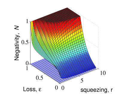
Figure 3: (Color online). Negativity at asymptotic times as a function of loss, $\epsilon$, and squeezing parameter $r\in[0.1;10]$ for the atomic asymmetric case where the light is only sent one way through the two samples, and where only the $x^{\prime}$ quadrature is probed.

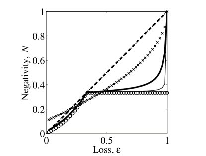
Figure 4: Optimal vales of the negativity for $r\in[0.1;10]$ at asymptotic times as a function of loss $\epsilon$ through the transmission line. The full curve corresponds to the case where the light is only sent one way through the two gases, and where only the $x^{\prime}$ quadrature is probed. The thin full curve corresponds to the case $r_{\text{min}}=0.01$. The long-dashed curve is for the symmetric case with $N=\epsilon$. The crossed curve is for the case of light emitted from an optical parametric oscillator (12) and the circles denote the asymptotic form of the full curve in the long-time and infinite-squeezing limit $r\gg 1$, $r\ll 1$, (38), (39).

For the asymmetric setup with light sent only one way through the samples, Fig. 3 shows a surface plot of the negativity $N$ for long probing times as a function of $\epsilon$ and $r$ for $r\in[0.1;10]$. The negativity $N$ is given by an analytical but very lengthy expression composed of sums of products of the variances and covariances from (30a)-(30f).

The results are summarized and compared with the symmetric interaction case and the EPR fields in Fig. 4. For a given loss, the full curve shows the optimum negativity from Fig. 3 assuming physical limits to the available squeezing $r_{\text{min}}=0.1$, $r_{\text{max}}=10$. The thin full curve shows the corresponding result for $r_{\text{min}}=0.01$, and the open circles show the results obtained with infinite squeezing: For losses less than $1/3$ and in the limit of infinite squeezing ($r\gg 1$) we obtain

$$N=\frac{\epsilon}{2-3\epsilon}.$$ (38)

For arbitrarily high losses, we find surprisingly that the negativity approaches a constant for antisqueezed light ($r\ll 1$)

$$N=1/3,$$ (39)

and we find that at the particular loss of $\epsilon=1/3$, $N=1/3$ for all values of the squeezing parameter, $r$. These results mean that no matter the loss it is always possible (assuming that the appropriate squeezed probe light source is available) to entangle the two gases to a high level.

The crossed curve is given by Eq. (12) for the symmetric EPR light source operated at a finite degree of squeezing $r=r_{\text{max}}=10$. The long-dashed curve describes the minimum value of $N$ for the symmetric atomic case (maximum entanglement) $N=\Delta_{\text{min}}=\epsilon$ obtained by the optimal squeezing of Eq. (37).

From Fig. 4 we see that for small loss and finite squeezing the light-atom system leads to higher entanglement than achievable with the EPR light source for the same degree of squeezing. For the asymmetric atom-light case we see from the full curve in Fig. 4 that the atom-light setup leads to a higher degree of entanglement than the EPR light source except in a narrow range around $\epsilon=1/3$. In particular for losses exceeding $\sim$ 40 %, the asymmetric setup presents an efficient way to generate a high and constant degree of entanglement.

VII Discussion

In summary, we have studied the effects of (light) losses on the achievable entanglement between two locations coupled by a lossy transmission line. We characterize the entanglement by the argument $N$ of the logarithmic negativity $-\log_{2}(N)$. The entanglement of atomic samples by optical probing is experimentally interesting because it works with classical optical sources and because the entangled states are stored in stationary media for potential later use. If only coherent light is available, the entanglement obtained with light being sent in both directions between the gases and with probing of suitable combinations of both the $x$ and $p$ atomic variables yields $N=\sqrt{\epsilon/(4-4\epsilon)}$, and the gases become entangled as long as the losses are below 80 %. When squeezed light is available, we both have the possibility to simply prepare and send entangled light pulses over the transmission channel and we may use the squeezed light to improve the atomic probing schemes. For low losses, and with no limits to the degree of squeezing, the mere emission of entangled light pulses yields the largest entanglement, but if the degree of available optical squeezing is limited, it becomes advantageous to use probed atomic samples, and, quite surprisingly we showed that for large losses, a one-way probing scheme with anti-squeezed light leads to a finite negativity $N=1/3$ and a logarithmic negativity as large as $\log_{2}(3)$ for any value of the loss. When the loss approaches unity, the required degree of anti-squeezing and probing time get larger, but as shown in Fig. 4., realistic squeezing levels suffice to give surprisingly small $N$ for large losses.

Entangled states have been proposed for various quantum communication tasks, and since losses set a practical limit on the distance over which these tasks can be carried out, a scheme that attains high entanglement despite losses is of course interesting. To investigate if our entanglement is useful, we present a brief analysis of the achievements of the entangled gases for continuous variables teleportation Braunstein and Kimble (1998). We have recently presented a general analysis of fidelities for Gaussian state transformations, including teleportation  Madsen and Mølmer (2006b), and for an entangled channel of the form (3), we reproduced the known fidelity for teleportation of an unknown coherent state

$$F=\frac{1}{1+n-k}=\frac{1}{1+\Delta}.$$ (40)

This result applies to the case of symmetric probing, and with optimum use of squeezed probing light (36) the fidelity gets as high as

$$F^{\text{opt}}=\frac{1}{1+\epsilon},$$ (41)

approaching the classical limit of $F_{\text{classical}}=1/2$ Hammerer et al. (2005) when the whole light field is lost.

The entangled state obtained from the asymmetric probing can also be applied in the Braunstein-Kimble teleportation protocol, in which case the fidelity is expressed in terms of the variances of the non-local variables of the entangled channel $p_{+}=(p_{1}+p_{2})/{\sqrt{2}}$ and $x_{-}=(x_{1}-x_{2})/{\sqrt{2}}$:

$$F=\frac{1}{\sqrt{(1+2\text{Var}(p^{(12)}_{+}))(1+2\text{Var}(x^{(12)}_{-}))}}.$$ (42)

The theory in Sec. IV provides the values $\text{Var}(p^{(12)}_{+})=1/(2(1+\beta t))$, $\text{Var}(x_{-}^{(12)}=(1+\alpha t)/2$ with $\beta=2(1-\epsilon)r\kappa^{2}/(1+r\epsilon-\epsilon)$ and $\alpha=\kappa^{2}\epsilon(1+r\epsilon-\epsilon)/2$, and instead of applying the protocol directly we suggest to locally anti-squeeze the $p$’s, and hence $p^{(12)}_{+}$, and squeeze the $x$’s, and hence $x^{(12)}_{-}$, so that $\text{Var}(p^{(12)}_{+})\rightarrow s\text{Var}(p^{(12)}_{+})$, and $\text{Var}(x^{(12)}_{-})\rightarrow\text{Var}(x^{(12)}_{-})/s$. The maximum value of (42) is obtained for $s=\sqrt{\text{Var}(x^{(12)}_{-})/\text{Var}(p^{(12)}_{+})}$,

$$F=\frac{1}{1+2\sqrt{\frac{1+\alpha t}{1+\beta t}}}\rightarrow\frac{1}{1+2\sqrt{\alpha/\beta}}\ \ (t\rightarrow\infty).$$ (43)

This expression is always less than or equal to $1/(1+\epsilon)$, the optimum in the case of symmetric probing (41) with squeezed light, and equality is obtained for probing with squeezed/anti-squeezed light with a finite squeezing factor, $r=(1-\epsilon)/\epsilon$, which is incidentally also the optimal optical squeezing in the case of symmetric probing. For large $\epsilon$, e.g., $90\%$, this value of $r$ does indeed lead to significant entanglement, cf. Fig.4, but the teleportation fidelity behaves ”normally” and approaches the classical value of $1/2$ when $\epsilon\rightarrow 1$. The surprisingly high entanglement does not provide a scheme for high fidelity teleportation!

We note that we have not really proven that we made optimum use of the entangled state by the straightforward use of the Braunstein-Kimble protocol, but we can give an independent argument for why (41) must be the optimum teleportation fidelity in the case of the asymmetric probing scheme: Imagine a modified physical setup where the transmission line and the second gas of our analysis is replaced by a loss less beam splitter arrangement and $M$ separate gases, which each receive a fraction $1/M$ of the field after transmission through the first gas. Any one of these gases will become entangled with the first gas as described by the above theory, if we identify the transmitted fraction $1-\epsilon$ with $1/M$. The teleportation of an unknown coherent state is accomplished by performing a joint measurement on the incident state and the first gas, and communicating the outcome to the other site, where a local operation on the quantum system establishes the output state. Since we share the entangled state with $M$ different sites, we are thus able to teleport the same state to $M$ different sites, i.e., produce $M$ approximate clones of the incoming state. The fidelity for each of these clones, however, has been shown by a different argument to be limited by the value $M/(2M-1)=1/(1+\epsilon)$ Cerf and Iblisdir (2000), which therefore must also be the upper limit of our teleportation fidelity.

In conclusion, without violating fundamental results on the achievements of distillation, purification and cloning of Gaussian states, we have identified a protocol, that leads to finite entanglement between systems which are coupled by even very lossy transmission lines. If the probing field is split and distributed evenly between a number of partners, our analysis identifies instead a new kind of ”entanglement polygamy”, where a single system can share finite entanglement with an unlimited number of other systems. Unlike a recent proposals for multi-partite Gaussian GHZ-type states Adesso and Illuminati (2005), where the entanglement can be concentrated and used for high-fidelity teleportation between any pair by measurements on all the other systems, our entanglement is already sizable, but not correspondingly useful for teleportation. The logarithmic negativity has been criticized for not always giving a reliable characterization of the entanglement of quantum systems. In our case, however, we have observed that also the more involved Gaussian entanglement of formation Wolf et al. (2004) is finite for large losses. Rather than demonstrating a weakness of specific entanglement measures, we believe that the present study is a contribution to our discovery of different varieties of useful and, possibly, useless entanglement.