On the statistics of quantum expectations
for systems in thermal equilibrium

Abstract

The recent remarkable developments in quantum optics, mesoscopic and cold atom physics have given reality to wave functions. It is then interesting to explore the consequences of assuming ensembles over the wave functions simply related to the canonical density matrix. In this note we analyze a previously introduced distribution over wave functions which naturally arises considering the Schrödinger equation as an infinite dimensional dynamical system. In particular, we discuss the low temperature fluctuations of the quantum expectations of coordinates and momenta for a particle in a double well potential. Our results may be of interest in the study of chiral molecules.

1 Introduction

Quantum statistical mechanics is usually based on the canonical ensemble described by the density matrix $\bm{\rho}_{\beta}=Z^{-1}\exp(-\beta\mathbf{H})$, with $Z=\mathrm{tr}\exp(-\beta\mathbf{H})$. In his celebrated book on statistical thermodynamics, Schrödinger S remarked that “this assumption is irreconcilable with the very foundations of quantum mechanics” because microsystems in general will not be in an energy eigenstate. The reason why this assumption can be accepted is that a more consistent attitude “leads to the same thermodynamical results”. The more consistent attitude, according to Schrödinger, consists in introducing an ensemble over the states (wave functions) in which one attributes the same probability to all the highly degenerate energy states of a macroscopic system. He then shows that for a subsystem one expects the canonical ensemble to be approximately correct. In a recent paper GLTZ Schrödinger’s statement has been substantially strengthened. See also Bloch .

In the last decade the remarkable developments in quantum optics, mesoscopic and cold atom physics have given reality to wave functions. It is enough to think of the many realizations of “Schrödinger cats” or of coherent states. It is then interesting to explore the consequences of assuming ensembles over the wave functions simply related to the canonical density matrix. A guide in the choice of an ensemble is the observation that the Schrödinger equation, $i\partial_{t}\psi=H\psi$, and its complex conjugate can be considered as an infinite dimensional Hamiltonian system in the variables $\psi$ and $\psi^{*}$ with Hamiltonian $\langle\psi,\mathbf{H}\psi\rangle$. It is therefore natural to concentrate our attention on measures invariant under this dynamics. In Jona an ensemble over the wave functions was introduced, hereafter named Schrödinger-Gibbs (SG) ensemble, with formal measure

$$d\mu_{\mathrm{SG}}(\psi)=Z_{\mathrm{SG}}^{-1}e^{-\beta\langle\psi,\mathbf{H}\psi\rangle}\delta\left(1-\langle\psi,\psi\rangle\right)\prod d\psi,$$ (1)

where $\langle\cdot,\cdot\rangle$ is the usual scalar product in the Hilbert space. A simple calculation shows that in terms of (1) the canonical ensemble can be written

$$\bm{\rho}_{\beta}=\int|\psi\rangle\langle\psi|\left(\sum_{k}\delta(\psi-\psi_{k})\right)d\mu_{\mathrm{SG}}(\psi),$$ (2)

where $\psi_{k}$ are the unnormalized eigenstates of $\mathbf{H}$, assumed to have a discrete spectrum.

In Jona the motivation was to calculate the distribution of quantum expectation values of the operators $\mathbf{q}$ and $\mathbf{p}$ induced by the SG ensemble. A formula for such a distribution was found at low temperature and the wave functions giving the largest contributions were characterized in terms of an appropriate Legendre transform of the ground state energy of the system in an external field. These wave functions in the case of the harmonic oscillator are the usual coherent states and, by analogy, we shall adopt this name also in the general case.

The distribution for the expectation values $\langle\mathbf{q}\rangle$ and $\langle\mathbf{p}\rangle$ is different from that obtained with the usual quantum canonical ensemble. For example, in the latter case for reflection invariant systems $\langle\mathbf{q}\rangle$ does not fluctuate at all, a rather unphysical result.

In this paper, after recalling the main steps in Jona , we analyze in detail the case of a one-dimensional double well, which is an ubiquitous system in physics and deeply non classical at low energies. The result is a Gibbsian distribution of the expectation values $\langle\mathbf{q}\rangle$ and $\langle\mathbf{p}\rangle$ of the form $P(\langle\mathbf{q}\rangle,\langle\mathbf{p}\rangle)\simeq\exp\{-\beta[\langle\mathbf{p}\rangle^{2}/(2m)+V_{\mathrm{eff}}(\langle\mathbf{q}\rangle)]\}$, where $V_{\mathrm{eff}}(\langle\mathbf{q}\rangle)$ is an effective potential with a single minimum. This minimum is at zero for the symmetric double well or near the point where the ground state function is concentrated in the asymmetric case. This result may be of interest in connection with pyramidal molecules, like ammonia or other molecules potentially chiral. For these systems which are adequately described, as far as the inversion degrees of freedom are concerned, by a symmetric double well CJL ; JLPT , fluctuations of $\langle\mathbf{q}\rangle$ correspond to fluctuations of the electric dipole moment and could be in principle observable providing thereby a test of the statistical assumption (1).

2 Low temperature limit

We discuss first the harmonic oscillator defined by the Hamiltonian $\mathbf{H}=\mathbf{p}^{2}/2m+m\omega^{2}\mathbf{q}^{2}/2$. For this system the Heisenberg equations of motion of the canonical operators $\mathbf{q}$ and $\mathbf{p}$, namely $\dot{\mathbf{q}}=\mathbf{p}/m$ and $\dot{\mathbf{p}}=-m\omega^{2}\mathbf{q}$, bring to the $c$-number equations for the expectations

$$\dot{\langle\mathbf{q}\rangle} = \langle\mathbf{p}\rangle/m$$ (3)

$$\dot{\langle\mathbf{p}\rangle} = -m\omega^{2}\langle\mathbf{q}\rangle.$$ (4)

In the following, we will use the notation $\langle\mathbf{q}\rangle=q$ and $\langle\mathbf{p}\rangle=p$. The Hamiltonian flow (3-4) admits the canonical invariant measure $Z^{-1}\exp[-\beta H(q,p)]dqdp$, where $H(q,p)=p^{2}/2m+m\omega^{2}q^{2}/2$ and $\beta$ is a constant. We want to show that this result can be obtained from the formal SG-measure (1). The probability density of the expectation values $q$ and $p$ is given by

$$P(q,p)=\int\delta\left(q-\langle\psi,\mathbf{q}\psi\rangle\right)\delta\left(p-\langle\psi,\mathbf{p}\psi\rangle\right)d\mu_{\mathrm{SG}}(\psi).$$ (5)

The Fourier transform of the above expression can be evaluated exactly and transforming back to the variables $q$ and $p$ one finds

$$P(q,p)=\frac{\beta\omega}{2\pi}\exp[-\beta(p^{2}/2m+m\omega^{2}q^{2}/2)].$$ (6)

It is interesting to determine which kind of wave functions contribute mostly to $P(q,p)$ in the low temperature regime $\beta\to\infty$. To this purpose we have to minimize $\langle\psi,\mathbf{H}\psi\rangle$ with the three constraints $\langle\psi,\psi\rangle=1$, $\langle\psi,\mathbf{q}\psi\rangle=q$, and $\langle\psi,\mathbf{p}\psi\rangle=p$. Once more the calculation can be performed exactly and one finds that the minimizing wave functions are

$$\psi_{q,p}(x)=\left(\frac{m\omega}{\pi\hbar}\right)^{1/4}\exp\left[\frac{i}{\hbar}px-\frac{1}{2}\frac{m\omega}{\hbar}(x-q)^{2}\right],$$ (7)

i.e. the harmonic oscillator coherent states.

We wish now to generalize the above results to systems described by Hamiltonians $\mathbf{H}=\mathbf{p}^{2}/2m+V(\mathbf{q})$ with non quadratic potentials $V(\mathbf{q})$. In that case, the density $P(q,p)$ cannot be evaluated exactly, however, we can estimate it for low temperatures. In fact, for $\beta$ large from steepest descent we have

$$P(q,p) \simeq \exp[-\beta\langle\psi_{q,p},\mathbf{H}\psi_{q,p}\rangle],$$ (8)

where $\simeq$ means asymptotic logarithmic equality and $\psi_{q,p}$ is a normalized state which minimizes the expectation of $\mathbf{H}$ with the constraints $\langle\psi_{q,p},\mathbf{q}\psi_{q,p}\rangle=q$ and $\langle\psi_{q,p},\mathbf{p}\psi_{q,p}\rangle=p$. First we get rid of the latter constraint by putting

$$\psi_{q,p}(x)=\exp(ipx/\hbar)\phi_{q}(x)$$ (9)

with $\langle\phi_{q},\phi_{q}\rangle=1$. The state $\phi_{q}$ is determined as the ground state $\phi_{\lambda(q)}^{0}$ of the eigenvalue problem

$$\left(\mathbf{H}+\lambda\mathbf{q}\right)\phi_{\lambda}=E_{\lambda}\phi_{\lambda},$$ (10)

solved self-consistently with the Lagrange multiplier $\lambda=\lambda(q)$ specified by the condition

$$\langle\phi_{\lambda}^{0},\mathbf{q}\phi_{\lambda}^{0}\rangle=q.$$ (11)

If $E^{0}_{\lambda(q)}$ is the eigenvalue associated to the ground state $\phi_{\lambda(q)}^{0}$, we have

$$\langle\psi_{q,p},\mathbf{H}\psi_{q,p}\rangle=\frac{p^{2}}{2m}+\langle\phi_{q},\mathbf{H}\phi_{q}\rangle=\frac{p^{2}}{2m}+E^{0}_{\lambda(q)}-\lambda(q)q.$$ (12)

In conclusion, we obtain

$$P(q,p) \simeq \exp\left[-\beta\left(p^{2}/2m+V_{\mathrm{eff}}(q)\right)\right],$$ (13)

where the effective potential $V_{\mathrm{eff}}(q)=E^{0}_{\lambda(q)}-\lambda(q)q$ is evaluated by solving the nonlinear eigenvalue problem (10-11). In analogy to the harmonic oscillator case, we call $\psi_{q,p}(x)=\exp(ipx/\hbar)\phi^{0}_{\lambda(q)}(x)$ coherent states.

On the other hand, in the canonical ensemble for the probability density of the expectations of $q$ and $p$ we immediately obtain

$$P(q,p)=Z^{-1}\sum_{k}e^{-\beta E_{k}}\delta(q-q_{k})\delta(p),$$ (14)

where $Z=\sum_{k}e^{-\beta E_{k}}$ and $q_{k}=\langle\varphi_{k},\mathbf{q}\varphi_{k}\rangle$. Here, $\varphi_{k}$ are the normalized eigenstates of $\mathbf{H}$ with eigenvalues $E_{k}$. In particular, for system invariant under reflection we have $P(q,p)=\delta(q)\delta(p)$.

3 Double well systems

We consider a particle in a symmetric double well potential of the form

$$V(\mathbf{q})=W_{0}(\mathbf{q}^{2}-x_{0}^{2})^{2}$$ (15)

and solve numerically the nonlinear eigenvalue problem (10-11) to obtain the effective potential $V_{\mathrm{eff}}(q)$. This task is accomplished efficiently by the selective relaxation algorithm PT . The results are reported in Fig. 1. We expect that in this problem one can approximate the original Hamiltonian $\mathbf{H}$ with a two-state Hamiltonian restricted to the lowest two eigenfunctions of $\mathbf{H}$ corresponding to the splitting of the ground state induced by tunneling. For this reason, we report in Fig. 1 both the exact numerical calculations and the two-state approximation. In the latter case, the effective potential can be evaluated analytically and one finds

$$V_{\mathrm{eff}}(q)=\frac{E_{2}+E_{1}}{2}-\frac{E_{2}-E_{1}}{2}\sqrt{1-\left(\frac{q}{d}\right)^{2}},$$ (16)

where

$$d=(\varphi_{1},\mathbf{q}\varphi_{2})$$ (17)

and $\varphi_{1}$ and $\varphi_{2}$ are the lowest eigenstates of $\mathbf{H}$ with eigenvalues $E_{1}$ and $E_{2}$, respectively. Figure 1 shows that the two-state approximation is rather good and, in fact, it becomes more and more accurate in the semiclassical limit, for example by increasing the value of the mass $m$.

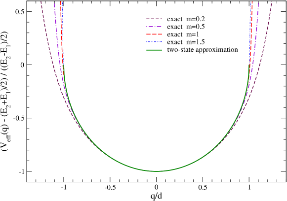
Figure 1: Rescaled effective potential $(V_{\mathrm{eff}}(q)-(E_{2}+E_{1})/2)/((E_{2}-E_{1})/2)$ as a function of the rescaled expectation $q/d$ evaluated numerically for the double well potential (15) with different values of the mass $m$. The solid thick line represents the two-state approximation (16). For the other parameters we set, in all cases, $\hbar=1$, $x_{0}=1.5$, and $W_{0}=1$. The values of $E_{1}$, $E_{2}$, and $d$ used in the rescaling have been evaluated numerically and are: $E_{1}=3.415753$, $E_{2}=4.877688$, and $d=1.158335$ for $m=0.2$, $E_{1}=2.582908$, $E_{2}=2.865508$, and $d=1.268715$ for $m=0.5$, $E_{1}=1.970442$, $E_{2}=2.012262$, and $d=1.353385$ for $m=1$, $E_{1}=1.64383345$, $E_{2}=1.65329839$, and $d=1.38670188$ for $m=1.5$.

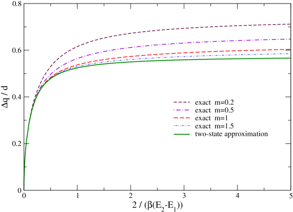
Figure 2: Rescaled fluctuation $\Delta q/d$ as a function of the rescaled temperature $2/(\beta(E_{2}-E_{1}))$ evaluated numerically for the double well potential (15) with different values of the mass $m$ as in Fig. 1. The solid thick line is the approximated result obtained from $V_{\mathrm{eff}}$ given by Eq. (16).

In the two-state approximation the coherent states $\psi_{q,p}$ are given by

$$\psi_{q,p}(x)=e^{ipx/\hbar}\left[c_{1}(q)\varphi_{1}(x)+c_{2}(q)\varphi_{2}(x)\right],$$ (18)

where

$$c_{1}(q)=\frac{1}{\sqrt{2}}\sqrt{1-q/d}\qquad c_{2}(q)=\frac{1}{\sqrt{2}}\sqrt{1+q/d}.$$ (19)

In the semiclassical limit the difference $E_{2}-E_{1}$ tends to zero exponentially and the effective potential becomes flat between $\pm x_{0}$. In this limit $d\to x_{0}$. This reflects the fact that the two levels become equiprobable for low temperatures so that any superposition of the corresponding states has the same probability. In the same limit, the dispersion $\Delta q=(\overline{q^{2}}-\overline{q}^{2})^{1/2}$ tends to $x_{0}/\sqrt{3}$ as it is apparent in Fig. 2.

References

- (1) E. Schrödinger, Statistical Thermodynamics (Cambridge University Press, Cambridge, England, 1952).
- (2) S. Goldstein, J. L. Lebowitz, R. Tumulka and N. Zanghì, Phys. Rev. Lett. 96, 050403 (2006).
- (3) F. Bloch and J. D. Walecka, Fundamentals of Statistical Mechanics: Manuscripts and Notes of Felix Bloch, Standford University Press, 1989.
- (4) G. Jona-Lasinio, “Invariant Measures under Schrödinger evolution and quantum statistical mechanics,” in Stochastic Processes, Physics and Geometry: New Interplays. I: A Volume in Honor of Sergio Albeverio, edited by F. Gesztesy, H. Holden, J. Jost, S. Paycha, M. Röckner, and S. Scarlatti, Canadian Mathematical Society Conference Proceedings, Volume 28 (2000), pp. 239–242.
- (5) D. C. Brody and L. P. Hughston, J. Math. Phys. 39, 6502 (1998).
- (6) P. Claverie and G. Jona-Lasinio, Phys. Rev. A, 33, 2245 (1986).
- (7) G. Jona-Lasinio, C. Presilla, C. Toninelli Phys. Rev. Lett. 88, 123001 (2002).
- (8) C. Presilla and U. Tambini, Phys. Rev. E 52, 4495 (1995).