Non-Hermitian quantum mechanics: the case of bound state scattering theory

Abstract

Excited bound states are often understood within scattering based theories as resulting from the collision of a particle on a target via a short-range potential. We show that the resulting formalism is non-Hermitian and describe the Hilbert spaces and metric operator relevant to a correct formulation of such theories. The structure and tools employed are the same that have been introduced in current works dealing with PT-symmetric and quasi-Hermitian problems. The relevance of the non-Hermitian formulation to practical computations is assessed by introducing a non-Hermiticity index. We give a numerical example involving scattering by a short-range potential in a Coulomb field for which it is seen that even for a small but non-negligible non-Hermiticity index the non-Hermitian character of the problem must be taken into account. The computation of physical quantities in the relevant Hilbert spaces is also discussed.

1 Introduction

The standard formulation of quantum mechanics requires physical observables to be mathematically given in terms of Hermitian operators. In recent years theories with a non-Hermitian Hamiltonian have been receiving an increasing interest sparked by work in the field of PT-symmetric quantum mechanics [1]. PT-symmetric Hamiltonians are complex but nevertheless possess a real spectrum. The structure of PT-symmetric theories, initially suggested to hinge on the existence of a charge conjugation operator [2] has been clarified by showing [3] that the non-Hermitian Hamiltonians could be mapped to Hermitian ones, and therefore be fitted within the better-known framework of quasi-Hermitian operators [4]. The relevance of the non-Hermitian formulation for the description of physical systems is still being debated [5, 6, 7, 8].

In the present work we show that the effective Hamiltonians appearing in certain theories dealing with bound state scattering by a short-range potential are non-Hermitian. In this case the Hamiltonians are real and their non-Hermitian character stems from the boundary conditions obeyed by the eigenstates: on the one hand there is no physical asymptotic freedom (since the states are bound) and on the other the scattering solutions inside the short-range potential region do not exist. However contrarily to the situation in PT-symmetric problems, there is in principle an underlying Hermitian Hamiltonian, whose solutions are unknown in practice but whose existence may provide guiding rules when undertaking practical computations. We will see that the unambiguous formulation of bound state scattering sheds some light on issues regarding the physical relevance of non-Hermitian formulations of quantum mechanics. Let us mention that in the overwhelming majority of applications of the bound state scattering formalism to nuclear, atomic or molecular physics non-Hermitian issues have been downright ignored; this is unproblematic when non-Hermiticity is small (as is generally the case), but we will give an illustration in which ignoring the non-Hermitian nature of the scattering Hamiltonian brings in errors that can be directly attributed to the (inappropriate) use of the standard inner product.

We will first introduce bound state scattering theory and show why the scattering Hamiltonian is non-Hermitian in the ’physical’ Hilbert space $\mathcal{H}_{ph}$ (Sec 2). The quasi-Hermitian Hamiltonian will then be described by an expansion in terms of a biorthogonal basis, leading naturally to the definition of a new inner product and its associated Hilbert space $\mathcal{H}$ (Sec 3). In line with previous works on quasi-Hemitian operators, we will examine the relationship between the two Hilbert spaces $\mathcal{H}_{ph}$ and $\mathcal{H}$ in terms of the metric operator and further discuss the computation of physical results in $\mathcal{H}$ and $\mathcal{H}_{ph}$. In Sec 4, the formalism will be illustrated by carrying out the numerical calculation of an experimentally observable quantity (the autocorrelation function) in the particular case of short-range scattering in a Coulomb field. Our concluding remarks will be given in Sec 5.

2 Scattering description of excited bound states

Let $H^{e}$ be the exact Hamiltonian of the 2-particle scattering problem (in the center of mass; the physical situation most often considered is that of a light particle colliding on a massive compound target). We assume $H^{e}$ can be split as

$$H^{e}=H_{0}+V$$ (1)

where $V$ contains all the short range interactions between the particles. We further assume $H_{0}$ is spherically symmetric (in terms of the relative coordinate) and that short-range means that

$$V=\theta(r_{0}-r^{\prime})V\theta(r_{0}-r),$$ (2)

ie $V$ vanishes outside some small radius $r_{0}$ ($\theta$ is the step function). Therefore $H_{0}$ contains not only the kinetic and internal terms of the non-interacting particles, but also any long-range interaction between them. Let $E$ be the total energy; allowing for inelastic scattering $E$ is partitioned as

$$E=\varepsilon_{i}+\epsilon_{i}$$ (3)

where $\varepsilon_{i}$ and $\epsilon_{i}$ are the internal and the kinetic energy respectively (in the case of a massive target $\varepsilon_{i}$ depends on the internal states of the target whereas $\epsilon_{i}$ is the collision energy of the light particle). The eigenstates of $H_{0}$ are given by

$$\left|\phi_{i}(E)\right\rangle=\left|f_{i}(\epsilon_{i})\right\rangle\left|i(\varepsilon_{i})\right\rangle;$$ (4)

$f_{i}(\epsilon_{i},r)\equiv\left\langle r\right.\left|f_{i}(\epsilon_{i})\right\rangle$ is the eigenfunction of the radial part of $H_{0}$ whereas the ’target’ state $\left|i(\varepsilon_{i})\right\rangle$ includes all the other degrees of freedom, including the non-radial ones of the colliding particle (a handy notation given that the angular momenta of the particles are usually coupled). The target states are orthogonal, $\left\langle i\right|\left.j\right\rangle=\delta_{ij}$. Since we are dealing with bound states, $f_{i}(\epsilon_{i},r)$ vanishes at $0$ and $+\infty$ (whenever $E$ is an eigenvalue of $H_{0}$).

The label $i$ defines the scattering channel. In each channel the standing-wave solutions are given by the Lippmann-Schwinger equations of scattering theory as

$$\left|\psi_{i}^{e}(E)\right\rangle=\left|\phi_{i}(E)\right\rangle+G_{0}(E)K(E)\left|\phi_{i}(E)\right\rangle$$ (5)

where $G_{0}(E)$ is the principal-value Green’s function and $K$ the reaction (scattering) operator for standing waves linked to the familiar $S$ matrix by a Cayley transform [12]. The difference here with standard scattering theory is that the bound channels are included explicitly [9, 10, 11]. The consequences are that (i) $G_{0}(E)$ has no poles – it is modified [9] relative to the usual resolvent by including a term (solution of the homogeneous equation) that has poles at the eigenvalues of $H^{e}$ so that overall $G_{0}(E)$ has no poles (but diverges radially) ; (ii) there is no asymptotic freedom: both $\left\langle r\right|\left.\phi_{i}(E)\right\rangle$ and $\left\langle r\right|\left.\psi_{i}^{e}(E)\right\rangle$ diverge at $r\rightarrow\infty$ for an arbitrary value of $E$; (iii) an eigenstate of $H^{e}$ cannot be given by a single channel solution of the form (5) but requires a superposition

$$\left|\psi^{e}(E)\right\rangle=\sum_{i}Z_{i}(E)\left|\psi_{i}^{e}(E)\right\rangle$$ (6)

where the expansion coefficients $Z_{i}(E)$ are determined by the asymptotic ($r\rightarrow\infty$) boundary conditions such that at the eigenvalues $\left\langle r\right|\left.\psi^{e}(E)\right\rangle$ vanishes at infinity.

Formally $H^{e}\left|\psi^{e}(E)\right\rangle=E\left|\psi^{e}(E)\right\rangle$ is satisfied as well as the usual properties for eigenstates of Hermitian operators, such as their orthonormality

$$\left\langle\psi^{e}(E_{1})\right|\left.\psi^{e}(E_{2})\right\rangle=\delta_{E_{1}E_{2}}$$ (7)

or the spectral decomposition theorem. However in practice the expansion of $G_{0}$ over the eigenstates of $H_{0}$ is intractable. Instead the radial part of $G_{0}$ is separated and the expansion over the energies reduced to the closed form $f_{i}(\epsilon_{i},r_{<})g_{i}(\epsilon_{i},r_{>})$; $g_{i}$ is a solution of the radial part of $H_{0}$ irregular at the origin (for arbitrary bound energies, both $f$ and $g$ exponentially diverge in the limit $r\rightarrow\infty$). Hence the closed form of the radial Green’s function only makes sense for $r>r_{0}$ (where $V$ vanishes). This is of course consistent with the scattering point of view: when $r<r_{0}$ we are inside the reaction zone and there is no scattering solution, whatever happens within the reaction zone being encoded in the phase-shifts. The wavefunction (6) outside the reaction zone becomes

$$\left\langle r\right.\left|\psi(E)\right\rangle=\sum_{i}Z_{i}(E)\left[f_{i}(\epsilon_{i},r)\left|i\right\rangle+\sum_{j}g_{j}(\epsilon_{j},r)\left|j\right\rangle K_{ji}\right]\qquad r>r_{0}$$ (8)

where $K_{ji}$ are the on-shell elements of the scattering matrix, which are assumed to be known.

It is important to note that the scattering eigenstate (8) is the part for $r>r_{0}$ of the exact solution $\left|\psi^{e}(E)\right\rangle$, and not an approximation to it. But within the scattering fomulation the ’inner’ part of $\left|\psi^{e}(E)\right\rangle$ for $r<r_{0}$ does not exist: all meaningful quantities are defined radially on $[r_{0},\infty[$. Indeed let us write

$$\left|\psi^{e}(E)\right\rangle=\theta(r-r_{0})\left|\psi(E)\right\rangle+\theta(r_{0}-r)\left|\psi_{inner}(E)\right\rangle$$ (9)

and let

$$H\equiv\sum_{E}E\left|\psi(E)\right\rangle\left\langle\psi(E)\right|$$ (10)

be the restriction of $H^{e}$ to the outer region $r>r_{0}$. $H$ is the only operator directly known from the solutions of the scattering problem. We have the following properties :

$$H=H^{+}$$ (11)

$$\left\langle\psi(E_{1})\right|\left.\psi(E_{2})\right\rangle=\delta_{E_{1}E_{2}}+\mu_{E_{1}E_{2}}(1-\delta_{E_{1}E_{2}})$$ (12)

$$H\left|\psi(E)\right\rangle\neq E\left|\psi(E)\right\rangle.$$ (13)

That $H$ is Hermitian relative to the standard product can be seen to follow from its definition (10). Eq. (12) tells us first that the $\left|\psi(E)\right\rangle$ are normalized to 1 like the $\left|\psi^{e}(E)\right\rangle$ which might appear surprising in view of (9) but follows by showing normalization does not depend on the inner radial part of the wavefunction (this is done by expressing the normalization integral in terms of radial Wronskians, see Sec 5.7 of [13]).   Eq (12) also indicates that the scattering eigenstates $\left|\psi(E)\right\rangle$ are not orthogonal since the scalar product of two disitinct eigenstates is given by $\mu$. This may be shown by rearranging eq (8) in the form

$$\left\langle r\right.\left|\psi(E)\right\rangle=\sum_{i}X_{i}(E)\left|i(\varepsilon_{i})\right\rangle F_{i}(\epsilon_{i},r)\qquad r>r_{0},$$ (14)

where the overall contribution in a given scattering channel $i$ is grouped together. As a consequence the radial channel functions $F_{i}(\epsilon_{i},r)$ must vanish as $r\rightarrow\infty$ for each $i$ (the scattering information is now contained in the $F$ functions and in the new coefficients $X$ that both depend on $K$). Recalling the target states are orthogonal, the scalar product (12) is seen to depend solely on the radial overlaps between identical channel radial functions at different energies, given by

$$\left\langle F_{i}(\epsilon_{1})\right|\left.F_{i}(\epsilon_{2})\right\rangle=\frac{W[F_{i}(\epsilon_{2}),F_{i}(\epsilon_{1})]_{r_{0}}}{\epsilon_{2}-\epsilon_{1}},$$ (15)

where $W$ is the Wronskian taken at $r_{0}$. This equality follows from computing $\left\langle F_{i}(\epsilon_{1})\right|p_{r}^{2}\left|F_{i}(\epsilon_{2})\right\rangle-\left\langle F_{i}(\epsilon_{2})\right|p_{r}^{2}\left|F_{i}(\epsilon_{1})\right\rangle$ (integrate by parts and recall that the scalar product is defined in $[r_{0},\infty]$). This gives rise to nonzero boundary terms at $r_{0}$, impliying that $p_{r}^{2}$ is not Hermitian on $[r_{0},\infty]$ .

Because the $\left|\psi(E)\right\rangle$ are not orthogonal, they cannot be eigenstates of the Hermitian operator $H$ [eq (13)] but are eigenvectors of a non-Hermitian Hamiltonian denoted $\widetilde{H}$. From eqs (1) and (2) we see that $\widetilde{H}$ is formally given by $H_{0}$ redefined by restricting it radially to the interval $[r_{0},\infty]$ and supplementing it by specific boundary conditions on the surface $r=r_{0}$. It is precisely this fact, combined with the lack of asymptotic completeness, that leads to non-Hermiticity. This completes our brief discussion on the non-Hermitian character of the bound state scattering problem; we now analyze the structure of the non-Hermitian theory and further examine the implications of this non-Hermiticity in practical problems.

3 Quasi-Hermitian operators: metric and Hilbert spaces

Here we forget about the existence of an underlying exact Hamiltonian and we take the practical scattering viewpoint: the phase-shifts are given numbers (obtained from a symmetric $K$ matrix) and the physical states are represented by vectors in $\mathcal{H}_{ph}$, which is essentially the Hilbert space of standard quantum mechanics: it is endowed with the standard scalar product except that radially the integral is defined on $[r_{0},\infty]$. This slight modification of the radial integral does not cause any difference since the states of interest in scattering phenomena (such as Gaussian states) have negligible probability amplitude in the inner zone. In this sense the $\left|\psi(E)\right\rangle$ belong to $\mathcal{H}_{ph}$.

Since $\widetilde{H}$ is non-Hermitian on $\mathcal{H}_{ph}$, we have

$$\left\langle\psi(E^{\prime})\right|\widetilde{H}\left|\psi(E)\right\rangle = E\left\langle\psi(E^{\prime})\right.\left|\psi(E)\right\rangle$$ (16)

$$\left\langle\psi(E^{\prime})\right|\widetilde{H}^{+}\left|\psi(E)\right\rangle = E^{\prime}\left\langle\psi(E^{\prime})\right.\left|\psi(E)\right\rangle.$$ (17)

We are thus naturally lead to introduce a biorthogonal set $\{\left|\widetilde{\psi}(E)\right\rangle,\left|\psi(E)\right\rangle\}$ [17], where we denote by $\left|\widetilde{\psi}(E)\right\rangle$ the eigenstates of $\widetilde{H}^{+}$. The following properties are satisfied:

$$\widetilde{H}\left|\psi(E)\right\rangle=E\left|\psi(E)\right\rangle$$ (18)

$$\widetilde{H}^{+}\left|\widetilde{\psi}(E)\right\rangle=E\left|\widetilde{\psi}(E)\right\rangle$$ (19)

$$\left\langle\widetilde{\psi}(E)\right.\left|\psi(E^{\prime})\right\rangle=\delta_{EE^{\prime}}$$ (20)

from which it follows that we can write the following expansions:

$$\widetilde{H}=\sum_{E}E\left|\psi(E)\right\rangle\left\langle\widetilde{\psi}(E)\right|\qquad\widetilde{H}^{+}=\sum_{E}E\left|\widetilde{\psi}(E)\right\rangle\left\langle\psi(E)\right|.$$ (21)

$\widetilde{H}$ and $\widetilde{H}^{+}$ are further linked by

$$\widetilde{H}=\mathcal{G}\widetilde{H}^{+}\mathcal{G}^{-1}$$ (22)

where $\mathcal{G}$ is a Hermitian operator given by

$$\mathcal{G} = \sum_{E}\left|\psi(E)\right\rangle\left\langle\psi(E)\right|$$ (23)

$$\mathcal{G}^{-1} = \sum_{E}\left|\widetilde{\psi}(E)\right\rangle\left\langle\widetilde{\psi}(E)\right|.$$ (24)

We will take for granted the completeness of the biorthogonal basis, although it is by no means obvious. In particular the difficulties that arise when $\mathcal{H}_{ph}$ is of infinite dimensions have been pointed out recently [15, 16]. Completeness of the biorthogonal basis implies that the ’canonical metric basis’ (in the sense of [5]), consisting of the eigenvectors of the metric operator, is also complete. From there we deduce that an arbitrary state of $\mathcal{H}_{ph}$ can in principle be expanded in terms of the $\left|\psi(E)\right\rangle$, ie the eigenstates of $\widetilde{H}$ span the entire Hilbert space of admissible physical states even if they do not form an orthogonal basis in $\mathcal{H}_{ph}$.

The relations (16)–(24) have become familiar lately in the context of PT-symmetric quantum mechanics and more largely in works dealing with quasi-Hermitian operators (see in particular [5]). Eq (22) is the defining relation of quasi-Hermiticity [15] provided $\mathcal{G}$ is invertible ($\mathcal{G}^{-1}$ then being its inverse, since by (20) $\mathcal{GG}^{-1}$ is a representation of the unit operator in $\mathcal{H}$) and positive-definite. We will not attempt to prove these properties here. We note however that if the $\left|\psi(E)\right\rangle$ (and hence the $\left|\widetilde{\psi}(E)\right\rangle$) form a basis of $\mathcal{H}_{ph}$, as we have assumed to be the case, then $\mathcal{G}$ has no null eigenvalue and is thus invertible. It is of course a working hypothesis in scattering theory that any meaningful physical state can be expanded in terms of the $\left|\psi(E)\right\rangle$ (but this may not be true mathematically for a given arbitrary vector). The positive-definiteness of $\mathcal{G}$ follows heuristically by remarking that in the ’mixed’ representation

$$\left\langle\widetilde{\psi}(E^{\prime})\right|\mathcal{G}\left|\psi(E)\right\rangle$$ (25)

simply becomes (12), so that $\mathcal{G}\geq I+\mu M$ where $I$ is the identity matrix, $M$ is the special matrix with elements $M_{ij}=1-\delta_{ij}$ and $\mu$ a small ($|\mu|\ll 1$) real number. The positive-definiteness of $I+\mu M$ ensures that $\mathcal{G}$ is positive definite too. The positive-definitiness of $\mathcal{G}$ is important to define a positive norm in $\mathcal{H}$ [4, 5, 15]. Since from eq (24)

$$\left|\widetilde{\psi}(E)\right\rangle=\mathcal{G}^{-1}\left|\psi(E)\right\rangle,$$ (26)

the inner product is defined through

$$\left(\psi(E_{1}),\psi(E_{2})\right)_{\mathcal{G}}\equiv\left\langle\psi(E_{1})\right|\mathcal{G}^{-1}\left|\psi(E_{2})\right\rangle=\left\langle\widetilde{\psi}(E_{1})\right.\left|\psi(E_{2})\right\rangle=\delta_{E_{1}E_{2}}.$$ (27)

$\mathcal{G}$ is thus seen to be (the positive definite) metric. By eq (22) it is immediate to verify that $\widetilde{H}$ is Hermitian relative to this new inner product.

Let $\mathcal{H}$ be the Hilbert space endowed with the inner product defined by (27). Calculations are simple to perform in $\mathcal{H}$ because the new scalar product reestablishes orthogonality. Indeed  let $\left|\phi_{1}\right\rangle=\sum\alpha_{1}(E)\left|\psi(E)\right\rangle$ and $\left|\phi_{2}\right\rangle=\sum\alpha_{2}(E)\left|\psi(E)\right\rangle$ be two vectors in $\mathcal{H}$. Then it follows from eq (27) that

$$\left(\phi_{1},\phi_{1}\right)_{\mathcal{G}} = \left\langle\widetilde{\phi}_{1}\right.\left|\phi_{1}\right\rangle=\sum_{E}\left|\alpha_{1}(E)\right|^{2}=1$$ (28)

$$\left(\phi_{1},\phi_{2}\right)_{\mathcal{G}} = \left\langle\widetilde{\phi}_{1}\right.\left|\phi_{2}\right\rangle=\sum_{E}\alpha_{1}^{\ast}(E)\alpha_{2}(E)$$ (29)

with the obvious notation

$$\left|\widetilde{\phi}_{1}\right\rangle\equiv\mathcal{G}^{-1}\left|\phi_{1}\right\rangle=\sum_{E}\alpha_{1}(E)\mathcal{G}^{-1}\left|\psi(E)\right\rangle.$$ (30)

We further see that quantities involving the expansions of the non-Hermitian Hamiltonian, such as the time evolution operator, cannot be directly determined in $\mathcal{H}_{ph}$, precisely because of the non-Hermiticity of $\widetilde{H}$ in $\mathcal{H}_{ph}$. But in $\mathcal{H}$ the evolution operator is given by

$$\widetilde{U}(t)=\sum_{E}e^{-iEt}\left|\psi(E)\right\rangle\left\langle\widetilde{\psi}(E)\right|.$$ (31)

Hence for example if we take an initial state as $\left|\phi(t=0)\right\rangle=\left|\phi_{1}\right\rangle$, the state evolves according to

$$\left|\phi(t)\right\rangle=\sum_{E}e^{-iEt}\left|\psi(E)\right\rangle\left(\psi(E),\phi_{1}\right)_{\mathcal{G}}=\sum_{E}e^{-iEt}\alpha_{1}(E)\left|\psi(E)\right\rangle,$$ (32)

operating in effect in $\mathcal{H}$ as we would in $\mathcal{H}_{ph}$ with a Hermitian operator.

However, in scattering problems, the physical states are known in $\mathcal{H}_{ph}$, not in $\mathcal{H}$. Let $\left|\zeta_{1}\right\rangle$ and $\left|\zeta_{2}\right\rangle$ be two vectors in $\mathcal{H}_{ph}$ and assume they can be expanded over the $\left|\psi(E)\right\rangle$ as $\left|\zeta_{i}\right\rangle=\sum a_{i}(E)\left|\psi(E)\right\rangle$. They are normalized relative to the standard scalar product,

$$\left\langle\zeta_{i}\right.\left|\zeta_{i}\right\rangle=1=\sum_{EE^{\prime}}a_{i}^{\ast}(E)a_{i}(E^{\prime})\left\langle\psi(E)\right.\left|\psi(E^{\prime})\right\rangle;$$ (33)

since the basis is nonorthogonal in $\mathcal{H}_{ph},$ $\sum_{E}\left|a_{i}(E)\right|^{2}\neq 1$. On the other hand operators involving the Hamiltonian, such as the evolution operator (31) are known on $\mathcal{H}$ but not on $\mathcal{H}_{ph}$. The transformation between the two Hilbert spaces can be done both ways, $\mathcal{H}\longrightarrow\mathcal{H}_{ph}$ for the operators or $\mathcal{H}_{ph}\longrightarrow\mathcal{H}$ for the states. Indeed if an operator $\widetilde{A}$ is Hermitian in $\mathcal{H}$ then

$$A=\mathcal{G}^{-1/2}\widetilde{A}\mathcal{G}^{1/2}$$ (34)

is Hermitian in $\mathcal{H}_{ph}$. This follows directly from the general version of eq (22),

$$\widetilde{A}=\mathcal{G}\widetilde{A}^{+}\mathcal{G}^{-1}.$$ (35)

This transformation defines a linear map [5] that leaves the inner product invariant:

$$\left(\phi_{1},\phi_{2}\right)_{\mathcal{G}}=\left\langle\widetilde{\phi}_{1}\right.\left|\phi_{2}\right\rangle=\left\langle\phi_{1}\right|\mathcal{G}^{-1}\left|\phi_{2}\right\rangle=\left\langle\zeta_{1}\right|\left.\zeta_{2}\right\rangle$$ (36)

where we have defined

$$\left|\zeta_{i}\right\rangle\equiv\mathcal{G}^{-1/2}\left|\phi_{i}\right\rangle.$$ (37)

Therefore $\left|\zeta_{i}\right\rangle$ and $\left|\phi_{i}\right\rangle$ represent the same physical state but relative to different Hilbert spaces: $\left|\zeta_{i}\right\rangle$ in $\mathcal{H}_{ph}$ and $\left|\phi_{i}\right\rangle$ in $\mathcal{H}$. Of course as vectors we may as well have for instance $\left|\phi_{i}\right\rangle\in\mathcal{H}_{ph}$ but then $\left|\phi_{i}\right\rangle$ does not describe the same physical state as it does in $\mathcal{H}$. It is interesting to note that the functions $\left|\psi^{e}(E)\right\rangle$ defined on $\mathcal{H}_{ph}$ (with $r\in[0,+\infty]$) represent the exact eigenstates of the underlying Hamiltonian. But the $\left|\psi(E)\right\rangle$ envisaged as the restriction for $r>r_{0}$ of the $\left|\psi^{e}(E)\right\rangle$ do not represent the eigenstates in $\mathcal{H}_{ph}$ (now with $r\in[r_{0},+\infty]$) but in $\mathcal{H}$, that is on the Hilbert space in which the Hamiltonian $\widetilde{H}$ is Hermitian, despite the fact that $\left\langle r\right.\left|\psi(E)\right\rangle$ and $\left\langle r\right.\left|\psi^{e}(E)\right\rangle$ are identical for $r>r_{0}$.

Finally, we briefly describe how to undertake practical calculations. Recalling that scattering solutions as well as the Hamiltonian $\widetilde{H}$ are defined in $\mathcal{H},$ and comparing eqs (34) and (37), it appears that it is computationally simpler to transform the physical states from $\mathcal{H}_{ph}$ to $\mathcal{H}$ rather than transform the operators to $\mathcal{H}_{ph}$. Nevertheless in both cases it is necessary to determine the metric $\mathcal{G}$. In general (as in the illustration given below) $\mathcal{G}$ is a matrix of infinite rank=. $\mathcal{G}$ is therefore truncated around the energy interval of interest. The matrix elements are determined in the ’mixed’ representation given by eq (25), which simply amounts to determine the overlaps

$$\mathcal{G}_{EE^{\prime}}=\left\langle\psi(E)\right|\left.\psi(E^{\prime})\right\rangle$$ (38)

where $E$ and $E^{\prime}$ span the (truncated) finite interval. The resulting matrix $\mathcal{G}^{-1}$ is numerically inverted, allowing to determine the second set of the biorthogonal basis by eq (26). $\mathcal{G}$ can also be diagonalized, retrieving in a single step $\mathcal{G}^{-1}$, $\mathcal{G}^{-1/2}$ and $\mathcal{G}^{1/2}$; we then compute the operators in $\mathcal{H}_{ph}$ or the representation of the physical states in $\mathcal{H}$ by inverting eq (37). The degree of non-Hermiticity is assessed through the metric in the mixed representation (38): if the Hamiltonian is Hermitian relative to the standard inner product, $\mathcal{G}$ becomes the identity matrix. As non-Hermiticity becomes important, the off-diagonal elements of the metric increase. To assess the degree of non-Hermiticity we introduce a non-Hermiticity index $\kappa$ that we define somewhat arbitarily by the average of the $N$ largest absolute values of $\mathcal{G}-I$  (ie the $N$ largest off-diagonal terms of the metric) where $N$ is the dimension of the chunk of $\mathcal{G}$ under study. $\kappa$ is thus a local spectral measure of non-Hermiticity.

4 Illustration

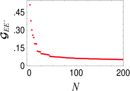
Figure 1: Each dot represents one of the 200 ($N/2$) largest off-diagonal elements $\left|{\cal G}_{EE^{\prime}}\right|$ of the metric. All the diagonal elements are given by ${\cal G}_{EE}=1$.

To illustrate the formalism given above we will take an example in the context of the bound states formed by the scattering of an electron on a positively charged target. This situation is widely employed in atomic physics to study the highly excited (’Rydberg’) states of atoms with a single excited electron. More specifically we will compute the autocorrelation function

$$C(t)=\left\langle\zeta(t=0)\right|\left.\zeta(t)\right\rangle$$ (39)

in two ways: by taking into account the non-Hermitian character of the Hamiltonian on the one hand, and by downright ignoring Hermiticity related issues on the other hand. $\left|C(t)\right|$ is in principle an experimentally observable quantity. If the non-Hermiticity index $\kappa$ is negligible, the two methods of calculation will give nearly identical result (for typical atoms $\kappa$ turns out to be very small, although non-Hermitian issues have always been ignored from first principles).

The long-range Hamiltonian $H_{0}$ in eq (1) contains the radial Hamiltonian of the colliding electron in a centrifugal Coulomb potential as well as the free Hamiltonian of the target (an atomic ion). $f_{i}(\epsilon_{i},r)$ in eq (4) is therefore a Coulomb function regular at the origin (it is also regular at $+\infty$ only if $\epsilon$ belongs to the spectrum of the radial part of $H_{0},$ ie when $\epsilon=-1/2n^{2},$ $n\in{N}$). The radial channel functions $F_{i}(\epsilon_{i},r)$ appearing in eq (14), solutions of the radial part of the redefined $H_{0}$ for $r>r_{0}$, are given by a linear combination of Coulomb functions regular and irregular at the origin, the combination ensuring that $F_{i}(\epsilon_{i},r)$ converges at $\infty$ . For the scattering matrix $K(E)$ we take a $6\times 6$ matrix with a strong energy dependence. We also set the 6 values of $\varepsilon_{i}$ to model the internal energies of the target (we take $\varepsilon_{1}=0$ for the ground state and 5 different values for the excited states of the target). The bound state energies and coefficients are obtained by applying the boundary condition $\left\langle r\right.\left|\psi(E)\right\rangle\rightarrow 0$ as $r\rightarrow\infty$, yielding the system [18]

$$\left[K(E)+R(E)\right]Z(E)=0$$ (40)

where $R(E)$ is a diagonal matrix with elements $R(E)_{ii}=\tan\pi(-2(E-\varepsilon_{i}))^{-1}$. This system is solved numerically for $E$ and then the nontrivial solutions $Z_{i}(E)$ are obtained.  We compute about $N=400$ eigenstates. The radial overlaps (15) are determined analytically, and from there we compute the metric elements $\mathcal{G}_{EE^{\prime}}$. For the overall chunk, the non-Hermiticity index is calculated as $\kappa=0.07$. The ordered distribution of the $N$ largest off-diagonal elements of the metric is shown in Fig. 1.

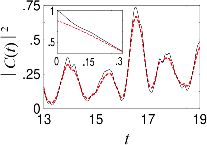
Figure 2: The autocorrelation function $C(t)$ is given as a function of time (in units of the period of the classical orbit of the electron having the mean energy of the initial state). The inset shows the short-time situation. Dashed (colour online: red) curve: the autocorrelation function is computed by ignoring the non-Hermitian character of the problem, following eq (43). Solid line: Result computed by taking non-Hermiticity into account (eq (48)).

We now choose an initial state $\left|\zeta(t=0)\right\rangle$, that we take to be a Gaussian localized radially very far from the target, at the outer turning point of the radial potential for an excited electron (with a mean energy $n=55$), with the target being in its ground state. Initially $\left|\zeta(t=0)\right\rangle$ is defined on an orthogonal basis of $\mathcal{H}_{ph}$ but we assume (and verify numerically) that this state can approximately be expanded on our chunk of computed eigenstates of $\widetilde{H}$ as

$$\left|\zeta(t=0)\right\rangle=\sum a(E)\left|\psi(E)\right\rangle.$$ (41)

where the $a(E)$ are determined by projections. At this point we proceed along the two different lines mentioned above. In the first method of calculation we employ the machinery of standard (Hermitian) quantum mechanics, ignoring non-Hermiticity issues. This may appear absurd in view of the preceding discussion, but this is the way computations are undertaken in applied problems . Moreover this will allow us to assess the relevance of the formalism given above in practical calculations – as we will see by comparing the first method to the second one, where the formalism developed in Sec 3 will be employed.

In the first method the expansions

$$\sum_{E}\left|\psi(E)\right\rangle\left\langle\psi(E)\right|\left[1\textrm{ or }E\textrm{ or }\exp(-iEt/\hbar)\right]$$ (42)

are taken as representations of the unit operator, the Hamiltonian or the evolution operator respectively. The coefficients $a(E)$ of eq (41) are thus given by the projection of this ’unit’ operator as $\left\langle\psi(E)\right|\left.\zeta(t=0)\right\rangle$, and the autocorrelation function (39) follows by employing this ’evolution’ operator,

$$C(t)=\sum_{E}e^{-iEt/\hbar}\left|\left\langle\psi(E)\right|\left.\zeta(t=0)\right\rangle\right|^{2}.$$ (43)

The result is shown in Fig. 2 by the dashed line; in particular the inset shows the short-time evolution, and it may be noticed that at $t=0$ we do not have $C(t=0)=1$, ie $\left|\zeta(t=0)\right\rangle$ is not normalized after the application of the ’unit’ operator (42), which as we know is not the correct unit operator on $\mathcal{H}_{ph}$. Neither is the ’evolution’ defined by eq (42) unitary: $\left\langle\zeta(t)\right|\left.\zeta(t)\right\rangle$ computed with eq (42) shows strong oscillations, displayed in Fig. 3.

The correct method to compute $C(t)$ involves first mapping $\left|\zeta(t=0)\right\rangle$ to $\mathcal{H}$, yielding $\mathcal{G}^{1/2}\left|\zeta(t=0)\right\rangle$ (cf eq (37)), then apply the unitary evolution operator in $\mathcal{H}$ given by eq (31) and finally compute the result with the inner product (36) in $\mathcal{H}$. If we follow the notation (37) and put

$$\left|\phi(t=0)\right\rangle=\mathcal{G}^{1/2}\left|\zeta(t=0)\right\rangle$$ (44)

we get the following equivalent expressions for the autocorrelation function:

$$C(t) = \left(\phi(t=0),\widetilde{U}(t)\phi(t=0)\right)_{\mathcal{G}}$$ (45)

$$= \left\langle\tilde{\phi}(t=0)\right|\widetilde{U}(t)\left|\phi(t=0)\right\rangle$$ (46)

$$= \left\langle\phi(t=0)\right|\mathcal{G}^{-1}\widetilde{U}(t)\left|\phi(t=0)\right\rangle$$ (47)

$$= \left\langle\zeta(t=0)\right|\mathcal{G}^{-1/2}\widetilde{U}(t)\mathcal{G}^{1/2}\left|\zeta(t=0)\right\rangle.$$ (48)

Eqs (45) and (46) give the autocorrelation function as computed entirely in $\mathcal{H}$ whereas eq (48) is the same expression in $\mathcal{H}_{ph}$. $\mathcal{G}^{-1/2}\widetilde{U}(t)\mathcal{G}^{1/2}$ appears as the (correct and unitary) evolution operator in $\mathcal{H}_{ph}$ resulting from the mapping given by eq (34). The computed result is shown by the solid line in Fig. 2, which of course obeys $C(t=0)=1$ (normalization at other times follows from unitarity).

The most salient feature arising from the comparison of the two curves in Fig. 2 concerns the different profiles of the autocorrelation functions. This implies that it will not be possible to recover the correct result (45) from the first method result (43) by simply renormalizing the latter in $\mathcal{H}_{ph}$ (as is sometimes done in practical scattering problems). Conversely it would not make much sense to assume that the initial physical state (41) is known in $\mathcal{H}$, so that one would not need to determine mapping $\mathcal{H}\rightarrow\mathcal{H}_{ph}$. Such an exception happens in the specific but nevertheless important cases in which one is only interested in transitions involving given eigenstates of $\widetilde{H}$.

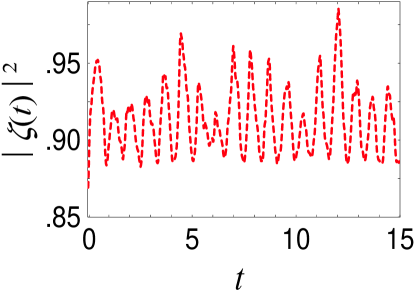
Figure 3: The ’norm’ $\left\langle\zeta(t)\right|\left.\zeta(t)\right\rangle$ is computed as function of time (in units of the period of the mean Kepler orbit). The norm is not conserved because the ’evolution’ operator (42) is Hermitian but not unitary in $\mathcal{H}_{ph}$.

5 Conclusion

We have seen that the widely employed formalism of bound state scattering theory should be properly understood within the framework of non-Hermitian quantum mechanics. Although in typical cases the non-Hermiticity index $\kappa$ is small so that in practice non-Hermitian issues can be ignored, we have given an illustration for which the calculations of experimentally observable quantities require the proper non-Hermitian formulation. The latter has essentially the same structure and tools as the PT-symmetric systems (reformulated in the quasi-Hermitian framework) that are currently being extensively investigated. However in the present case, the physical meaning of non-Hermiticity is more transparent than in the case of PT-symmetric quantum-mechanics. In particular, we have seen that changing the radial interval minutely from $[0,+\infty]$ in the underlying exact problem to $[r_{0},+\infty]$ in the scattering problem leads to an entire redefinition of the Hilbert spaces relevant for quantum mechanics. Indeed, by this change the Hamiltonian $\widetilde{H}$ becomes quasi-Hermitian on $\mathcal{H}_{ph}$. One can then either redefine the inner product, constructing a new Hilbert space $\mathcal{H}$, or map the states and operators to the physical Hilbert space $\mathcal{H}_{ph}$. We have seen that computations are simpler to undertake in $\mathcal{H}$ than in $\mathcal{H}_{ph}$, but except in the specific cases involving the sole eigenstates of the non-Hermitian Hamiltonian, this simplicity is only apparent: as arbitrary physical states are known in $\mathcal{H}_{ph}$, the mapping between the two Hilbert spaces must be explicitly determined anyway, involving the computation of the metric. In the example given in this work the metric was constructed from the numerical calculation of the exact eigenstates of $\widetilde{H}$ in a restricted energy interval of interest.

The interesting insight gained by the existence of an underlying exact Hamiltonian $H^{e}$ is that for scattering states, the physical Hilbert space $\mathcal{H}_{ph}$ is essentially the same as the Hilbert space of the exact problem. But the expansion in $\mathcal{H}_{ph}$ of a physical state in terms of the eigenstates of the exact Hamiltonian differs from the expansion in terms of the eigenstates $\psi(E)$ of the non-Hermitian Hamiltonian (although the physical results – eigenvalues, probability amplitudes – will be identical). Actually the expansion in terms of the eigenstates of the exact Hamiltonian in $\mathcal{H}_{ph}$ is identical to the expansion in terms of the eigenstates of $\widetilde{H}$ in $\mathcal{H}$. These remarks suggest that as far as the scattering eigenstates are concerned, $\mathcal{H}$ is more physical than $\mathcal{H}_{ph}$, where these eigenstates become $\mathcal{G}^{-1/2}\left|\psi(E)\right\rangle$. From a more general standpoint it appears that quantum mechanics requires above all a Hilbert space $\mathcal{H}$ on which the operators are self-adjoint relative to a given inner product, whatever this inner product may be. In this work the Hilbert space $\mathcal{H}_{ph}$ defined with the standard inner product (the $L^{2}$ inner product) only entered the problem because in bound state scattering arbitrary physical states and operators are already known in this space. In general however it is possible to envisage the case in which the standard inner product would not play a special rôle, although such a situation will probably lead to intricate interpretational issues regarding the physical significance of computed quantities.

References

- [1] Bender C M 2005, Contemporary Phys 46 277.
- [2] Bender C M, Brod J, Refig A and Reuter E M 2004 J Phys A 37 10139
- [3] Mostafazadeh A 2003, Preprint arXiv:quant-ph/0310164
- [4] Scholtz F G, Geyer H B and Hahne F J W 1992 Ann Phys 213 74
- [5] Mostafazadeh A and Batal A 2004, J Phys A 37 11645
- [6] Jones H F 2005, J. Phys. A 38 1741
- [7] Mostafazadeh A 2005, J. Phys. A 38 6557
- [8] Bender C M, Chen J H and Milton K A, J. Phys. A 39 1657
- [9] Fano U 1978, Phys Rev A 17 93
- [10] Labastie P and Jalbert G 1992, Phys Rev 46 2581.
- [11] Matzkin A 1999, Phys Rev A 59 2043.
- [12] Newton R G 1982 Scattering theory of waves and particles, NewYork : Springer.
- [13] Fano U and Rau ARP 1986 Atomic Collisions and Spectra, Orlando (USA): Academic Press
- [14] Bloch C 1957, Nucl Phys 4 503
- [15] Kretschmer R and Szymanowski L 2004 Phys. Lett. A 325 112
- [16] Tanaka T 2006, Preprint arXiv:quant-ph/0603075
- [17] Morse P M and Feshbach H 1953, Methods of theoretical physics, New York (USA) : McGraw-Hill.
- [18] Seaton M J 1983, Rep Prog Phys 46, 167