The Quantum Mechanics Problem of the Schrödinger Equation with the Trigonometric Rosen-Morse Potential

C. B. Compean, M. Kirchbach

PACS: 02.30.Gp, 03.65.Ge,12.60.Jv.

1 Introduction

There are few quantum mechanic problems on bound states wave functions that allow for exact solutions. The examples frequented in the standard textbooks on quantum mechanics, mathematical methods, and problem samplers [1] range from the simplest case of the infinite square well potential over the more advanced Harmonic-Oscillator– and Coulomb potentials and culminate with the more sophisticated Morse–, Eckart–, the trigonometric Scarf and the hyperbolic Rosen-Morse potentials, which have importance in atomic and molecular spectroscopy. All the known exactly soluble potentials are attached to observed physical spectra and the corresponding wave functions are expressed in terms of the well known classical orthogonal polynomials [2].

Within the context of supersymmetric quantum mechanics, one encounters two more potentials, the hyperbolic Scarf and the trigonometric Rosen-Morse potentials, that are claimed to allow for exact solutions however in terms of Jacobi polynomials with complex arguments and complex indices [3], [4] a less appealing feature indeed given the observation on the non-trivial orthogonality properties of the complex Jacobi polynomials as reported in the current mathematical literature [5], [6].

In our previous work [7] we demonstrated within the context of supersymmetric quantum mechanics that the one-dimensional Schrödinger equation with the trigonometric Rosen-Morse potential is exactly soluble in terms of real orthogonal polynomials of a new type. Here we work out these solutions anew within the different context of interpolation between the Coulomb and the infinite square well potentials and hint on the possible importance of the trigonometric Rosen-Morse potential for QCD.

The paper is organized as follows. In the next section we analyze the shape of the trigonometric Rosen-Morse potential. In section III we present the exact real orthogonal polynomial solutions of the corresponding Schrödinger equation. The paper ends with a brief concluding section.

2 The shape of the trigonometric Rosen-Morse potential

We adopt the following form of the trigonometric Rosen-Morse potential [3],[4]

$$v(z)=-2b\cot z+a(a+1)\csc^{2}z\,,$$ (1)

with $a>-1/2$ and displayed in Fig. 1. Here,

$$z=\frac{y}{d}, v(z)=V(zd)/(\hbar^{2}/2md^{2}),$$

$$\epsilon_{n} = E_{n}/(\hbar^{2}/2md^{2})\,,$$ (2)

with $y$ being the one-dimensional variable, $d$ a properly chosen length scale, $V(y)$ the potential in ordinary coordinate space, and $E_{n}$ the energy level.

Our point here is that $v(z)$ interpolates between the Coulomb and the infinite wall potential going through an intermediary region of linear $z$ and harmonic-oscillator $z^{2}$ dependences. To see this (besides inspection of Fig. 1) it is quite instructive to expand the potential in a Taylor series which for appropriately small $z$, takes the form of a Coulomb-like potential with a centrifugal-barrier like term provided by the $\csc^{2}z$ part,

$$v(z)\approx-\frac{2b}{z}+\frac{a(a+1)}{z^{2}}\,.$$ (3)

In an intermediary range where inverse powers of $z$ may be neglected, one finds the linear plus a harmonic-oscillator potentials

$$v(z)\approx\frac{2b}{3}\,z+\frac{a(a+1)}{36}z^{2}\,.$$ (4)

Finally, as long as $\cot\,z\stackrel{{\scriptstyle z\to\pi}}{{\longrightarrow}}\infty$ and $\csc^{2}\,z\stackrel{{\scriptstyle z\to\pi}}{{\longrightarrow}}\infty$, the potential obviously evolves to an infinite wall. Below we shall show that in the parameter limit $a\to 0$ and $b\to 0$, the wave functions recover those of the infinite square wall.

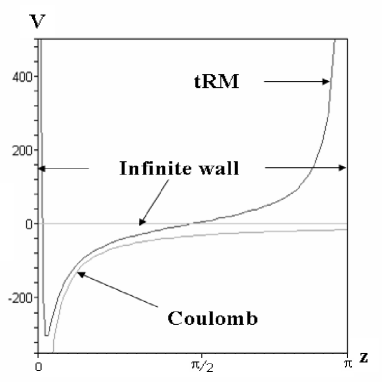
Figure 1: The trigonometric Rosen-Morse potential and its proximity to the Coulomb-like and the infinite square wall potentials for $a=0.25$ and $b=1$.

Above shape captures surprisingly well the essentials of the QCD quark-gluon dynamics where the one gluon exchange gives rise to an effective Coulomb-like potential, while the self-gluon interactions produce a linear potential as established by lattice calculations of hadron properties. Finally, the infinite wall piece of the trigonometric Rosen-Morse potential provides the regime suited for asymptotically free quarks.

By above considerations one is tempted to conclude that the potential under consideration may be a good candidate for an effective QCD potential.

3 Exact spectrum and wave functions of the trigonometric Rosen-Morse potential

The one-dimensional Schrödinger equation with the trigonometric Rosen-Morse potential (tRM) reads:

$${d^{\,2}\ R_{m}(z)\over d\ z^{2}}+\left(2b\cot z-a(a+1)\csc^{2}z+\epsilon\right)R_{m}(z)=0\,,$$ (5)

Our pursued strategy in solving it will be to first reshape it to the particular case of a self-adjoined Sturm-Liouville equation of the form

$$s(x){{d^{\,2}F_{m}(x)}\over{d\ x^{2}}}+{1\over{w(x)}}\left({{d\ s(x)w(x)}\over{d\ x}}\right){d\ F_{m}(x)\over d\ x}+\lambda_{m}\ F_{m}(x)=0\ ,$$ (6)

and then try to solve it by means of the so called Rodrigues representation

$$F_{m}(x)=\frac{1}{K_{m}w(x)}{d^{m}\over d\ x^{m}}(w(x)\ s(x)^{m})\ ,$$ (7)

where $K_{m}$ is the normalization constant of the $F_{m}(x)$ polynomials. The constant $\lambda_{m}$ in Eq. (6) is supposed to satisfy the following condition [8]

$$\lambda_{m} = -m\left(K_{1}{{d\ F_{1}(x)}\over{d\ x}}+{1\over 2}(m-1){{d^{\,2}s(x)}\over{d\ x^{2}}}\right)\,,\quad\mbox{with}$$

$$F_{1}(x) = {1\over{K_{1}w(x)}}\left({{d\ s(x)w(x)}\over{d\ x}}\right)\,.$$ (8)

Sturm-Liouville equations of the type given in Eq. (6) are called hypergeometric equations.

The chosen strategy is inspired by the observation that all the classical polynomials have been obtained precisely from those very Eqs. (6)–(8), appear orthogonal with respect to the weight function $w(x)$ and obey the following restrictions (see Chpt. 10 in Ref. [8] for more details): (i) $F_{1}(x)$ is a polynomial of first order, (ii) $s(x)$ is a polynomial of at most second order and real roots, (iii) $w(x)$ is real, positive and integrable within a given interval $[a,b]$, and satisfies the boundary conditions

$$w(a)s(a)=w(b)s(b)=0\ .$$ (9)

We here draw attention to the fact that the exact solutions of Eq. (5) can be expressed in terms of real orthogonal polynomials that solve a hypergeometric differential equation of a new class.

Back to Eq. (5) we factorize the wave function as

$$R_{m}(z)=\textrm{ e}^{-\alpha z/2}(1+\cot^{2}z)^{\frac{-(1-\beta)}{2}}C^{(\alpha,\beta)}_{m}(\cot z)\,,$$ (10)

with $\alpha$ and $\beta$ being constants. Upon introducing the new variable $x=\cot z$ and substituting the above factorization ansatz into Eq. (10) and a subsequent division by $(1+x^{2})^{(1-\beta)/2}$ one finds the equation

$$(1+x^{2})\frac{d^{\,2}\ C^{(\beta,\alpha)}_{m}(x)}{d\ x^{2}}+2\left({\alpha\over 2}+\beta x\right){d\ C^{(\beta,\alpha)}_{m}(x)\over d\ x}$$ (11)

$$+ \left((-\beta(1-\beta)-a(a+1))+{(-\alpha(1-\beta)+2b)x+\left(\left({\alpha\over 2}\right)^{2}-(1-\beta)^{2}+\epsilon_{n}\right)\over 1+x^{2}}\right)C^{(\beta,\alpha)}_{m}(x)=0\ ,$$

which is suited for comparison with the hypergeometric equation (6).

The derivative terms in Eq. (11) have already the desired form of Eq. (6). As a first observation one encounters $s(x)$ as

$$s(x)=1+x^{2}\,,$$ (12)

and of purely imaginary roots. Nonetheless, as we shall see immediately, this is not to turn out to be a great obstacle on the way of finding the exact real solutions of Eq. (10). Next, the function that plays the role of the weight-function is

$$w^{(\beta,\alpha)}(x)=(1+x^{2})^{\beta-1}e^{-\alpha\cot^{-1}x}\,.$$ (13)

These $s(x)$ and $w^{(\beta,\alpha)}(x)$ functions allow to write the following new hypergeometric differential equation for the polynomials $C_{m}^{(\beta,\alpha)}(x)$:

$$(1+x^{2})\frac{d^{\,2}\ C^{(\beta,\alpha)}_{m}(x)}{d\ x^{2}}+2\left({\alpha\over 2}+\beta x\right){d\ C^{(\beta,\alpha)}_{m}(x)\over d\ x}\ -m(2\beta+m-1)C_{m}^{(\beta,\alpha)}(x)=0\,.$$ (14)

Equation (14) generalizes the hypergeometric equation and represents a new equation in mathematical physics that is important on its own.

As in the case of the Jacobi polynomials, also the weight function giving rise to Eq. (14) happens to be parameter dependent. If the potential equation (11) is to coincide with the polynomial equation (14) then the coefficient in front of the $1/(x^{2}+1)$ term in (11) has to nullify. This imposes the following conditions on the indices of the polynomials which are to enter the Schrödinger wave function:

$$-\alpha(1-\beta)+2b=0\ ,$$ (15)

$$\left({\alpha\over 2}\right)^{2}-(1-\beta)^{2}+\epsilon=0\,.$$ (16)

With that the Eq. (11) to which one has reduced the original Schrödinger equation amounts to

$$(1+x^{2}){d^{\,2}\ C_{m}^{(\beta,\alpha)}(x)\over d\ x^{2}}+2\left({\alpha\over 2}+\beta x\right){d\ C_{m}^{(\beta,\alpha)}(x)\over d\ x}+(-\beta(1-\beta)-a(a+1))C_{m}^{(\beta,\alpha)}(x)=0\ .$$ (17)

The final step is to identify the constant term in the latter equation with the one in Eq. (14) which leads to a third condition

$$-\beta(1-\beta)-a(a+1)=-m(2\beta+m-1)\ .$$ (18)

Remarkably, Eqs. (15), (16) and (18) indeed allow for consistent solutions for $\alpha$, $\beta$, and $\epsilon$ and given by (upon renaming $m$ by $(n-1))$:

$$\beta_{n}=-(n+a)+1\ , \alpha_{n}={2b\over n+a}\ ,$$

$$\epsilon_{n} = (n+a)^{2}-{b^{2}\over(n+a)^{2}}\ ,$$ (19)

with $n\geq 1$. In this way Eq. (19) provides the exact tRM spectrum displayed in Fig. 2.

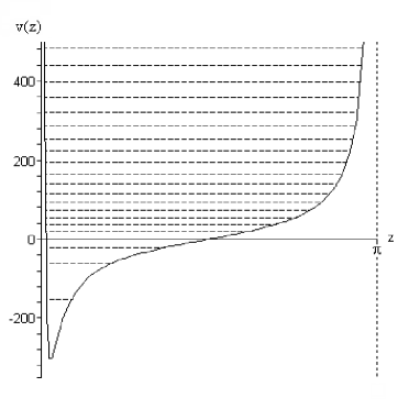
Figure 2: Energy levels within the trigonometric Rosen-Morse potential for $a=0.25$ and $b=1$.

With that all the necessary ingredients for the solution of Eq. (17) have been prepared. In now exploiting the Rodrigues representation (when making the $n$ dependence explicit)

$$C^{(\beta_{n},\alpha_{n})}_{n}(x)={1\over K_{n}\ w^{(\beta_{n},\alpha_{n})}(x)}{d^{n-1}\over d\ x^{n-1}}\left(w^{(\beta_{n},\alpha_{n})}(x)\ s(x)^{n-1}\right)\,,$$ (20)

allows for the systematic construction of the solutions of Eq. (17). To be specific, the lowest five $C_{n}^{(\beta_{n},\alpha_{n})}(x)$ polynomials that enter the exact wave function of the Schrödinger equation with the trigonometric Rosen-Morse potential are now obtained as:

$$C^{(\beta_{1},\alpha_{1})}_{1}(x) = {1\over K_{1}}\ ,$$ (21)

$$C^{(\beta_{2},\alpha_{2})}_{2}(x) = {2\over K_{2}}\left(-(1+a)x+{b\over 2+a}\right)\ ,$$ (22)

$$C^{(\beta_{3},\alpha_{3})}_{3}(x) = {2\over K_{3}}\left((1+a)(2a+3)x^{2}-2(2a+3){b\over 3+a}x+\left({2b^{2}\over(3+a)^{2}}-(1+a)\right)\right)\ ,$$ (23)

$$C^{(\beta_{4},\alpha_{4})}_{4}(x) = {4\over K_{4}}\left(-(1+a)(2a+3)(2+a)x^{3}+3(a+2)(2a+3){b\over(4+a)}x^{2}\right.$$ (24)

$$\left.-3(2+a)\left(2{b^{2}\over(4+a)^{2}}-(1+a)\right)x+\left({2b^{3}\over(4+a)^{3}}-(3a+4){b\over 4+a}\right)\right)\ ,$$

$$C^{(\beta_{5},\alpha_{5})}_{5}(x) = {4\over K_{5}}\left((1+a)(2a+3)(2+a)(2a+5)x^{4}-4(2a+3)(2+a)(2a+5){b\over(5+a)}x^{3}\right.$$ (25)

$$\left.+6(2+a)(2a+5)\left({2b^{2}\over(5+a)^{2}}-(1+a)\right)x^{2}\right.$$

$$-4(2a+5)\left({2b^{3}\over(5+a)^{3}}-(3a+4){b\over 5+a}\right)x$$

$$\left.+\left({4b^{4}\over(5+a)^{4}}-{4b^{2}\over(5+a)^{2}}(3a+5)+3(2+a)(1+a)\right)\right)\ ,$$

where $x=\cot z$.
Above polynomials solve exactly Eq. (17) which can be immediately cross-checked by back-substituting Eqs. (25) into Eq. (17). Employing symbolic mathematical programs is quite useful in that regard.

Notice that in terms of $w^{(\beta_{n},\alpha_{n})}(x)$ the wave function is expressed as

$$R_{n}(\cot^{-1}x)=\sqrt{w^{(\beta_{n},\alpha_{n})}(x)}C_{n}^{(\beta_{n},\alpha_{n})}(x)\,.$$ (26)

In Figs. 3 we display as an illustrative example the wave functions for the first four (unnormalized) levels. A version interesting for physical application (see concluding Section) is the one with $a=0$ when the potential becomes

$$v(z)=-2b\cot\,z\,,$$ (27)

and in which case the normalization constant can be calculated in the following closed form:

$$K_{n}=\left({(n!)^{2}n^{3}(1-\textrm{ e}^{-2\pi b/n})\over 4b(b^{2}+n^{4})}\right)^{1/2}\ .$$ (28)

The associated energy spectrum is given by

$$\epsilon_{n}=n^{2}-\frac{b^{2}}{n^{2}}\,.$$ (29)

Correspondingly, the wave functions simplify to

$$R_{n}(z)=e^{-\frac{bz}{n}}\sin^{n}zC_{n}^{(-n+1,\alpha_{n})}(\cot\,z)\,.$$ (30)

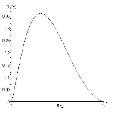
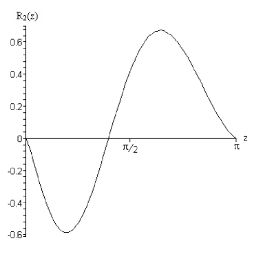
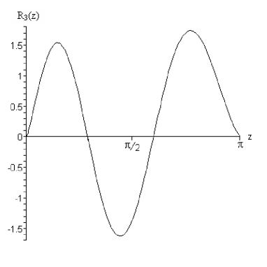
(a) (b) (c) (d)

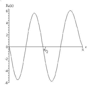
Figure 3: Wave functions for the first four levels in the trigonometric Rosen-Morse potential for $a=$0.25 and $b=$1.

Next one can check orthogonality of the physical solutions and obtain it as it should be as

$$\int_{0}^{\pi}dz\ R_{n}(z)R_{n^{\prime}}(z)=\delta_{n\ n^{\prime}}\,.$$ (31)

The orthogonality of the wave functions $R_{n}(z)$ implies in $x$ space orthogonality of the $C_{n}^{(\beta_{n},\alpha_{n})}(x)$ polynomials with respect to $w^{(\beta_{n},\alpha_{n})}(x)\frac{dz}{dx}$ due to the variable change. As long as $\frac{d\cot^{-1}z}{dx}=-1/(1+x^{2})\equiv-1/s(x)$ then the orthogonality integral takes the form

$$\int_{-\infty}^{\infty}{dx\over s(x)}\sqrt{w^{(\beta_{n},\alpha_{n})}(x)}C_{n}^{(\beta_{n},\alpha_{n})}(x)\sqrt{w^{(\beta_{n^{\prime}},\alpha_{n^{\prime}})}(x)}C_{n^{\prime}}^{(\beta_{n^{\prime}},\alpha_{n^{\prime}})}(x)=\delta_{n\ n^{\prime}}\ .$$ (32)

As long as the new polynomials $C_{n}^{(\beta,\alpha)}(x)$ satisfy a new hypergeometric equation that generalizes the Jacobi equation from $s(x)=(1-x^{2})$ to $s(x)=(1+x^{2})$ we shall refer to the new polynomials as generalized classical polynomials. Equations (31) and (32) show that the new solutions have well defined orthogonality properties on the real axes, which qualifies them as comfortable wave functions in quantum mechanics applications. It is perhaps quite instructive to compare Eq. (14) to the Jacobi equation

$$(1-x^{2})\frac{d^{2}P_{n}^{(\gamma,\delta)}(x)}{dx^{2}}+(\gamma-\delta-(\gamma+\delta+2)x)\frac{dP_{n}^{(\gamma,\delta)}(x)}{dx}-m(m+\gamma+\delta+1)P_{n}^{(\gamma,\delta)}(x)=0\,.$$ (33)

Upon complexification of the argument, $x\to ix$, the latter equation transforms into

$$(1+x^{2})\frac{d^{2}P_{n}^{(\gamma,\delta)}(ix)}{dx^{2}}+i(\gamma-\delta-i(\gamma+\delta+2)x)\frac{dP_{n}^{(\gamma,\delta)}(ix)}{dx}+m(m+\gamma+\delta+1)P_{n}^{(\gamma,\delta)}(ix)=0\,.$$ (34)

From a formal point of view, Eq. (34) can be made to coincide with Eq. (14) for the following parameters:

$$\gamma=\beta-1-\frac{i\alpha}{2}\,,\quad\delta=\beta-1+\frac{i\alpha}{2}\,.$$ (35)

In this sense one relates in the literature the Jacobi polynomials of complex arguments and indices to the solutions of the trigonometric Rosen-Morse potential. This relation is in our opinion a bit misleading because the real orthogonal $C_{n}^{(\beta,\alpha)}(x)$ polynomials are apparently a specie that is fundamentally different from $P_{n}^{\left(\beta-1-\frac{i\alpha}{2},\beta-1+\frac{i\alpha}{2}\right)}(ix)$.

4 Discussion and concluding remarks

The physically interesting case of the potential considered here is the one of a vanishing $a$ parameter and the spectrum given in Eq. (29). It fits perfectly well the mass splittings of the nucleon and $\Delta$ resonances, results due to Refs. [9],[7]. This finding seems to provide a further hint on the possible relevance of the trigonometric Rosen-Morse potential as an effective QCD confinement potential that should not be ignored.

Moreover, the exact wave functions of this potential reveal quite instructive asymptotic behaviors. In the zero parameter limit, $a\to 0$, and $b\to 0$, it is easy to show by explicit calculation that the $R_{n}(z)$ recover the wave functions of the infinite square wall potential,

$$\lim_{a\to 0,b\to 0}\,R_{n}(z)=\lim_{a\to 0,b\to 0}\exp{(-bz)}\sin^{n+a}C_{n}^{(\beta_{n},\alpha_{n})}(\cot z)=(-1)^{n-1}\sqrt{\frac{2}{\pi}}\sin nz\,,$$ (36)

which describe “free” particle motion within a confining potential. In that regard one may think of the asymptotically free quarks.

The other instructive asymptotic limit is the one of small $r$ with $r$ associated with the relative distance between two particles within the three dimensional version of the potential in which case Eq. (5) would refer to the radial part, $U_{n}(r)=R_{n}(r)/r$, of the wave function and zero angular momentum. In this case, from Eq. (26) one reads off the ground state wave function as

$$U_{1}(r)=\frac{R_{1}(r)}{r}=\exp{\left(-\frac{\alpha_{1}r}{2}\right)}\frac{\sin^{1+a}r}{r}C^{(a,\alpha_{1})}_{1}(\cot r)\,.$$ (37)

For small $r$ and $a=0$ the latter expression approaches the ground state of the hydrogen atom, $\exp{\left(-\frac{\alpha_{1}r}{2}\right)}$, which would be the nucleon wave function as well if one could ignore the multi-gluon self interactions and approximate the three quark problem by a two body quark-diquark one. This is certainly quite a rough and unrealistic limiting case which nonetheless reveals the correct long range one-gluon exchange mechanism of QCD as part of the physical content of the tRM potential.

All in all, the Schrödinger equation with the trigonometric Rosen-Morse potential, besides being an interesting quantum mechanics exercise and besides leading to a new differential equation of mathematical physics that is important in its own, seems to bear a rich information on the quark-gluon dynamics that may qualify it as an effective QCD potential, a possibility that should be kept in mind for future research.

References

-
[1]
J. J. Sakurai, Modern Quantum Mechanics
(Addison-Wesley Pub. Co., Reading 1994);
G. B. Arfken, H. J. Weber, Mathematical Methods for Physicists, 6th ed. (Elsevier-Academic Press, Amsterdam, 2005);
I. V. Kogan, Problems in Quantum Mechanics (Prentice-Hall, Engelwood, 1963);
S. Flügge, Practical Quantum Mechanics (Springer, New York, 1974). - [2] M. Abramowitz, I. A. Stegun, Handbook of Mathematical Functions with Formulas, Graphs and Mathematical Tables, Dover, 2nd edition, New York, 1972).
-
[3]
C. V. Sukumar, J. Phys. A:Math. Gen. 18, 2917 (1998);
C. V. Sukumar, AIP proceedings 744, eds. R. Bijker et al., Supersymmetries in physics and applications, (New York, 2005), p. 167. - [4] F. Cooper, A. Khare, U. P. Sukhatme, Supersymmetry in Quantum Mechanics (World Scientific, Singapore, 2001).
- [5] A. B. J. Kuijlaars, A. Martinez-Finkelshtein, R. Orive, Orthogonality of Jacobi Polynomials with General Parameters, E-Print ArXiv: math.CA/0301037 (2003).
- [6] B. Beckermann, J. Coussement, W. Van Asshe, Multiple Wilson and Jacobi-Piñeiro Polynomials, E-Print ArXiv: math.CA/0311055 (2003).
- [7] C. B. Compean, M. Kirchbach, J. Phys. A:Math.Gen. 39, 547 (2006).
- [8] Phylippe Dennery, André Krzywicki, Mathematics for Physicists (Dover, New York, 1996).
- [9] M. Kirchbach, M. Moshinsky, Yu. F. Smirnov, Phys. Rev. D 64, 114005 (2001).