Spin entanglement loss by local correlation transfer to the momentum

Abstract

We show the decrease of spin-spin entanglement between two $s=\frac{1}{2}$ fermions or two photons due to local transfer of correlations from the spin to the momentum degree of freedom of one of the two particles. We explicitly show how this phenomenon operates in the case where one of the two fermions (photons) passes through a local homogeneous magnetic field (optically-active medium), losing its spin correlations with the other particle.

I INTRODUCTION

Bipartite and multipartite entanglement is considered a basic resource in most applications of quantum information, communication, and technology  (see for instance Refs. Nielsen and Chuang (2000); Galindo and Martín-Delgado (2002)). Entanglement is fragile, and it is well-known that in some cases interactions with an environment external to the entangled systems may decrease the quantum correlations, degrading this valuable resource Yu and Eberly (2002, 2003, 2004); Dodd and Halliwell (2004); Nikolić and Souma (2005); Carvalho et al. (2005); França Santos et al. et al. (2005). Momentum acts as a very special environment which every particle possesses and cannot get rid of. Consider for instance a bipartite system which initially is spin-entangled and with the momentum distributions factorized. It will decrease its spin-spin correlations provided any of the two particles entangles its spin with its momentum. This simple idea was studied in the natural framework of special relativity, where changing the reference frame induces Wigner rotations that entangle each spin with its momentum Peres et al. (2002); Czachor (2005); Alsing and Milburn (2002); Gingrich and Adami (2002); Pachos and Solano (2003); Czachor and Wilczewski (2003); Gingrich et al. (2003); Lamata et al. (2005). However, this is just a kinematical, frame-dependent effect only, and not a real dynamical interaction. On the other hand, this type of reasoning is also related to which-path detection Scully et al. (2005). In addition, an experiment observing photon polarization disentanglement by correlation transfer, in this case to the photon’s position, was performed França Santos et al. (2005). Can local interactions entangling spin with momentum produce the loss of non-local spin-spin entanglement? To our knowledge this question has not been explored in the literature. More remarkably, any particle owns a certain momentum distribution acting as an intrinsic environment, which can never be eliminated by improving the experimental conditions. But how does this fact affect the spin-spin correlations? This is the question we want to analyze in this paper.

In Sec. II we consider a bipartite system, composed by two $s=\frac{1}{2}$ fermions or two photons, which are initially in a Bell spin state $|\Psi^{-}\rangle$. We use a formalism Lamata et al. (2005) that shows the decrease of spin entanglement whenever an interaction locally entangling spin with momentum takes place. We obtain the negativity $N$ Vidal and Werner (2002) in terms of an integral depending on the spin rotation angle conditional to the momentum. In Sec. III we analyze this physical phenomenon in two specific situations: (i) Two spin-$\frac{1}{2}$ fermions in a $|\Psi^{-}\rangle$ Bell state, with Gaussian momentum distributions, that fly apart while one of them passes through a local magnetic field. Their spin entanglement decreases as a consequence of the transfer of correlations to the momentum of the latter fermion. And (ii) Two photons in a polarization $|\Psi^{-}\rangle$ Bell state, with Gaussian momentum distributions, which separate while one of them traverses an optically-active medium. This medium will entangle the polarization with the momentum and thus decrease the polarization entanglement. This is an unavoidable source of decoherence. In Sec. IV we show that the apparent purely quantum communication resulting from these procedures is not possible. Classical communication has to be exchanged for the protocol to operate. The paper ends with our conclusions in Sec. V.

II SPIN ENTANGLEMENT LOSS BY CORRELATION TRANSFER TO THE MOMENTUM

We consider a maximally spin-entangled state for two $s=\frac{1}{2}$ fermions $A$ and $B$, or two photons $A$ and $B$. The case we analyze is that in which the two particles are far apart already. This avoids dealing with symmetrization issues. Indeed, our state is the maximally entangled one for two $s=\frac{1}{2}$ spins or polarizations, containing 1 ebit.

$$|\Psi^{-}_{{\bf{p}}}\rangle\!\!\! := \!\!\!\frac{1}{\sqrt{2}}[\Psi_{\uparrow}^{(\rm a)}({\bf{p_{a}}})\Psi_{\downarrow}^{(\rm b)}({\bf{p_{b}}})-\Psi_{\downarrow}^{(\rm a)}({\bf{p_{a}}})\Psi_{\uparrow}^{(\rm b)}({\bf{p_{b}}})],$$

where ${\bf{p_{a}}}$ and ${\bf{p_{b}}}$ are the corresponding momentum vectors of particles $A$ and $B$, and

$$\Psi_{\uparrow}({\bf{p}}) := {\cal M}({\bf{p}})|\!\!\uparrow\rangle=\left(\begin{array}[]{cccc}{\cal M}({\bf{p}})\\ 0\\ \end{array}\right),$$ (4)

$$\Psi_{\downarrow}({\bf{p}}) := {\cal M}({\bf{p}})|\!\!\downarrow\rangle=\left(\begin{array}[]{cccc}0\\ {\cal M}({\bf{p}})\\ \end{array}\right),$$ (7)

with bimodal momentum distribution ${\cal M}({\bf{p}}):=\frac{1}{\sqrt{2}}(\delta_{{\bf{p}}{\bf{p_{1}}}}+\delta_{{\bf{p}}{\bf{p_{2}}}})$. ${\bf{p}}_{1}$ and ${\bf{p}}_{2}$ are the two momentum values considered associated to particle $A$, ${\bf{p}}_{1}^{(\rm a)}$, ${\bf{p}}_{2}^{(\rm a)}$, on the one hand, and particle $B$, ${\bf{p}}_{1}^{(\rm b)}$, ${\bf{p}}_{2}^{(\rm b)}$, on the other hand. We consider for the time being this kind of distribution for illustrative purposes. At the end of this section we generalize our results to arbitrary momentum distributions of the two particles. $|\!\!\uparrow\rangle$ and $|\!\!\downarrow\rangle$ represent either spin vectors pointing up and down along the $z$-axis, in the fermionic case, or right-handed and left-handed circular polarizations, in the photonic case. If we trace out the momentum degrees of freedom in Eq. (LABEL:deco1), we obtain the usual spin Bell state, $|\Psi^{-}\rangle$.

We consider a local interaction which entangles the spin of each particle with its momentum through a real unitary (orthogonal) transformation $U$. We choose a real transformation for the sake of simplicity and in order to obtain fully analytical results. The generalization for inclusion of complex phases is straightforward but adds nothing of relevance in this section. We will take it fully into account in Sec. III.

Each state vector in Eq. (7) transforms as

$$\Psi_{\uparrow}({\bf{p}})=\left(\begin{array}[]{cccc}{\cal M}({\bf{p}})\\ 0\\ \end{array}\right)\rightarrow$$ (10)

$$U[\Psi_{\uparrow}({\bf{p}})]=\left(\begin{array}[]{cccc}\cos\theta_{{\bf{p_{1}}}}\\ \sin\theta_{{\bf{p_{1}}}}\\ \end{array}\right)\frac{\delta_{{\bf{p}}{\bf{p_{1}}}}}{\sqrt{2}}+\left(\begin{array}[]{cccc}\cos\theta_{{\bf{p_{2}}}}\\ \sin\theta_{{\bf{p_{2}}}}\\ \end{array}\right)\frac{\delta_{{\bf{p}}{\bf{p_{2}}}}}{\sqrt{2}},$$ (15)

$$\Psi_{\downarrow}({\bf{p}})=\left(\begin{array}[]{cccc}0\\ {\cal M}({\bf{p}})\\ \end{array}\right)\rightarrow$$ (18)

$$U[\Psi_{\downarrow}({\bf{p}})]=\left(\begin{array}[]{cccc}-\sin\theta_{{\bf{p_{1}}}}\\ \,\,\,\,\,\cos\theta_{{\bf{p_{1}}}}\\ \end{array}\right)\frac{\delta_{{\bf{p}}{\bf{p_{1}}}}}{\sqrt{2}}+\left(\begin{array}[]{cccc}-\sin\theta_{{\bf{p_{2}}}}\\ \,\,\,\,\,\cos\theta_{{\bf{p_{2}}}}\\ \end{array}\right)\frac{\delta_{{\bf{p}}{\bf{p_{2}}}}}{\sqrt{2}},$$ (23)

(24)

where $\theta_{{\bf{p_{1}}}}$ and $\theta_{{\bf{p_{2}}}}$ produce a spin-momentum entangled state whenever $\theta_{{\bf{p_{1}}}}\neq\theta_{{\bf{p_{2}}}}$. The effect of this local interaction is that a part of the non-local spin-spin entanglement is transferred to the spin-momentum one, and the degree of entanglement of the spins decreases. To show this, we consider the state (LABEL:deco1) evolved with the transformation $U$, and trace out the momenta.

$$\mathrm{Tr}_{\rm{\bf{p_{a}}},{\bf{p_{b}}}} (U|\Psi^{-}_{{\bf{p}}}\rangle\langle\Psi^{-}_{{\bf{p}}}|U^{{\dagger}})$$ (25)

$$= \frac{1}{2}\;\sum_{s,s^{\prime}}ss^{\prime}\mathrm{Tr}_{\rm{\bf{p_{a}}}}(U^{(\rm a)}[\Psi^{(\rm a)}_{s}({\bf{p_{a}}})]\{U^{(\rm a)}[\Psi^{(\rm a)}_{s^{\prime}}({\bf{p_{a}}})]\}^{{\dagger}})$$

$$\otimes\mathrm{Tr}_{\rm{\bf{p_{b}}}}(U^{(\rm b)}[\Psi^{(\rm b)}_{-s}({\bf{p_{b}}})]\{U^{(\rm b)}[\Psi^{(\rm b)}_{-s^{\prime}}({\bf{p_{b}}})]\}^{{\dagger}}),$$

where $ss^{\prime}:=\delta_{s,s^{\prime}}-\delta_{s,-s^{\prime}}$. It can be appreciated in Eq. (25) that the expression is decomposable in sum of tensor products of 2$\times$2 spin blocks, each corresponding to each particle. We compute now the different blocks, corresponding to the four possible tensor products of the states (24)

$$\mathrm{Tr}_{\rm{\bf{p}}}[U\Psi_{\uparrow}(U\Psi_{\uparrow})^{{\dagger}}] = \frac{1}{2}\left(\begin{array}[]{cc}c_{1}^{2}+c_{2}^{2}&c_{1}s_{1}+c_{2}s_{2}\\ c_{1}s_{1}+c_{2}s_{2}&s_{1}^{2}+s_{2}^{2}\end{array}\right),$$ (28)

$$\mathrm{Tr}_{\rm{\bf{p}}}[U\Psi_{\uparrow}(U\Psi_{\downarrow})^{{\dagger}}] = \frac{1}{2}\left(\begin{array}[]{cc}-c_{1}s_{1}-c_{2}s_{2}&c_{1}^{2}+c_{2}^{2}\\ -s_{1}^{2}-s_{2}^{2}&c_{1}s_{1}+c_{2}s_{2}\end{array}\right),$$ (31)

$$\mathrm{Tr}_{\rm{\bf{p}}}[U\Psi_{\downarrow}(U\Psi_{\uparrow})^{{\dagger}}] = \frac{1}{2}\left(\begin{array}[]{cc}-c_{1}s_{1}-c_{2}s_{2}&-s_{1}^{2}-s_{2}^{2}\\ c_{1}^{2}+c_{2}^{2}&c_{1}s_{1}+c_{2}s_{2}\end{array}\right),$$ (34)

$$\mathrm{Tr}_{\rm{\bf{p}}}[U\Psi_{\downarrow}(U\Psi_{\downarrow})^{{\dagger}}] = \frac{1}{2}\left(\begin{array}[]{cc}s_{1}^{2}+s_{2}^{2}&-c_{1}s_{1}-c_{2}s_{2}\\ -c_{1}s_{1}-c_{2}s_{2}&c_{1}^{2}+c_{2}^{2}\end{array}\right),$$ (37)

where $c_{i}:=\cos(\theta_{{\bf{p_{i}}}})$ and $s_{i}:=\sin(\theta_{{\bf{p_{i}}}})$. This way, it is possible to compute the effects of the local interaction $U$ in the state $|\Psi^{-}_{{\bf{p}}}\rangle$ after tracing out the momentum. We choose equal interaction angles for the two particles, $\theta_{{\bf{p_{i}}}}^{(\rm a)}=\theta_{{\bf{p_{i}}}}^{(\rm b)}$, as a natural simplification. The resulting bipartite spin state is

$$\left(\!\!\!\begin{array}[]{cccc}\frac{1}{4}s_{12}^{2}&0&0&\frac{1}{4}s_{12}^{2}\\ 0&\frac{1}{4}(1+c_{12}^{2})&-\frac{1}{4}(1+c_{12}^{2})&0\\ 0&-\frac{1}{4}(1+c_{12}^{2})&\frac{1}{4}(1+c_{12}^{2})&0\\ \frac{1}{4}s_{12}^{2}&0&0&\frac{1}{4}s_{12}^{2}\\ \end{array}\!\!\!\right),\\$$ (38)

where $s_{12}:=\sin(\theta_{{\bf{p_{1}}}}-\theta_{{\bf{p_{2}}}})$ and $c_{12}:=\cos(\theta_{{\bf{p_{1}}}}-\theta_{{\bf{p_{2}}}})$. The entanglement monotone we will use is the negativity Vidal and Werner (2002), defined as $N:=\max\{0,-2\lambda_{\rm min}\}$, where $\lambda_{\rm min}$ is the smallest eigenvalue of the partial transpose (PT) matrix of Eq. (38). It is very easily computable, and is found to be

$$N=\cos^{2}(\theta_{{\bf{p_{1}}}}-\theta_{{\bf{p_{2}}}}).$$ (39)

From this expression it can be appreciated that for $\theta_{{\bf{p_{1}}}}=\theta_{{\bf{p_{2}}}}$ the entanglement remains maximal (1 ebit), and for $\theta_{{\bf{p_{1}}}}$ separating from $\theta_{{\bf{p_{2}}}}$ the entanglement decreases, until $\theta_{{\bf{p_{1}}}}-\theta_{{\bf{p_{2}}}}=\pi/2$, where it vanishes and the state becomes separable. We plot this behavior in Figure 1, showing the negativity $N$ in Eq. (39) as a function of $\theta_{{\bf{p_{1}}}}$ and $\theta_{{\bf{p_{2}}}}$. Every local interaction producing spin-momentum entanglement will in general diminish the initial maximal spin-spin entanglement of the two particles, thus degrading this resource. This result is valid either for $s=\frac{1}{2}$ fermions or photons, as they both have a two-dimensional internal Hilbert space.

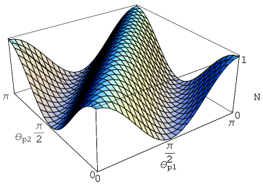
Figure 1: (Color online) Negativity $N$ in Eq. (39) as a function of $\theta_{{\bf{p_{1}}}}$ and $\theta_{{\bf{p_{2}}}}$.

The generalization of Eq. (39) to a uniform distribution with $n$ different momenta is straightforward, and the spectrum of the corresponding PT matrix is

$$\sigma_{\rm PT}=\left\{\frac{1}{2},\frac{1}{2},\pm\left[\frac{1}{2}-\frac{1}{n^{2}}\sum_{i,j=1}^{n}\cos^{2}(\theta_{{\bf{p_{i}}}}-\theta_{{\bf{p_{j}}}})\right]\right\},$$ (40)

with a resulting negativity

$$N=\left|1-\frac{2}{n^{2}}\sum_{i,j=1}^{n}\cos^{2}(\theta_{{\bf{p_{i}}}}-\theta_{{\bf{p_{j}}}})\right|.$$ (41)

We take now the continuous limit, for an arbitrary momentum distribution $\tilde{\psi}({\bf{p}})$ for each particle. We suppose for the sake of simplicity $|\tilde{\psi}^{(\rm a)}({\bf{p}})|=|\tilde{\psi}^{(\rm b)}({\bf{p}})|$, although the spatial distributions do not overlap, as the two particles are far away. Accordingly, $N$ will be

$$N=\left|1-2\int d^{3}{\bf{p}}\int d^{3}{\bf{p^{\prime}}}|\tilde{\psi}({\bf{p}})|^{2}|\tilde{\psi}({\bf{p^{\prime}}})|^{2}\cos^{2}(\theta_{{\bf{p}}}-\theta_{{\bf{p^{\prime}}}})\right|.$$ (42)

Notice that this expression involves an integration over the momentum variables ${\bf{p}}$ and ${\bf{p^{\prime}}}$, associated to the same particle (not to each of them). We point out that, according to (42), in the case where momentum does not entangle with spin (i.e. whenever $\theta_{{\bf{p}}}$ is a constant), then $N=1$ and thus the spin-spin entanglement remains maximal. Otherwise, the spin-spin entanglement would decrease due to the transfer of correlations to the spin-momentum part.

The loss of spin entanglement under a spin-momentum entangling transformation can take place in a variety of possible situations. Wigner rotations that appear under relativistic change of reference frame entangle each spin with its momentum producing loss of spin-spin entanglement Peres et al. (2002); Czachor (2005); Alsing and Milburn (2002); Gingrich and Adami (2002); Pachos and Solano (2003); Czachor and Wilczewski (2003); Gingrich et al. (2003); Lamata et al. (2005). This is just a kinematical-relativistic effect, not due to a dynamical interaction. In the rest of the paper we focus on two relevant examples of these interactions, taking fully into account the complex phases: a local homogeneous magnetic field, for the two-fermion case, and a local optically-active medium, for the two-photon case.

III APPLICATIONS

III.1 Two fermions and a local magnetic field

In this section we analyze a bipartite system, composed by two $s=\frac{1}{2}$ neutral fermions $A$ and $B$, which are initially far apart and in a Bell spin state $|\Psi^{-}\rangle$, with factorized Gaussian momentum distributions. We consider that one of them traverses a region where a finite, homogeneous magnetic field exists. As a result, it will transfer part of its spin correlations to the momentum.

The initial spin-entangled state for the two fermions $A$ and $B$ is

$$|\Psi^{-}_{{\bf{p}}}\rangle\!\!\! := \!\!\!\frac{1}{\sqrt{2}}[\Psi_{\uparrow}^{(\rm a)}({\bf{p_{a}}})\Psi_{\downarrow}^{(\rm b)}({\bf{p_{b}}})-\Psi_{\downarrow}^{(\rm a)}({\bf{p_{a}}})\Psi_{\uparrow}^{(\rm b)}({\bf{p_{b}}})],$$

where ${\bf{p_{a}}}$ and ${\bf{p_{b}}}$ are the corresponding momentum vectors of particles $A$ and $B$, and

$$\Psi_{\uparrow}({\bf{p}}) := {\cal G}({\bf{p}})|\!\!\uparrow\rangle=\left(\begin{array}[]{cccc}{\cal G}({\bf{p}})\\ 0\\ \end{array}\right),$$ (46)

$$\Psi_{\downarrow}({\bf{p}}) := {\cal G}({\bf{p}})|\!\!\downarrow\rangle=\left(\begin{array}[]{cccc}0\\ {\cal G}({\bf{p}})\\ \end{array}\right),$$ (49)

with Gaussian momentum distribution ${\cal G}({\bf{p}}):=\pi^{-3/4}\sigma^{-3/2}\exp[-({\bf{p}}-{\bf{p}}_{0})^{2}/2\sigma^{2}]$. In Eqs. (49) we are not indicating explicitly the particle index. In the center of mass frame, ${\bf{p}}^{(\rm b)}_{0}=-{\bf{p}}^{(\rm a)}_{0}$, and we consider that the two particles are flying apart from each other. $|\!\!\uparrow\rangle$ and $|\!\!\downarrow\rangle$ represent spin vectors pointing up and down along the $z$-axis, respectively. If we trace out momentum degrees of freedom in Eq. (LABEL:v2deco1), we obtain the usual spin Bell state, $|\Psi^{-}\rangle$.

Suppose a local interaction which entangles the spin of fermion $A$ with its momentum through a unitary transformation $U$. In this case we choose a magnetic field ${\bf{B}}_{0}$ which is constant on a bounded region $\cal{D}$ of length $L$, along the direction of ${\bf{p}}^{(\rm a)}_{0}$, vanishes outside $\cal{D}$, and extends infinitely with a constant value along the other two orthogonal directions, as shown in Figure 2. We take ${\bf{B}}_{0}$ along the direction orthogonal to ${\bf{p}}^{(\rm a)}_{0}$, so it is divergenceless, ${\bf{\nabla}}\cdot{\bf{B}}_{0}=0$, and we quantize the spin along ${\bf{B}}_{0}$ so that ${\bf{\sigma}}\cdot{\bf{B}}_{0}=sB_{0}$, with $s$ the corresponding spin component. Due to the rotational invariance of the spin singlet, this choice is completely general. In momentum space, the problem reduces to one dimension, the one associated to the direction of ${\bf{p}}^{(\rm a)}_{0}$. We will denote from now on $p$ to the corresponding momentum coordinate.

Figure 2: Sketch of the two-fermion case explained in the text. Fermion $A$ traverses a constant magnetic field ${\bf{B}}_{0}$ located in region $\cal{D}$ with a width $L$ along the direction of ${\bf{p}}^{(\rm a)}_{0}$.

The system Hamiltonian can be written as

$$H\,=\,\frac{{\bf{p}}^{2}}{2m}\,+\,\gamma\,({\bf{B}}_{0}\cdot{\bf{S}})\,\theta(x)\,\theta(L-x),$$ (50)

where $\gamma$ is the magnetic moment of our neutral particle. Accordingly, we get

$$\dot{{\bf{p}}}\,=\,i[H,{\bf{p}}] = \left(-\gamma\,({\bf{B}}_{0}\cdot{\bf{S}})\,[\delta(x)-\delta(L-x)],0,0\right),$$ (51)

$$\dot{{\bf{S}}}\,=\,i[H,{\bf{S}}] = -\gamma\,({\bf{B_{0}}}\wedge{\bf{S}})\,\theta(x)\,\theta(L-x),$$

$$\ddot{{\bf{S}}}\,=\,i[H,\dot{{\bf{S}}}] = -\gamma\,\left[({\bf{B_{0}}}\cdot{\bf{S}})\,{\bf{B_{0}}}-{\bf{B_{0}}}^{2}{\bf{S}}\right]\theta(x)\,\theta(L-x)$$

$$-\,i\gamma\,({\bf{B_{0}}}\wedge{\bf{S}})\left(\frac{{\bf{p}}}{m}[{\bf{p}},(\delta(x)-\delta(L-x))]\right).$$

From the first of the above equations we obtain $\frac{\partial}{\partial x}(p^{2}/2m)=-\gamma\,({\bf{B_{0}}}\cdot{\bf{S}})\left[\delta(x)-\delta(L-x)\right]$ like using matching conditions at $x=0,L$. The second and third equations give the spin evolution. By inspection we see that i) the spin remains parallel to ${\bf{B_{0}}}$ if it was initially so and, ii) the spin is constant in this case $\dot{{\bf{S}}}\,=\,\ddot{{\bf{S}}}\,=\,0$. Hence, in spite of choosing a case where the spin is conserved, its entanglement with the momentum decreases the spin correlations with the idle fermion.

The effect of the magnetic field on particle $A$ can be seen in its state. Behind the region $\cal{D}$, the resulting state vector as transformed from the one in Eq. (49) is

$$\Psi_{\uparrow}({\bf{p}})\rightarrow U[\Psi_{\uparrow}({\bf{p}})]={\cal{T}}_{\uparrow}(p)\left(\begin{array}[]{cccc}{\cal G}({\bf{p}})\\ 0\\ \end{array}\right),$$ (54)

$$\Psi_{\downarrow}({\bf{p}})\rightarrow U[\Psi_{\downarrow}({\bf{p}})]={\cal{T}}_{\downarrow}(p)\left(\begin{array}[]{cccc}0\\ {\cal G}({\bf{p}})\\ \end{array}\right),$$ (57)

(58)

where ${\cal{T}}_{\uparrow}(p)$ (${\cal{T}}_{\downarrow}(p)$) is the transmission coefficient associated to the mesa (well) potential induced by ${\bf{B}}_{0}$, for initial spin up (down). It is given by

$${\cal{T}}_{s}(p):=\frac{2pp_{s}e^{-ipL}}{2pp_{s}\cos(p_{s}L)-i(p^{2}+p_{s}^{2})\sin(p_{s}L)},$$ (59)

where $p_{s}(p,B_{0}):=\sqrt{p^{2}-2sm\gamma B_{0}}$, as given by (51), $B_{0}:=|{\bf{B_{0}}}|$ and $s=\frac{1}{2}(-\frac{1}{2})$ for spin $\uparrow(\downarrow)$. As expected for $B_{0}=0$, ${\cal{T}}_{\uparrow}(p)={\cal{T}}_{\downarrow}(p)=1$. The initial state is preserved so no spin-momentum correlations are generated. In general, for $B_{0}\neq 0$, ${\cal{T}}_{\uparrow}(p)\neq{\cal{T}}_{\downarrow}(p)$, producing spin-momentum entanglement. We are considering here just transmission through the region $\cal{D}$, without taking into account the reflection of the wave packets. We suppose all the measurements will take place beyond $\cal{D}$ so we may normalize the final transmitted state to 1. Finally, the net effect of this local interaction is the reshuffling of spin-momentum correlations in the state of the active fermion. Accordingly, the degree of spin-spin entanglement between both particles decreases. As was done in Eq. (25), we evolve the state (LABEL:v2deco1) with the transformation $U$ and trace out the momenta

$$\mathrm{Tr}_{\rm{\bf{p_{a}}},{\bf{p_{b}}}} (U|\Psi^{-}_{{\bf{p}}}\rangle\langle\Psi^{-}_{{\bf{p}}}|U^{{\dagger}})$$ (60)

$$= \!\!\!\!\!\!\frac{1}{2}\sum_{s,s^{\prime}}ss^{\prime}\mathrm{Tr}_{\rm{\bf{p_{a}}}}(U[\Psi^{(\rm a)}_{s}({\bf{p_{a}}})]\{U[\Psi^{(\rm a)}_{s^{\prime}}({\bf{p_{a}}})]\}^{{\dagger}})$$

$$\otimes\mathrm{Tr}_{\rm{\bf{p_{b}}}}(\Psi^{(\rm b)}_{-s}({\bf{p_{b}}})\{\Psi^{(\rm b)}_{-s^{\prime}}({\bf{p_{b}}})\}^{{\dagger}}),$$

where $ss^{\prime}:=\delta_{s,s^{\prime}}-\delta_{s,-s^{\prime}}$. The traces corresponding to particle $B$ give just the initial spin states, $|\!\!\!\downarrow\rangle\langle\downarrow\!\!\!|$, $|\!\!\!\uparrow\rangle\langle\uparrow\!\!\!|$, $|\!\!\!\downarrow\rangle\langle\uparrow\!\!\!|$, $|\!\!\!\uparrow\rangle\langle\downarrow\!\!\!|$, because $U$ is just the identity for $B$. The resulting, properly normalized spin-spin state is

$$\left(\!\!\!\begin{array}[]{cccc}0&0&0&0\\ 0&I_{\uparrow\uparrow}&-I_{\uparrow\downarrow}&0\\ 0&-I_{\downarrow\uparrow}&I_{\downarrow\downarrow}&0\\ 0&0&0&0\\ \end{array}\!\!\!\right),\\$$ (61)

where

$$I_{ss^{\prime}}:=\int d^{3}{\bf{p}}|{\cal{G}}({\bf{p}})|^{2}\frac{{\cal{T}}_{s}(p){\cal{T}}^{*}_{s^{\prime}}(p)}{|{\cal{T}}_{\uparrow}(p)|^{2}+|{\cal{T}}_{\downarrow}(p)|^{2}}.$$ (62)

The negativity for this state is found to be

$$N=2|I_{\uparrow\downarrow}|.$$ (63)

This expression for $N$ is rather illuminating and its behavior easy to understand. For the initial state (LABEL:v2deco1) $N=1$ (1 initial ebit), and, as long as the magnetic field is increased, ${\cal{T}}_{\uparrow}(p)$ and ${\cal{T}}_{\downarrow}(p)$ become more different, making the term $I_{\uparrow\downarrow}$ smaller, and diminishing $N$.

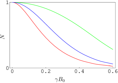
Figure 3: (Color online) Negativity $N$ in Eq. (63) as a function of $\gamma B_{0}$ for $m=100$, $p^{(\rm a)}_{0}=10$, $L=3$, and $\sigma^{(\rm a)}=1$, 2, and 3. The higher curves correspond to the thinner $\sigma$’s. All quantities are given in $0.1p_{0}^{(\rm a)}$ units.

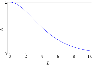
Figure 4: (Color online) Negativity $N$ in Eq. (63) as a function of $L$ for $m=100$, $p^{(\rm a)}_{0}=10$, $\gamma B_{0}=0.2$, and $\sigma^{(\rm a)}=2$. All quantities are given in $0.1p_{0}^{(\rm a)}$ units.

On the other hand, the wider $\sigma^{(\rm a)}$ the more destructive interference between ${\cal{T}}_{\uparrow}(p)$ and ${\cal{T}}_{\downarrow}(p)$ will occur, reducing $N$. We plot in Figure 3 the negativity $N$ as a function of $\gamma B_{0}$, with $B_{0}:=|{\bf{B}}_{0}|$, for $m=100$, $p^{(\rm a)}_{0}:=|{\bf{p}}^{(\rm a)}_{0}|=10$, $L=3$, and $\sigma^{(\rm a)}=1$, 2, and 3. All quantities are given in $0.1p_{0}^{(\rm a)}$ units. The entanglement goes to zero with increasing $B_{0}$, and the wider $\sigma^{(\rm a)}$, the lesser the entanglement. A similar behaviour arises from the cumulative effect of the barrier; the larger $L$, the smaller the entanglement. We show in Figure 4 this behavior, plotting $N$ as a function of $L$ for $m=100$, $p^{(\rm a)}_{0}=10$, $\gamma B_{0}=0.2$, and $\sigma^{(\rm a)}=2$.

III.2 Two photons and an optically-active medium

In this section we analyze a bipartite system, composed by two photons $A$ and $B$, which are far apart in a polarization Bell state $|\Psi^{-}\rangle$ with factorized Gaussian momentum distributions. We consider that the photon $A$ traverses a region where a finite, optically-active medium, exists. As a result, part of its spin correlations will be transferred to the momentum.

Basically the mathematical formalism used for the two-fermion case is also valid here, with $\uparrow$ and $\downarrow$ indicating right-hand and left-hand circular polarizations, which we will denote by R and L indices. The transmission coefficient in the WKB approximation, at lowest order, takes now the form of a complex phase, depending on the polarization

$${\cal{T}}_{s}(w):=\exp[iwn_{s}(w)L],\;\;\;s=R,L,$$ (64)

where the refraction indices are

$$n_{\rm R,L}(w):=\sqrt{1+\chi_{11}\pm\chi_{12}},$$ (65)

and $\chi_{11}$, $\chi_{12}$ are two of the matrix elements of the susceptibility $\chi$,

$$\chi:=\left(\begin{array}[]{ccc}\chi_{11}&i\chi_{12}&0\\ -i\chi_{12}&\chi_{11}&0\\ 0&0&\chi_{33}\end{array}\right).$$ (66)

$\chi$ is produced, for example, by an isotropic dielectric placed in a magnetic field ${\bf{B}}_{0}$ directed along $z$, which is also the direction of photon propagation. $L$ is the dielectric length that the photon traverses. $\chi_{11}$ and $\chi_{12}$ are

$$\chi_{11}(w):=\frac{{\cal{N}}e^{2}}{m\epsilon_{0}}\left[\frac{w_{0}^{2}-w^{2}}{(w_{0}^{2}-w^{2})^{2}+w^{2}w_{c}^{2}}\right],$$

$$\chi_{12}(w):=\frac{{\cal{N}}e^{2}}{m\epsilon_{0}}\left[\frac{ww_{c}}{(w_{0}^{2}-w^{2})^{2}+w^{2}w_{c}^{2}}\right],$$ (67)

where the cyclotron frequency $w_{c}:=e|{\bf{B}}_{0}|/m$, $e$ is the electron charge, $m$ its mass, $w_{0}$ the resonance frequency of the optically-active medium, ${\cal{N}}$ the number of electrons per unit volume, and $\epsilon_{0}$ the vacuum electric permittivity.

The next order correction would include factors $\sqrt{n_{\rm R,L}}$ in the denominators of the transmission coefficients. However, the approximation that considers these factors coincides exactly with the lowest order one when taking into account just linear terms in ${\bf{B}}_{0}$. We will consider the realistic case in which $w_{c}$ is small as compared to the photon average energy. Thus we will work from the very beginning just with the transmission coefficients (64).

The negativity $N$, obtained for this case in analogy with the two-fermion case, is

$$N\simeq\frac{1}{\sqrt{\pi}\sigma}\left|\int_{0}^{\infty}dwe^{-(w-p_{0})^{2}/\sigma^{2}}e^{i\tilde{B}L\frac{w^{2}}{(w^{2}-w_{0}^{2})^{2}}}\right|,$$ (68)

where $p_{0}$ is the average momentum of photon $A$, $\sigma\ll p_{0}$ its momentum width, and $\tilde{B}:={\cal N}e^{3}|{\bf{B}}_{0}|/(m^{2}\epsilon_{0})$.

We plot in Figure 5 the negativity $N$ in Eq. (68) as a function of $\tilde{B}L$ for $p_{0}=10$, $\sigma=2$, and $w_{0}=10$. All quantities are given in $0.1p_{0}$ units. The entanglement decreases as the magnetic field $\tilde{B}$ or the length $L$ of the dielectric increase. We plot also in Figure 6 the negativity $N$ as a function of $\sigma$ for $p_{0}=10$, $\tilde{B}L=4$, and $w_{0}=10$. Surprisingly, and opposite to the two-fermion case, the entanglement increases as the momentum width $\sigma$ of the photon is larger. This effect comes from the fact that for larger widths, centered at $w_{0}$, the contribution from the region around the resonance frequency $w_{0}$, in which the effect of the medium is appreciable, becomes smaller. On the other hand, in the limit of negligible width, the spin could not get entangled with the momentum so in this limit the spin-spin entanglement would remain maximal. We observe then that there is a region of intermediate widths $\sigma$ in which the spin-spin entanglement becomes minimal. Finally, we plot in Figure 7 the negativity $N$ as a function of $w_{0}$ for $p_{0}=10$, $\tilde{B}L=2$, and $\sigma=0.5,1,2$. The higher curves correspond to the wider $\sigma$’s. These graphics show that the entanglement decreases mainly for resonance frequencies $w_{0}$ around the average momentum $p_{0}$. It also shows the surprising behavior mentioned above: For wider $\sigma$, the entanglement is larger, and the interval of $w_{0}$ for which the entanglement decreases is wider, as expected according to the previous analysis.

Figure 5: (Color online) Negativity $N$ in Eq. (68) as a function of $\tilde{B}L$ for $p_{0}=10$, $\sigma=2$, and $w_{0}=10$. All quantities are given in $0.1p_{0}$ units.

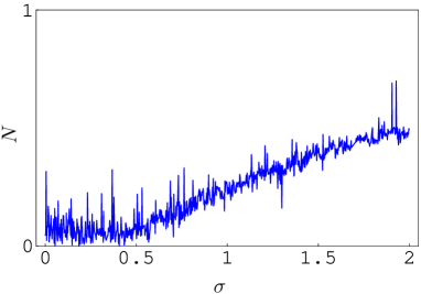
Figure 6: (Color online) Negativity $N$ in Eq. (68) as a function of $\sigma$ for $p_{0}=10$, $\tilde{B}L=4$, and $w_{0}=10$. All quantities are given in $0.1p_{0}$ units.

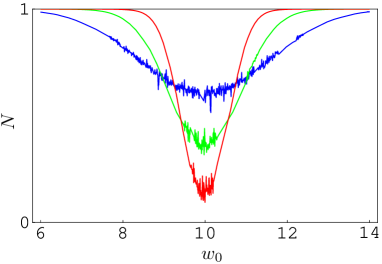
Figure 7: (Color online) Negativity $N$ in Eq. (68) as a function of $w_{0}$ for $p_{0}=10$, $\tilde{B}L=2$, and $\sigma=0.5,1,2$. The higher curves correspond to the wider $\sigma$’s. All quantities are given in $0.1p_{0}$ units.

IV IS PURELY QUANTUM COMMUNICATION FEASIBLE?

A cautious reader may immediately object that, in principle, our preceding analysis seems to suggest the feasibility of communication through a purely quantum channel, i.e. without classical communication, contrary to all known quantum-informational protocols. Let us illustrate this point with the following proposal based in the previous two-fermion case. As usual, Alice and Bob will be the corresponding observers of each fermion. The joint spin-spin state is given by equation (61), which immediately drives one to the subsequent reduced spin state for fermion $B$

$$\rho_{B}=\begin{pmatrix}I_{\downarrow\downarrow}&0\\ 0&I_{\uparrow\uparrow}\end{pmatrix}.$$ (69)

But the quantities $I_{ss^{\prime}}$ depend on the magnetic field $B_{0}$ (cf. equations (62) and (59)), which can be controlled by Alice. This allows them to agree on the following procedure. They agree on communicating with a binary alphabet with classical bits $0$ and $1$. If Alice were to communicate $0$, she would adjust $B_{0}$ so that the reduced spin state for Bob is, for example,

$$\rho_{B}^{(0)}=\begin{pmatrix}\frac{3}{4}&0\\ 0&\frac{1}{4}\end{pmatrix}.$$ (70)

They prepare a statistically significative amount of pairs of fermions under such conditions. Then Bob, when measuring the spin upon his fermion, will typically obtain spin up in the $75\%$ of the measurements and spin down in the remaining $25\%$. He thus deduces that Alice is sending the bit $0$.

On the contrary, if Alice were to communicate the bit $1$, she would adjust $B_{0}$ so that the reduced spin state for Bob is, for example,

$$\rho_{B}^{(1)}=\begin{pmatrix}\frac{1}{4}&0\\ 0&\frac{3}{4}\end{pmatrix}.$$ (71)

They also prepare a statistically significative amount of pairs and Bob performs his measurements. He will detect $75\%$ of them in the spin down state and $25\%$ in the spin up state. He thus deduces that Alice is sending the bit $1$. Notice that this information transmission is carried out without the assistance of classical communication.

The flaw stems from the disregarding of the wave packet reflection in Alice’s site. This can be seen in two complementary ways. On the one hand, to perform a genuine information transmission in which Bob’s fermion is actually carrying information encoded by Alice, he must be able to discern between those fermions whose pairs have been reflected in Alice’s barrier potential, so that he can securely discard them (they are not carrying information at all). And this is only possible if Alice classically communicates this information to Bob. On the other hand, a detailed calculation taking into account the reflection coefficients, hence without the normalization appearing in the denominator of (62), shows that Bob’s reduced spin state will be given by

$$\rho_{B} = \frac{1}{2}\begin{pmatrix}\int d^{3}\mathbf{p}|\mathcal{G}(\mathbf{p})|^{2}|\mathcal{R}_{\downarrow}(p)|^{2}&0\\ 0&\int d^{3}\mathbf{p}|\mathcal{G}(\mathbf{p})|^{2}|\mathcal{R}_{\uparrow}(p)|^{2}\end{pmatrix}$$ (72)

$$+ \frac{1}{2}\begin{pmatrix}\int d^{3}\mathbf{p}|\mathcal{G}(\mathbf{p})|^{2}|\mathcal{T}_{\downarrow}(p)|^{2}&0\\ 0&\int d^{3}\mathbf{p}|\mathcal{G}(\mathbf{p})|^{2}|\mathcal{T}_{\uparrow}(p)|^{2}\end{pmatrix}=$$

$$= \frac{1}{2}\begin{pmatrix}1&0\\ 0&1\end{pmatrix},$$

where $\mathcal{R}_{s}(p)$ denotes the corresponding reflection coefficient for spin $s$ and momentum $p$. The calculation reveals that Bob gains no information whatsoever from Alice’s decisions, unless she classically informs Bob about them.

Mathematically this can be expressed through the unitary character of the process. If no classical information is exchanged, the evolution is locally unitary ($\Psi^{(a)}\otimes\Psi^{(b)}\to U^{(a)}[\Psi^{(a)}]\otimes U^{(b)}[\Psi^{(b)}]$) and thus cannot change the entanglement shared by both parties (the entanglement is invariant under local unitary evolution). Consequently no information through the purely quantum channel can be obtained. On the contrary, if Alice classically sends information to Bob, she is actually selecting a subset of her incoming fermions, i.e. she is projecting her state ($\Psi^{(a)}\otimes\Psi^{(b)}\to P^{(ab)}[\Psi^{(a)}\otimes\Psi^{(b)}]$, where $P^{(ab)}$ is an orthogonal projector), which is a non-unitary operator which changes the entanglement class. This fact allows them to exploit the initial quantum correlations between their fermions to establish a communication protocol.

In summary, this example shows once more the impossibility of using quantum correlations, i.e. entanglement to exchange information without the aid of classical communication.

V CONCLUSIONS

We showed the spin entanglement loss by transfer of correlations to the momentum of one of the particles, through a local spin-momentum entangling interaction. This phenomenon, already analyzed for a non-interacting particular case in the context of Wigner rotations of special relativity, may produce decoherence of Bell spin states. The momentum of each particle is a very simple reservoir and indeed it is one that cannot be eliminated by improving the experimental conditions, due to Heisenberg’s principle. We show that an $s=\frac{1}{2}$ fermion (photon), which initially belongs to a Bell spin state, may lose its spin correlations due to this physical phenomenon when traversing a local magnetic field (optically-active medium). These specific media entangle each component of the spin state of the particle with its momentum, like in a Stern-Gerlach device. This could have implications for quantum communication and information processing devices.

References

- Nielsen and Chuang (2000) M. A. Nielsen and I. L. Chuang, Quantum Computation and Quantum Information (Cambridge University Press, Cambridge, 2000).
- Galindo and Martín-Delgado (2002) A. Galindo and M. A. Martín-Delgado, Rev. Mod. Phys. 74, 347 (2002).
- Yu and Eberly (2002) T. Yu and J. H. Eberly, Phys. Rev. B 66, 193306 (2002).
- Yu and Eberly (2003) T. Yu and J. H. Eberly, Phys. Rev. B 68, 165322 (2003).
- Yu and Eberly (2004) T. Yu and J. H. Eberly, Phys. Rev. Lett. 93, 140404 (2004).
- Dodd and Halliwell (2004) P. J. Dodd and J. J. Halliwell, Phys. Rev. A 69, 052105 (2004).
- Nikolić and Souma (2005) B. K. Nikolić and S. Souma, Phys. Rev. B 71, 195328 (2005).
- Carvalho et al. (2005) A. R. R. Carvalho, F. Mintert, S. Palzer, and A. Buchleitner, quant-ph/0508114 (2005).
- França Santos et al. et al. (2005) M. França Santos, P. Milman, L. Davidovich, and N. Zagury, Phys. Rev. A 73, 040305(R) (2006).
- Peres et al. (2002) A. Peres, P. F. Scudo, and D. R. Terno, Phys. Rev. Lett. 88, 230402 (2002).
- Czachor (2005) M. Czachor, Phys. Rev. Lett. 94, 078901 (2005).
- Alsing and Milburn (2002) P. M. Alsing and G. J. Milburn, Quant. Inf. Comput. 2, 487 (2002).
- Gingrich and Adami (2002) R. M. Gingrich and C. Adami, Phys. Rev. Lett. 89, 270402 (2002).
- Pachos and Solano (2003) J. Pachos and E. Solano, Quant. Inf. Comput. 3, 115 (2003).
- Czachor and Wilczewski (2003) M. Czachor and M. Wilczewski, Phys. Rev. A 68, 010302(R) (2003).
- Gingrich et al. (2003) R. M. Gingrich, A. J. Bergou, and C. Adami, Phys. Rev. A 68, 042102 (2003).
- Lamata et al. (2005) L. Lamata, M. A. Martín-Delgado, and E. Solano, quant-ph/0512081 (2005).
- Scully et al. (2005) M. O. Scully, and M. S. Zubairy, Quantum Optics (Cambridge University Press, Cambridge, 1997).
- França Santos et al. (2005) M. França Santos, P. Milman, A. Z. Khoury, and P. H. Souto Ribeiro, Phys. Rev. A 64, 023804 (2001).
- Vidal and Werner (2002) G. Vidal and R. F. Werner, Phys. Rev. A 65, 032314 (2002).
- Peres (1995) A. Peres, Quantum Theory: Concepts and Methods (Kluwer Academic Publishers, Dordrecht, 1995).