Operational Classification and Quantification of Multipartite Entangled States

Abstract

We formalize and extend an operational multipartite entanglement measure introduced in T. R. Oliveira, G. Rigolin, and M. C. de Oliveira, Phys. Rev. A 73, 010305(R) (2006) through the generalization of global entanglement (GE) [ D. A. Meyer and N. R. Wallach, J. Math. Phys. 43, 4273 (2002)]. Contrarily to GE the main feature of this new measure lies in the fact that we study the mean linear entropy of all possible partitions of a multipartite system. This allows the construction of an operational multipartite entanglement measure which is able to distinguish among different multipartite entangled states that GE failed to discriminate. Furthermore, it is also maximum at the critical point of the Ising chain in a transverse magnetic field being thus able to detect a quantum phase transition.

I Introduction

Since Schrödinger’s seminal paper schroedinger entanglement is recognized to be at the heart of Quantum Mechanics (QM). For a long time the study of entangled states was restricted to the conceptual foundations of QM epr ; bell . Since the last two decades, however, entanglement was also recognized as a physical resource which can be used to efficiently implement informational and computational tasks livrodonielsen . The understanding of the qualitative and quantitative aspects of entanglement, therefore, naturally became a fertile field of research. Nowadays, entanglement of bipartite states (a joint state of a quantum system partitioned in two subsystems $A$ and $B$) is quite well understood. Good measures of entanglement for these systems are available, specially for qubits wootters . On the other hand entanglement of multipartite states (a joint state of a quantum system partitioned in more than two subsystems) cannot be understood through simple extensions of the tools and measures employed for bipartite entangled states. Most of the tools available to study bipartite states (e.g. the Schmidt decomposition Schmidt ) are in general not useful for multipartite states. Even a qualitative characterization of the many possible multipartite entangled states (MES) is very complex since for a given $N$-partitioned system there are many “kinds” of entanglement cirac ; verschelde . For example, let $|\Psi\rangle_{N}=|\phi_{1}\rangle\otimes\cdots\otimes|\phi_{p}\rangle\otimes|\psi\rangle_{N-p}$ be a $N$-partite state in which $|\phi_{i}\rangle$, $1\leq i\leq p$, is the $i$th subsystem state and $|\psi\rangle_{N-p}$ is the state describing the other $N-p$ subsystems. If $|\psi\rangle_{N-p}$ is an entangled state then $|\Psi\rangle$ is called a $p$-separable state footnote1 . After discovering the value of $p$ for a given multipartite state another complication shows up when we focus on $|\psi\rangle_{N-p}$ since its subsystems can be entangled in several inequivalent ways. For example, in the case of three qubits there are two paradigmatic MES which cannot be converted to each other via local operations and classical communication (LOCC)cirac . For four qubits, nine different kinds of entanglement are possible, which cannot be converted to each other via LOCC verschelde . Thus after considerable work we still lack a deep understanding of MES and new tools must be developed in order to capture the essential features of genuine multipartite entanglement (ME).

Our aim in this paper is to shed new light on the way ME is characterized and quantified. We intend to do this by formalizing and extending an operational ME measure introduced in Ref. nossopaper . We emphasize that it is an operational measure in the sense that it is easily computable, even for a multipartite state composed of many subsystems. This new measure can be seen as an extension of the global entanglement and we call it, from now on, the generalized global entanglement: $E_{G}^{(n)}$. The generalized global entanglement has several interesting features, two of which were already explored in Ref. nossopaper : (i) in contrast to the global entanglement measure meyer it can identify genuine MES and (ii) it is maximum at the critical point for the Ising chain in a transverse magnetic field. Another important aspect of $E_{G}^{(n)}$ is the fact that it has an intuitive physical interpretation. We can relate it to the linear entropy of the pure state being studied as well as with the purities of the reduced $n$-party states obtained by tracing out the other $N-n$ subsystems viola ; somma .

This paper is organized as follows. In Sec. II we formally define $E_{G}^{(n)}$ and we extensively discuss a few important properties satisfied by the generalized global entanglement. In Sec. III we calculate $E_{G}^{(n)}$ for the most representatives MES. This gives us a good intuition of the meaning of $E_{G}^{(n)}$ and illustrates its usefulness. We also compare $E_{G}^{(n)}$ with other measures available, highlighting the main differences and the advantages and disadvantages of each one. In the same section we use $E_{G}^{(2)}$ to quantify the ground state multipartite entanglement of the one dimension (1D) Ising model in a transverse magnetic field. Finally, in Sec. IV we present our final remarks.

II Generalized Global Entanglement

Global entanglement (GE) was firstly introduced in Ref. meyer to quantify the ME contained in a chain of N qubits. Latter it was demonstrated brennen to be equivalent to the mean linear entropy (LE) of all single qubits in the chain. This connection between GE and LE considerably simplified the calculation of GE and also extended it to systems of higher dimensions. An intuitive, though not so rigorous, way of understanding GE is to consider it as quantifying the mean entanglement between one subsystem with the rest of the subsystems. In this process we are dividing a system of $N$ components into a single subsystem and the remaining $N-1$ subsystems. We could, nevertheless, separate the system into two partition blocks, one containing $L$ subsystems and the other one $N-L$ latorre ; latorre2 . There are many different ways to construct a given “block”. In Refs. latorre ; latorre2 a block of $L$ subsystems consisted of the first $L$ successive subsystems: $L=\{S_{1},S_{2},S_{3},\ldots,S_{L}\}$. But any other possible combination of $L$ subsystems could be employed to construct a block. We may have, for instance, a block formed by the first $L$ odd subsystems: $L=\{S_{1},S_{3},S_{5},\ldots,S_{2L-1}\}$. It is legitimate to compute the LE of each one of these possible partitions. Roughly speaking this allows us to detect and quantify all possible ‘types’ of entanglement in a multipartite pure state. The generalized global entanglement $(E_{G}^{(n)})$ is defined to take into account all of those possible partitions of a system composed of $N$ subsystems. Before we define $E_{G}^{(n)}$ we highlight two of its main important qualities: (a) It is a relatively simple and operational measure. Since it is based on LE it can be easily evaluated and it is valid for any type of multipartite pure state (states belonging either to finite or infinite dimension Hilbert spaces); (b) Each class of $E_{G}^{(n)}$ is related to the mixedness/purity of all possible $n$-partite reduced density matrices out of a system composed of $N$ subsystems, and thus it is not restricted to reduced density matrices of only one subsystem as the original GE meyer ; somma ; viola . This fact is helpful for the physical understanding of $E_{G}^{(n)}$.

Following the definition of $E_{G}^{(n)}$ we move to the study of the general properties of this new measure relating it to the mixedness/purity of the various reduced density matrices of the system. After that we particularize to qubits focusing on the ability of the generalized global entanglement to classify and quantify MES. We conclude this section by presenting a variety of examples, which clarify the necessity of all the classes of $E_{G}^{(n)}$, i. e. $n=1,2,3,\ldots$, to properly understand the many facets of MES.

II.1 Formal Definition of the Measure

Consider a system $S$ which is partitioned into $N$ subsystems $S_{i}$, $1\leq i\leq N$. Let $|\Psi\rangle\in\mathcal{H}$ be a quantum state describing $S$ and $\mathcal{H}$ the Hilbert space of the whole system. Since we have $N$ subsystems, $\mathcal{H}=\mathcal{H}_{1}\otimes\cdots\otimes\mathcal{H}_{N}=\bigotimes_{i=1}^{N}\mathcal{H}_{i}$, in which $\mathcal{H}_{i}$ is the Hilbert space associated with $S_{i}$. The density matrix of $S$ is $\rho=|\Psi\rangle\langle\Psi|$ and we define the generalized global entanglement CommentScott as,

$$E_{G}^{(n)}(\rho) = \frac{1}{C^{N-1}_{n-1}}\sum_{i_{1}=1}^{N-1}\sum_{i_{2}=i_{1}+1}^{N-1}\sum_{i_{3}=i_{2}+1}^{N-1}\cdots$$ (1)

$$\cdots\sum_{i_{n-1}=i_{n-2}+1}^{N-1}G(n,i_{1},i_{2},\ldots,i_{n-1}),$$

where all the parameters are natural numbers, $n<N$, and

$$C^{N-1}_{n-1}=\frac{(N-1)!}{(N-n)!(n-1)!}$$

is the definition of the binomial coefficient. Note that the summation is over all $i_{k}$’s, with the restriction that $1\leq i_{1}<i_{2}<\cdots<i_{n-1}\leq N-1$. We also assume $i_{0}=0$. The function $G$ is given as,

$$G(n,i_{1},i_{2},\ldots,i_{n-1})=\frac{d}{d-1}\left[1-\frac{1}{N-i_{n-1}}\sum_{j=1}^{N-i_{n-1}}\text{Tr}\left(\rho^{2}_{j,j+i_{1},j+i_{2},\ldots,j+i_{n-1}}\right)\right],$$ (2)

where $\rho_{j,j+i_{1},j+i_{2},\ldots,j+i_{n-1}}$ is obtained by tracing out all the subsystems but $S_{A}=\{S_{j},S_{j+i_{1}},S_{j+i_{2}},\ldots,S_{j+i_{n-1}}\}$ and $d=\text{min}\{\text{dim}\>S_{A},\text{dim}\>\overline{S}_{A}\}$. Here $\text{dim}\>S_{A}$ and $\text{dim}\>\overline{S}_{A}$ are, respectively, the Hilbert space dimension of the subsystem $S_{A}$ and of its complement $\overline{S}_{A}$. In resume the index $n$ is for the number of subsystems in the $A$ partition and the indexes $i_{1},i_{2},...,i_{n-1}$ are the neighborhood addressing for each of the involved subsystems.

II.2 General Properties

Eqs. (1) and (2) are valid for any multipartite pure system, even systems described by continuous variables (Gaussian states for example). The key concept behind generalized global entanglement is the fact that it is based on the linear entropy, which is an entanglement monotone easily calculated for the vast majority of pure states. Thus, by its very definition, $E_{G}^{(n)}$ and $G$ inherit all the properties satisfied by LE, including the crux of all entanglement monotones: non-increase under LOCC.

Another important concept of $E_{G}^{(n)}$ and $G$ is the introduction of classes of multipartite entanglement (ME) labeled by the index $n$. As we will see, they are all related with the many ways a multipartite state can be entangled. Moreover, a genuine $n$-partite entangled state must have non-zero $E_{G}^{(n)}$ and $G$’s for all classes $n$. Here a genuine MES means a multipartite pure entangled system in which no pure state can be defined to anyone of its subsystems. There is only one pure state describing the whole joint system. For three qubits, for instance, the states $|GHZ\rangle=(1/\sqrt{2})(|000\rangle+|111\rangle)$ and $|W\rangle=(1/\sqrt{3})(|001\rangle+|010\rangle+|100\rangle)$ are genuine MES but $|\xi\rangle=(1/\sqrt{2})(|00\rangle+|11\rangle)|0\rangle$ is not.

Let us now explicitly show how the first classes of $E_{G}^{(n)}$ look like. This will clarify the physical meaning of the measure as well as the intuitive aspects which led us to arrive at the general and formal definitions given in Eqs. (1) and (2).

II.2.1 First Class: $n=1$

When $n=1$ Eqs. (1) and (2) are the same,

$$E_{G}^{(1)}(\rho)=G(1)=\frac{d}{d-1}\left[1-\frac{1}{N}\sum_{j=1}^{N}\text{Tr}\left(\rho^{2}_{j}\right)\right],$$ (3)

and if we remember the definition of the linear entropy for the subsystem $j$ brennen ; indianos ,

$$E_{L}(\rho_{j})=\frac{d}{d-1}\left[1-\text{Tr}\left(\rho_{j}^{2}\right)\right],$$ (4)

then Eq. (3) can be written as nossopaper

$$E_{G}^{(1)}=\frac{1}{N}\sum_{j=1}^{N}E_{L}(\rho_{j})=\langle E_{L}(\rho_{j})\rangle.$$ (5)

In other words, $E_{G}^{(1)}$ is simply the mean linear entropy of all the subsystems $S_{j}$. We should mention that for qubits ($d=2$), $E_{G}^{(1)}$ was shown brennen to be exactly the Meyer and Wallach global entanglement meyer .

The physical intuition behind the study of the mean linear entropies lies in the fact that the more a state is a genuine MES the more mixed their reduced density matrices should be. However, we should not limit ourselves to evaluating the reduced density matrices of single subsystems $S_{j}$. We can take either two, or three, …, or $n$ subsystems and calculate their reduced density matrices and also calculate their mean linear entropies. This is the reason of why we introduced the other classes of generalized global entanglement.

II.2.2 Second Class: $n=2$

For $n=2$ Eqs. (1) and (2) are not identical anymore, being, nevertheless, entanglement monotones:

$$E_{G}^{(2)}(\rho) = \frac{1}{N-1}\sum_{i_{1}=1}^{N-1}G(2,i_{1}),$$ (6)

$$G(2,i_{1}) = \frac{d}{d-1}\left[1-\frac{1}{N-i_{1}}\sum_{j=1}^{N-i_{1}}\text{Tr}\left(\rho^{2}_{j,j+i_{1}}\right)\right].$$ (7)

Now we deal with the reduced joint density matrix for subsystems $S_{j}$ and $S_{j+i_{1}}$. The extra parameter $i_{1}$ is introduced to take account of the many possible ‘distances’ between the two subsystems. For nearest neighbors $i_{1}=1$, next-nearest neighbors $i_{2}=2$, and so forth.

Noticing that the linear entropy of the subsystems $S_{j}$ and $S_{j+i_{1}}$ by tracing out the rest of the other subsystems is given by

$$E_{L}(\rho_{j,j+i_{1}})=\frac{d}{d-1}\left[1-\text{Tr}\left(\rho_{j,j+i_{1}}^{2}\right)\right],$$ (8)

then Eq. (7) can be written as,

$$G(2,i_{1})=\frac{1}{N-i_{1}}\sum_{j=1}^{N-i_{1}}E_{L}(\rho_{j,j+i_{1}})=\langle E_{L}(\rho_{j,j+i_{1}})\rangle.$$ (9)

This implies that Eq. (6) is simply given by

$$E_{G}^{(2)}(\rho)=\frac{1}{N-1}\sum_{i_{1}=1}^{N-1}\langle E_{L}(\rho_{j,j+i_{1}})\rangle=\langle\langle E_{L}(\rho_{j,j+i_{1}})\rangle\rangle,$$ (10)

where the double brackets represent the averaging over all possible $G(2,i_{1})$, $1\leq i_{1}\leq N-1$.

Looking at Eqs. (9) and (10) we can easily interpret $E_{G}^{(2)}$ and $G(2,i_{1})$. First, let us deal with $G(2,i_{1})$. We assume that all the subsystems are organized in a linear chain. (This assumption simplifies the discussion in what follows.) If we remember that $1\leq i_{1}\leq N-1$, where $N$ is the number of subsystems, Eq. (9) tells us that $G(2,i_{1})$ is nothing but the mean linear entropy of two subsystems with the rest of the other subsystems conditioned on that these two subsystems are $i_{1}$ lattice sites apart.

For concreteness, let us explicitly write all the possible $G(2,i_{1})$ for a linear chain of five subsystems. Since $N=5$ we have $1\leq i_{1}\leq 4$, which gives four $G$’s pictorially represented in Fig. 1:

• $G(2,1)$, which is the mean linear entropy (LE) of the following pairs of subsystems with the rest of the chain: $\{(S_{1},S_{2}),(S_{2},S_{3}),(S_{3},S_{4}),(S_{4},S_{5})\}$;

• $G(2,2)$, which is the mean LE of the following pairs of subsystems: $\{(S_{1},S_{3}),(S_{2},S_{4}),(S_{3},S_{5})\}$;

• $G(2,3)$, which is the mean LE of the following pairs of subsystems: $\{(S_{1},S_{4}),(S_{2},S_{5})\}$;

• $G(2,4)$, which is the mean LE of the following pairs of subsystems: $\{(S_{1},S_{5})\}$.

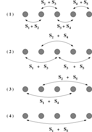
Figure 1: All combinations of two elements out of five.

Finally, Eq. (10) shows that $E_{G}^{(2)}$ is the mean linear entropy of two subsystems with the rest of the chain irrespective of the distance between the two subsystems, i.e., it is the averaged summation of all the (1)-(4) kinds of $G(2,i_{1})$, $1\leq i_{1}\leq 4$.

II.2.3 Third Class: $n=3$

By setting $n=3$ Eqs. (1) and (2) become

$$E_{G}^{(3)}(\rho)=\frac{2}{(N-1)(N-2)}\sum_{i_{1}=1}^{N-1}\sum_{i_{2}=i_{1}+1}^{N-1}G(n,i_{1},i_{2}),$$ (11)

and

$$G(3,i_{1},i_{2})=\frac{d}{d-1}\left[1-\frac{1}{N-i_{2}}\sum_{j=1}^{N-i_{2}}\text{Tr}\left(\rho^{2}_{j,j+i_{1},j+i_{2}}\right)\right].$$ (12)

Eq. (12) deals with reduced density matrices of three subsystems: $S_{j}$, $S_{j+i_{1}}$, and $S_{j+i_{2}}$. Therefore, $G(3,i_{1},i_{2})$ is the mean linear entropy of all three subsystems with the rest of the chain conditioned to that $S_{j+i_{1}}$ and $S_{j+i_{2}}$ are, respectively, $i_{1}$ and $i_{2}$ lattice sites apart from $S_{j}$. Taking the mean of all possible $G(3,i_{1},i_{2})$ we obtain Eq. (11). This is equivalent to averaging over all linear entropies of three subsystems irrespective of their distances. Although we do not explicitly write them here, similar expressions as those given by Eqs. (9) and (10) can be obtained for this class.

Again, as we did for the second class, it is explanatory to analyze in details the $N=5$ case. Now $1\leq i_{1}<i_{2}\leq 4$. This time we have six $G$’s (See Fig. 2):

• $G(3,1,2)$, which is the mean linear entropy (LE) of the following triples of subsystems with the rest of the chain: $\{(S_{1},S_{2},S_{3}),(S_{2},S_{3},S_{4}),(S_{3},S_{4},S_{5})\}$;

• $G(3,1,3)$, which is the mean LE of the following triples of subsystems: $\{(S_{1},S_{2},S_{4}),(S_{2},S_{3},S_{5})\}$;

• $G(3,1,4)$, which is the mean LE of the following triples of subsystems: $\{(S_{1},S_{2},S_{5})\}$;

• $G(3,2,3)$, which is the mean LE of the following triples of subsystems: $\{(S_{1},S_{3},S_{4}),(S_{2},S_{4},S_{5})\}$;

• $G(3,2,4)$, which is the mean LE of the following triples of subsystems: $\{(S_{1},S_{3},S_{5})\}$;

• $G(3,3,4)$, which is the mean LE of the following triples of subsystems: $\{(S_{1},S_{4},S_{5})\}$.

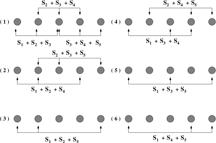
Figure 2: All combinations of three elements out of five.

II.2.4 Higher Classes: $n\geq 4$

Remembering that $n<N$, higher classes $n$ of $E_{G}^{(n)}(\rho)$ only make sense for systems such that $N\geq n+1$ subsystems. The higher a class $n$ the greater the number of $G$’s necessary for the computation of $E_{G}^{(n)}(\rho)$. This is a satisfactory property we should expect from a useful multipartite entanglement measure since as we increase the number of partitions of a system we increase the way it may be entangled cirac ; verschelde .

If we employ the definition of LE for $n$ subsystems out of a total of $N$,

$$E_{L}(\rho_{j,\ldots,j+i_{n-1}})=\frac{d}{d-1}\left[1-\text{Tr}\left(\rho_{j,\ldots,j+i_{n-1}}^{2}\right)\right],$$ (13)

we can write Eqs. (2) and (1) respectively as

$$G(n,i_{1},\ldots,i_{n-1}) = \langle E_{L}(\rho_{j,j+i_{1},\ldots,i_{n-1}})\rangle,$$ (14)

$$E_{G}^{(n)}(\rho) = \langle\langle E_{L}(\rho_{j,j+i_{1},\ldots,i_{n-1}})\rangle\rangle.$$ (15)

In Eq. (14) the single pair of brackets $\langle\;\rangle$ represents the averaging over all possible configurations of $n$ subsystems in which subsystem $S_{j+i_{k}}$ is $i_{k}$ lattice sites apart from $S_{j}$. Here $1<k<n-1$. Finally, the double brackets $\langle\langle\;\rangle\rangle$ is the average of the linear entropy of $n$ subsystems over all possible combinations (distances) in which they can be arranged.

We should mention at this point that $E_{G}^{(n)}$ and $G$ are more general than the block entanglement ($E_{B}^{(n)}$) as presented in Refs. scott ; latorre ; latorre2 . By block entanglement it is understood that we divide a set of $N$ subsystems $\{S_{1},S_{2},\ldots,S_{N}\}$ in two blocks, $A_{n}=\{S_{1},S_{2},\ldots,S_{n}\}$ and $B_{N-n}=\{S_{n+1},S_{n+2},\ldots,S_{N}\}$, and calculate the linear or von Neumann entropy between blocks $A_{n}$ and $B_{N-n}$. In the language of generalized global entanglement, block entanglement for a translational symmetric state is simply

$$E_{B}^{(n)}=G(n,i_{1}=1,i_{2}=1,\ldots,i_{n-1}=1),$$

which is only one of the many $G$’s we can define. The main difference between these two measures lies in the fact that we allow all possible combinations of $n$ subsystems out of $N$ to represent a possible ‘block’. Contrarily to block entanglement, here there exists no restriction onto the subsystems belonging to a given ‘block’ to be nearest neighbors. They lie anywhere in the system’s domain.

II.3 Particular Properties for Qubits

Although Eqs. (1) and (2) are defined for Hilbert spaces of arbitrary dimensions we now focus on some properties of $E_{G}^{(n)}$ and $G$ for qubits. There are two main reasons for studying qubits in detail. Firstly, they are recognized as a key concept for quantum information theory and secondly, the simplest multipartite states are constructed employing qubits.

Let $\rho=|\Psi\rangle\langle\Psi|$ be the density matrix of a $N$ qubit system and $\rho_{j}=\text{Tr}_{\overline{j}}(\rho)$ the reduced density matrix of subsystem $S_{j}$, which is obtained by tracing out all subsystems but $S_{j}$. A general one qubit density matrix can be written as

$$\rho_{j}=\text{Tr}_{\overline{j}}(\rho)=\frac{1}{2}\sum_{\alpha}p^{\alpha}_{j}\sigma_{j}^{\alpha},$$ (16)

where the coefficients are given by

$$p^{\alpha}_{j}=\text{Tr}\left(\sigma_{j}^{\alpha}\rho_{j}\right)=\langle\Psi|\sigma_{j}^{\alpha}|\Psi\rangle.$$ (17)

Here $\sigma_{j}^{\alpha}$ is the Pauli matrix acting on the site $j$, $\alpha=0,x,y,z$, where $\sigma^{0}$ is the identity matrix of dimension two, and $p^{\alpha}_{j}$ is real. Since $\rho_{j}$ is normalized $p_{0}=1$. Using Eqs. (16) and (17) we obtain

$$\text{Tr}\left(\rho_{j}^{2}\right)=\frac{1}{2}\left(1+\langle\sigma^{x}_{j}\rangle^{2}+\langle\sigma^{y}_{j}\rangle^{2}+\langle\sigma^{z}_{j}\rangle^{2}\right).$$ (18)

This last result implies that Eq. (3) can be written as

$$E_{G}^{(1)}=1-\frac{1}{N}\sum_{j=1}^{N}\left(\langle\sigma^{x}_{j}\rangle^{2}+\langle\sigma^{y}_{j}\rangle^{2}+\langle\sigma^{z}_{j}\rangle^{2}\right).$$ (19)

One interesting situation occurs when we have translational invariant states $\rho$. (The Ising model ground state for example.) In this scenario $\langle\sigma_{i}^{\alpha}\rangle=\langle\sigma_{j}^{\alpha}\rangle$ for any $i$ and $j$. Therefore, Eq. (19) becomes

$$E_{G}^{(1)}=1-\langle\sigma^{x}_{j}\rangle^{2}-\langle\sigma^{y}_{j}\rangle^{2}-\langle\sigma^{z}_{j}\rangle^{2},$$ (20)

which is related to the total magnetization $M$ of the system, $|M|^{2}=N(\langle\sigma_{j}^{x}\rangle^{2}+\langle\sigma_{j}^{y}\rangle^{2}+\langle\sigma_{j}^{z}\rangle^{2})$, by $E_{G}^{(1)}=1-\frac{|M|^{2}}{N}$.

By tracing out all subsystems but $S_{i}$ and $S_{j}$ we obtain the two qubit reduced density matrix

$$\rho_{ij}=\text{Tr}_{\overline{ij}}(\rho)=\frac{1}{4}\sum_{\alpha,\beta}p^{\alpha\beta}_{ij}\sigma_{i}^{\alpha}\otimes\sigma_{j}^{\beta},$$ (21)

where

$$p^{\alpha\beta}_{ij}=\text{Tr}\left(\sigma_{i}^{\alpha}\sigma_{j}^{\beta}\rho_{ij}\right)=\langle\Psi|\sigma_{i}^{\alpha}\sigma_{j}^{\beta}|\Psi\rangle.$$ (22)

Eq. (21) is the most general way to represent a two-qubit state and together with Eq. (22) imply that

$$\text{Tr}\left(\rho_{ij}^{2}\right)=\frac{1}{4}\sum_{\alpha,\beta}\langle\sigma_{i}^{\alpha}\sigma_{j}^{\beta}\rangle^{2}.$$ (23)

Remark that in Eq. (23) the trace of $\rho_{ij}^{2}$ is the sum of all one and two-point correlation functions. Moreover, since $E_{G}^{2}$ and $G(2,i_{1})$ depend on Eq. (23), we find in these entanglement measures both diagonal and off-diagonal correlation functions.

Again it is instructive to study translational symmetric states in which $p_{ij}^{\alpha\beta}=p_{ij}^{\beta\alpha}$ for any $\alpha$ and $\beta$. Using this assumption in Eq. (7) we get

$$G(2,i_{1}) = 1-\frac{2}{3}\left[\langle\sigma_{j}^{x}\rangle^{2}+\langle\sigma_{j}^{y}\rangle^{2}+\langle\sigma_{j}^{z}\rangle^{2}+\langle\sigma_{j}^{x}\sigma_{j+i_{1}}^{y}\rangle^{2}\right.$$ (24)

$$+\langle\sigma_{j}^{x}\sigma_{j+i_{1}}^{z}\rangle^{2}+\langle\sigma_{j}^{y}\sigma_{j+i_{1}}^{z}\rangle^{2}+\langle\sigma_{j}^{x}\sigma_{j+i_{1}}^{x}\rangle^{2}/2$$

$$\left.+\langle\sigma_{j}^{y}\sigma_{j+i_{1}}^{y}\rangle^{2}/2+\langle\sigma_{j}^{z}\sigma_{j+i_{1}}^{z}\rangle^{2}/2\right].$$

Note that the previous formula is not valid for $N\leq 3$. For $N=2$ only $E_{G}^{(1)}$ is defined and for $N=3$ we have $d=\text{min}\{\text{dim}\>S_{A},\text{dim}\>\overline{S}_{A}\}=2$ and not $d=4$, the value of $d$ for all $N\geq 4$. Now if we compare $G(2,i_{1})$ with the concurrence (a bipartite entanglement monotone), as we do for the Ising model in Sec. III.2, we will note that while the concurrence does not depend on any one-point and on any off-diagonal two-point correlation function nome_dificil1 ; nome_dificil2 $G(2,i_{1})$ does.

II.4 Why Do We Need Higher Classes?

The simple fact that different types of entanglement appear as we increase the number of qubits (or equivalently the number of subsystems) cirac ; verschelde indicates that the various classes here introduced may be useful to classify and quantify the many facets of ME. For example, the first class $E_{G}^{(1)}$ does not suffice to unequivocally quantify MES. Although it is maximal for Greenberger-Horne-Zeilinger (GHZ) states ghz it is also maximal for a state which is not a MES, as we now demonstrate. Let us compute $E_{G}^{(1)}$ for three paradigmatic multipartite states. The first one is the GHZ state:

$$|GHZ_{N}\rangle=\frac{1}{\sqrt{2}}\left(|0\rangle^{\otimes N}+|1\rangle^{\otimes N}\right),$$ (25)

where $|0\rangle^{\otimes N}$ and $|1\rangle^{\otimes N}$ represent, respectively, $N$ tensor products of the states $|0\rangle$ and $|1\rangle$. The GHZ state is a genuine MES since by measuring only one of the qubits in the standard basis we know exactly the results of the other $N-1$ qubits. Furthermore, tracing out any one of the qubits we obtain a separable state. A direct calculation gives $E_{G}^{(1)}(GHZ_{N})=1$.

The second state we shall analyze is given by a tensor product of $N/2$ Einstein-Podolsky-Rosen (EPR) Bell states viola :

$$|EPR_{N}\rangle=|\Phi^{+}\rangle\otimes\cdots\otimes|\Phi^{+}\rangle=|\Phi^{+}\rangle^{\otimes\frac{N}{2}},$$ (26)

where $|\Phi^{+}\rangle=(1/\sqrt{2})(|00\rangle+|11\rangle)$. For definiteness, we chose one specific Bell state. However, the results here derived are quite general and valid for any $N/2$ tensor products of Bell states. This state is obviously not a genuine MES. Only the pairs of qubits $(2j-1,2j)$, where $j=1,2,...,N$, are entangled. Nevertheless, we again obtain $E_{G}^{(1)}(EPR_{N})=1$. This last result illustrates that $E_{G}^{(1)}$ being maximal is not a sufficient condition to detect genuine MES. Note that $E_{G}^{(1)}$ for both the $GHZ_{N}$ and $EPR_{N}$ states are independent of the number of qubits $N$ in the chain.

The last state we consider is the W state cirac . It is defined as,

$$|W_{N}\rangle=\frac{1}{\sqrt{N}}\sum_{j=1}^{N}|000\cdots 1_{j}\cdots 000\rangle.$$ (27)

The state $|000\cdots 1_{j}\cdots 000\rangle$ represents a $N$ qubit state in which the $j$-th qubit is $|1\rangle$ and all the others are $|0\rangle$. As shown in Ref. meyer , $E_{G}^{(1)}(W_{N})=4(N-1)/N^{2}$. Note that $E_{G}^{(1)}$ depends on $N$ and at the thermodynamic limit ($N\rightarrow\infty$) we have $E_{G}^{(1)}(W_{N})=0$. For three qubits, the W state was shown cirac to be a genuine MES not convertible via LOCC to a GHZ state.

The computation of $E_{G}^{(2)}$ and $G(2,1)$ give different values for each of those states. Remark that for $N=2$ the previous functions are not defined and that for $N=3$ $E_{G}^{(2)}=G(2,1)=1$. Table 1 shows $E_{G}^{(2)}$ and $G(2,1)$ for the states $GHZ_{N},EPR_{N}$, and $W_{N}$. We should mention that due to translational symmetry, $G(2,1)$ and $E_{G}^{(2)}$ are identical for the states $GHZ_{N}$ and $W_{N}$.

Table 1: The third and fourth columns give $G(2,1)$ and $E_{G}^{(2)}$ for the three states listed in the first column when $N>3$. The second column gives $E_{G}^{(1)}$ for all $N$. Contrary to $E_{G}^{(1)}$, we see that $G(2,1)$ and $E_{G}^{(2)}$ distinguish the three states from each other.

	$E_{G}^{(1)}$	$G(2,1)$	$E_{G}^{(2)}$
$GHZ_{N}$	$1$	$\frac{2}{3}$	$\frac{2}{3}$
$EPR_{N}$	$1$	$\frac{N-2}{2(N-1)}$	$\frac{(2N-1)(N-2)}{2(N-1)^{2}}$
$W_{N}$	$\frac{4(N-1)}{N^{2}}$	$\frac{16(N-2)}{3N^{2}}$	$\frac{16(N-2)}{3N^{2}}$

It is interesting to note that depending on the value of $N$, the states are differently classified through $G(2,1)$. Fig. 3 illustrates the behavior of $G(2,1)$ for those three paradigmatic state as we vary $N$.

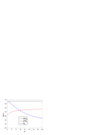
Figure 3: (Color online) Here we show $G(2,1)$ as a function of the number of qubits $N$ for the states $GHZ_{N}$, $EPR_{N}$ and $W_{N}$. Note that only when $N=4$ we have two states with the same entanglement. Furthermore, for $4\leq N\leq 8$, $W_{N}$ is more entangled than $EPR_{N}$. This ordering is changed for $N\geq 9$.

A similar behavior is observed for $E_{G}^{(2)}$ (Fig. 4). In this case, however, $EPR_{N}$ is the most entangled state for long chains. The reason for this lies in the definition of $E_{G}^{(2)}$. For the $EPR_{N}$ state, $G(2,l)$ = 1 for any $l\geq 2$. Therefore, since $E_{G}^{(2)}$ is obtained averaging over all $G(2,l)$, for long chains $G(2,1)$ does not contribute much and $E_{G}^{(2)}\rightarrow 1$.

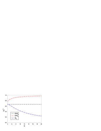
Figure 4: (Color online) Here we show $E_{G}^{(2)}$ as a function of $N$. Again, only when $N=4$ we have two states with the same entanglement. Moreover, for $N\geq 4$, $EPR_{N}$ is the most entangled state.

We also calculated the values of $E_{G}^{(1)}$, $E_{G}^{(2)}$, and $G(2,1)$ at the thermodynamic limit. See Tab. 2.

Table 2: $E_{G}^{(1)}$, $G(2,1)$, and $E_{G}^{(2)}$ at the thermodynamic limit.

$N\rightarrow\infty$	$E_{G}^{(1)}$	$G(2,1)$	$E_{G}^{(2)}$
$GHZ_{N}$	$1$	$2/3$	$2/3$
$EPR_{N}$	$1$	$1/2$	$1$
$W_{N}$	$0$	$0$	$0$

Thus even at the thermodynamic limit $E_{G}^{(2)}$ and $G(2,1)$ distinguish the three states. The ordering of the states, nevertheless, is different. Again this is related to the definition of $E_{G}^{(2)}$ and is due to the contribution of $G(2,l)$, $l\geq 2$, in the calculation of $E_{G}^{(2)}(EPR_{N})$.

Besides a measure of multipartite entanglement being able to distinguish different kinds of states it should not differentiate states that essentially contain the same amount of entanglement. For example, let us consider the following state,

$$|EPR_{2}\rangle = |\Phi^{+}\rangle_{12}|\Phi^{+}\rangle_{34}$$ (28)

$$= \frac{1}{2}(|0\rangle_{1}|0\rangle_{2}|0\rangle_{3}|0\rangle_{4}+|0\rangle_{1}|0\rangle_{2}|1\rangle_{3}|1\rangle_{4}$$

$$+|1\rangle_{1}|1\rangle_{2}|0\rangle_{3}|0\rangle_{4}+|1\rangle_{1}|1\rangle_{2}|1\rangle_{3}|1\rangle_{4}).$$

This state describes a pair of EPR states where subsystem $S_{1}$ is entangled with $S_{2}$ and $S_{3}$ is entangled with $S_{4}$. Consider now the state defined as rigolintele

$$|g_{1}\rangle = \frac{1}{2}(|0\rangle_{1}|0\rangle_{2}|0\rangle_{3}|0\rangle_{4}+|0\rangle_{1}|1\rangle_{2}|0\rangle_{3}|1\rangle_{4}$$ (29)

$$+|1\rangle_{1}|0\rangle_{2}|1\rangle_{3}|0\rangle_{4}+|1\rangle_{1}|1\rangle_{2}|1\rangle_{3}|1\rangle_{4})$$

$$= \frac{1}{2}(|0\rangle_{1}|0\rangle_{3}|0\rangle_{2}|0\rangle_{4}+|0\rangle_{1}|0\rangle_{3}|1\rangle_{2}|1\rangle_{4}$$

$$+|1\rangle_{1}|1\rangle_{3}|0\rangle_{2}|0\rangle_{4}+|1\rangle_{1}|1\rangle_{3}|1\rangle_{2}|1\rangle_{4})$$

$$= |\Phi^{+}\rangle_{13}|\Phi^{+}\rangle_{24},$$

which is also a pair of EPR states. This time, however, subsystem $S_{1}$ is entangled with $S_{3}$ and subsystem $S_{2}$ is entangled with $S_{4}$ (See Fig. 5).

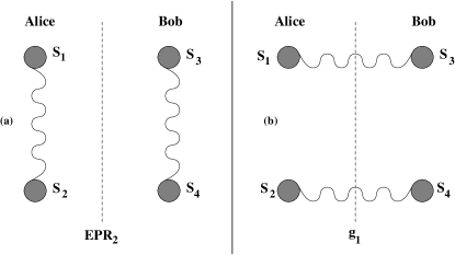
Figure 5: Pictorial representations of the states (a) $EPR_{2}$ and (b) $g_{1}$.

Although different pairs of subsystems are entangled in these two different states, their amount of entanglement is the same: there are two EPR states in both cases. This fact is captured by the entanglement measures here introduced, i.e. $E_{G}^{(n)}(EPR_{2})=E_{G}^{(n)}(g_{1})$. The block entanglement, nevertheless, does not always give the same value for the two states above (see Tab. 3).

Table 3: Comparison between $E_{G}^{(n)}$, $G(2,1)$, and $E_{B}^{(n)}$

	$E_{G}^{(1)}$	$E_{G}^{(2)}$	$G(2,1)$	$E_{B}^{(1)}$	$E_{B}^{(2)}$
$EPR_{2}$	$1$	$7/9$	$1/3$	$1$	$0$
$g_{1}$	$1$	$7/9$	$1/3$	$1$	$1$

This example illustrates that the block entanglement, as its name suggests, quantifies only the entanglement of partition $A$ (sites $1$ and $2$) with partition $B$ (sites $3$ and $4$). The generalized global entanglement $E_{G}^{(n)}$, however, quantifies the amount of entanglement of a state independently on the way it is distributed among the subsystems. We can go further and show the importance of using higher classes $E_{G}^{(n)}$ to correctly quantify the entanglement of a multipartite state no matter how the entanglement is distributed among the subsystems. For example, consider the state

$$|GHZ_{N}^{M}\rangle=|GHZ_{N}\rangle^{\otimes M},$$ (30)

where the integer $M\geq 1$ represents how many tensor products of $GHZ_{N}$ we have. Restricting ourselves to $N=3$ and $M=2$ we get,

$$|GHZ_{3}^{2}\rangle = \frac{1}{\sqrt{2}}\left(|000\rangle+|111\rangle\right)\otimes\frac{1}{\sqrt{2}}\left(|000\rangle+|111\rangle\right)$$ (31)

$$= \frac{1}{2}(|000000\rangle+|000111\rangle+|111000\rangle$$

$$+|111111\rangle).$$

Here, subsystems $S_{1}$, $S_{2}$, and $S_{3}$ form a genuine MES and $S_{4}$, $S_{5}$, and $S_{6}$ another one. For this state $E_{B}^{(3)}(GHZ^{2}_{3})=0$. If we interchange the second qubit ($S_{2}$) with the fifth one ($S_{5}$) we obtain the following state:

$$|ZHG_{3}^{2}\rangle = \frac{1}{2}(|000000\rangle+|010101\rangle+|101010\rangle$$ (32)

$$+|111111\rangle).$$

Now subsystems $S_{1}$, $S_{3}$, and $S_{5}$ form a genuine MES and $S_{2}$, $S_{4}$, and $S_{6}$ another one (See Fig. 6).

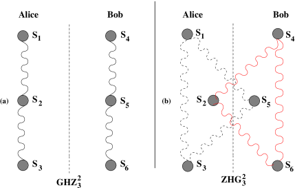
Figure 6: (Color online) Pictorial representations of the states (a) $GHZ^{2}_{3}$ and (b) $ZHG^{2}_{3}$.

Those two states have the same amount of entanglement, i. e. two GHZ states. However, the computation of the block entanglement gives $E_{B}^{(3)}(ZHG_{3}^{2})=6/7\neq E_{B}^{(3)}(GHZ^{2}_{3})$. Had we employed the generalized global entanglement we would have obtained $E_{G}^{(3)}(GHZ^{2}_{3})=E_{G}^{(3)}(ZHG_{3}^{2})$ instead. In general we have $E_{B}^{(n)}(GHZ^{2}_{n})\neq E_{B}^{(n)}(ZHG_{n}^{2})$ and $E_{G}^{(n)}(GHZ^{2}_{n})=E_{G}^{(n)}(ZHG_{n}^{2})$. Therefore, if we want to study the amount of entanglement of a multipartite state, independently on how it is distributed among the subsystems, we should employ $E_{G}^{(n)}$ instead of $E_{B}^{(n)}$, since the later furnishes only the amount of entanglement between a particular two block-partition in which the system can be divided.

III Usefulness of the Generalized Global Entanglement

In this section we present two examples in which we explore the ability of $E_{G}^{(n)}$ and the auxiliary measure $G(n,i_{1},i_{2},\ldots,i_{n-1})$ to quantify multipartite entanglement. The first example deals with a finite chain of four qubits. We show that $E_{G}^{(2)}$ together with $G(2,1)$ allow us to correctly identify MES. Moreover, comparing the values of $G(2,i_{1})$ for all the MES here presented we are led to a practical definition of what is a genuine MES. In the second example we investigate the entanglement properties of the Ising model ground state. We show that $E_{G}^{(2)}$ and $G(2,i_{1})$ are maximal at the critical point and we analyze what correlation functions are responsible for this behavior of the generalized global entanglement. The results herein presented suggest that the long range correlations in the critical point for the Ising model are related to genuine MES.

III.1 Finite Chains

Let us now focus on the simplest non-trivial spin-1/2 chain, i. e. states with $N=4$ qubits, by studying the entanglement properties of four genuine MES osterloh ; chua . The first one osterloh is the famous four qubit GHZ state ghz ,

$$|GHZ_{4}\rangle=|\Phi_{1}\rangle=\frac{1}{\sqrt{2}}\left(|0000\rangle+|1111\rangle\right).$$ (33)

Qualitative and quantitative features of this state were already discussed in Sec. II.4. A direct calculation gives $E_{G}^{(1)}\left(\Phi_{1}\right)=1;E_{G}^{(2)}\left(\Phi_{1}\right)=G(2,i_{1})\left(\Phi_{1}\right)=2/3,$ where $i_{1}=1,2,3$. The second state osterloh is written as,

$$|\Phi_{2}\rangle = \frac{1}{\sqrt{6}}\left(\sqrt{2}|1111\rangle+|1000\rangle+|0100\rangle+|0010\rangle\right.$$ (34)

$$\left.+|0001\rangle\right).$$

Calculating its first and second order generalized global entanglement we obtain $E_{G}^{(1)}\left(\Phi_{2}\right)=1;E_{G}^{(2)}\left(\Phi_{2}\right)=G(2,i_{1})\left(\Phi_{2}\right)=8/9.$ Note that as well as $|\Phi_{1}\rangle$ this state is a translational symmetric state. Moreover, $G(2,i_{1})(\Phi_{2})\geq G(2,i_{1})(\Phi_{1})$. This last result will turn out to be very useful in constructing an operational definition of MES. The third state osterloh is given as,

$$|\Phi_{3}\rangle=\frac{1}{2}\left(|1111\rangle+|1100\rangle+|0010\rangle+|0001\rangle\right).$$ (35)

Since this state is not translational symmetric, $G(2,i_{1})$ are not all equal. After a straightforward calculation we obtain $E_{G}^{(1)}\left(\Phi_{3}\right)=1;E_{G}^{(2)}\left(\Phi_{3}\right)=25/27;G(2,1)\left(\Phi_{3}\right)=7/9;G(2,2)\left(\Phi_{3}\right)=G(2,3)\left(\Phi_{3}\right)=1.$ Again we should note that $G(2,i_{1})(\Phi_{3})\geq G(2,i_{1})(\Phi_{1})$.

These three states have in common a few remarkable properties osterloh : (a) The local density operator describing each qubit is the maximally mixed state $(1/2)I_{2}$, where $I_{2}$ is the $2\times 2$ identity matrix, thus explaining why $E_{G}^{(1)}=1$ for all of them. (b) The two- and three-qubits reduced operators do not have any $k$-tangle coffman , $k=2,3$. This emphasizes that they all are genuine MES, i. e. there is no pairwise or triplewise entanglement. (c) They cannot be transformed into one another by LOCC.

We shall consider a fourth state,

$$|\chi\rangle = \frac{1}{2\sqrt{2}}\left(|0000\rangle-|0011\rangle-|0101\rangle+|0110\rangle\right.$$ (36)

$$\left.+|1001\rangle+|1010\rangle+|1100\rangle+|1111\rangle\right),$$

recently introduced and extensively studied in Ref. chua . The main feature of this state lies in its usefulness to teleport an arbitrary two-qubit state. Employing $\chi$ this task can be accomplished either from subsystems $S_{1}$ and $S_{2}$ to $S_{3}$ and $S_{4}$ or from $S_{1}$ and $S_{3}$ to $S_{2}$ and $S_{4}$. The usual channel (two Bell states) used to teleport an arbitrary two-qubit state rigolintele ; guo can teleport two qubits only from a specific location to another one: from $S_{1}$ and $S_{2}$ to $S_{3}$ and $S_{4}$ for example. In addition state $|\chi\rangle$ has a hybrid behavior in the sense that it resembles both the $GHZ$ and $W$ states chua . Tracing out any one of the qubits the remaining reduced density matrix $\sigma$ has maximal entropy, a characteristic of the $GHZ$ state. However, $\sigma$ has a non-zero negativity negativity between one qubit and the other two chua , a property of the $W$ state. By calculating the generalized global entanglement we obtain $E_{G}^{(1)}\left(\chi\right)=1;E_{G}^{(2)}\left(\chi\right)=23/27;G(2,1)\left(\chi\right)=8/9;G(2,2)\left(\chi\right)=1;G(2,3)\left(\chi\right)=2/3.$ Again we see that for all $i_{1}$ we have $G(2,i_{1})(\chi)\geq G(2,i_{1})(\Phi_{1})$.

We have grouped in Tab. 4 the entanglement calculated for the previous four states.

Table 4: Calculated values of $E_{G}^{(n)}$ and $G(2,i_{1})$ for the genuine MES shown in Sec. III.1 and for the $EPR_{2}$ state.

	$E_{G}^{(1)}$	$E_{G}^{(2)}$	$G(2,1)$	$G(2,2)$	$G(2,3)$
$EPR_{2}$	$1$	$7/9\approx 0.778$	$1/3$	$1$	$1$
$\Phi_{1}$	$1$	$2/3\approx 0.667$	$2/3$	$2/3$	$2/3$
$\Phi_{2}$	$1$	$8/9\approx 0.889$	$8/9$	$8/9$	$8/9$
$\Phi_{3}$	$1$	$25/27\approx 0.926$	$7/9$	$1$	$1$
$\chi$	$1$	$23/27\approx 0.852$	$8/9$	$1$	$2/3$

It is clear then that $E_{G}^{(1)}$ cannot be considered as the last word concerning the quantification and classification of MES. A glimpse of the first column in Tab. 4 shows that all the five states listed have $E_{G}^{(1)}=1$, even the $EPR_{2}$ state, an obvious non-genuine MES. Therefore, since $E_{G}^{(1)}=1$ is not useful to classify different genuine MES or to correctly identify them we are compelled to go further and study the higher classes of the generalized global entanglement in order to achieve such a goal. Turning our attention to $E_{G}^{(2)}$ we see that it is different for all the five states listed in Tab. 4, implying that $E_{G}^{(2)}$ can distinguish among the five states. According to $E_{G}^{(2)}$ the most entangled state is $\Phi_{3}$, which was shown to be a genuine MES osterloh .

Moreover, important clues for the understanding of what kind of entanglement is present in a given multipartite state are also available in $G(2,i_{1})$, $i_{1}=1,2,3$. Actually, these auxiliary entanglement measures give us a more detailed view of the types of entanglement a state has than $E_{G}^{(2)}$ since the latter is an average over all $G(2,i_{1})$. For example, if we relied only on $E_{G}^{(2)}$ to decide whether or not a state is a genuine MES we would arrive at a wrong answer. This point is clearly demonstrated if we compare $E_{G}^{(2)}$ for the states $EPR_{2}$ and $\Phi_{1}$ ($GHZ_{4}$). Looking at Tab. 4 we see that $E_{G}^{(2)}(EPR_{2})>E_{G}^{(2)}(\Phi_{1})$, where $EPR_{2}$ is not a genuine MES. The averaging process, as explained in Sec. II.4, is responsible for this relatively high value of $E_{G}^{(2)}$ for the state $EPR_{2}$. Remark that for translational symmetric states $E_{G}^{(2)}$ and $G(2,i_{1})$ are equivalent to detect a genuine MES. However, if we analyze all the $G(2,i_{1})$ terms we are able to detect a common characteristic shared only by the genuine MES: for $\chi$ and all $i_{1}$ we have $G(2,i_{1})(\Phi_{j},\chi)\geq G(2,i_{1})(GHZ_{4})=2/3$. This suggests the following operational definition of a genuine MES:

Definition 1

Let $|\Psi\rangle$ be a pure state describing four qubits. If $G(1)=1$ and $G(2,i_{1})(\Psi)\geq G(2,i_{1})(GHZ_{4})=2/3$, $i_{1}=1,2,3$, then $|\Psi\rangle$ is a genuine MES.

Besides being practical, Definition 1 has a simple physical interpretation if we remember that $E_{G}^{(2)}$ and $G(2,i_{1})$ are constructed in terms of the linear entropy of any two qubits with the rest of the chain. Noticing that the linear entropy is related to the purities of the two-qubit reduced density matrices, the definition above establishes an upper bound for all the two-qubit purities of a MES. In other words, if all the two-qubit purities are below this upper bound the $N$ qubit state can be considered a genuine MES footnote2 . Furthermore, this upper bound was chosen to be that of the $GHZ$ state, which is undoubtedly a genuine MES.

Remark also that since $G(2,i_{1})$ is a monotonically decreasing function of the purities, an upper bound for the purities implies a lower bound for the value of $G(2,i_{1})$ (cf. Definition 1). We can easily generalize this definition to $N$ qubits if we express it in terms of all $n$-qubit purities ($n<N$):

Definition 2

A pure state of N qubits $|\Psi\rangle$ is a genuine MES if

$$\text{Tr}\left(\rho^{2}_{j_{1}}\right) \leq \text{Tr}\left(\sigma^{2}_{1}\right)=1/2,$$

$$\text{Tr}\left(\rho^{2}_{j_{1},j_{2}}\right) \leq \text{Tr}\left(\sigma^{2}_{1,2}\right)=1/2,$$

$$\vdots$$

$$\text{Tr}\left(\rho^{2}_{j_{1},j_{2},\ldots,j_{n}}\right) \leq \text{Tr}\left(\sigma^{2}_{1,2,\ldots,n}\right)=1/2,$$

where

$$\rho_{j_{1},j_{2},\ldots,j_{n}} = \text{Tr}_{\overline{j_{1},j_{2}\ldots,j_{n}}}\left(|\Psi\rangle\langle\Psi|\right),$$

$$\sigma_{1,2,\ldots,n} = \text{Tr}_{\overline{1,2,\ldots,n}}\left(|GHZ_{N}\rangle\langle GHZ_{N}|\right),$$

and

$$1\leq j_{1}\leq N,$$

$$1\leq j_{1}<j_{2}\leq N,$$

$$\vdots$$

$$1\leq j_{1}<j_{2}<\cdots<j_{n}\leq N.$$

Note that as we increase the size of the chain we need to calculate more and more purities. Take for instance the state $GHZ^{2}_{3}$ given by Eq. (31). A direct calculation gives $\text{Tr}(\rho^{2}_{j_{1}})=1/2$ for $1\leq j_{1}\leq 6$, $\text{Tr}(\rho^{2}_{3,4})=1/4$, and $\text{Tr}(\rho^{2}_{j_{1},j_{2}})=1/2$ for all $1\leq j_{1}<j_{2}\leq 6$ but $(j_{1},j_{2})=(3,4)$. Hence, if we restricted Definition 2 just to the one- and two-qubits reduced density matrices we would erroneously conclude that $GHZ^{2}_{3}$ is a genuine MES. Extending, however, the definition to all possible reduced density matrices we can detect that $GHZ^{2}_{3}$ is not a genuine MES since $\text{Tr}(\rho^{2}_{1,2,3})=1$, a clear violation of Definition 2.

We end this section remarking that Definition 2 is completely defined only for finite chains. For infinite chains ($N\rightarrow\infty$) one would have to calculate all $G(n,i_{1},i_{2})$ (and $G(n,i_{1},i_{2},\ldots,i_{n-1})$) to completely characterize a genuine $n$-partite entangled state. Finally, the previous definition does not imply that all genuine MES must have $\text{Tr}\left(\rho^{2}_{j}\right)\leq 1/2$, $\text{Tr}\left(\rho^{2}_{j,j+i_{1}}\right)\leq 1/2$, $\ldots$, $\text{Tr}\left(\rho^{2}_{j,j+i_{1},\ldots,j+i_{n-1}}\right)\leq 1/2$. It is thus only a sufficient condition for a state to be a genuine MES.

III.2 Infinite Chains

Currently there is an increasing interest on the relation between entanglement and Quantum Phase Transitions occurring in infinite spin chains latorre ; latorre2 ; nielsen ; Nature ; tognetti ; verstraete ; venuti ). For spin chains presenting a second order quantum phase transition (QPT) the correlation length goes to infinity at the critical point, thus suggesting interesting entanglement properties for the ground state of such models. Particularly interesting is the 1D Ising model Ising original , which is translationally invariant and presents a ferromagnetic-paramagnetic QPT. As we have seen in Sec. II, the generalized global entanglement is easily evaluated for a system with translational symmetry. In this perspective, for the 1D Ising model ground state, here we compute $G(1)$, which is shown to behave similarly to the von Neumann entropy calculated in Ref. nielsen , and $G(2,i_{1})$ for some values of $i_{1}$.

The 1D Ising model with a transverse magnetic field is given by the Hamiltonian

$$H=\lambda\sum_{i}^{N}\sigma_{i}^{x}\sigma_{i+1}^{x}+\sum_{i}^{N}\sigma_{i}^{z}.$$ (37)

This model has a symmetry under a global rotation of $180^{\circ}$ over the $z$ axis ($\sigma^{x}\rightarrow-\sigma^{x}$) which demands that $\langle\sigma^{x}\rangle=0$. However as we decrease the magnetic field, increasing $\lambda$, this symmetry is spontaneously broken (in the thermodynamic limit) and we can have a ferromagnetic phase with $\langle\sigma^{x}\rangle\neq 0$. This phase transition occurs at the critical point $\lambda=\lambda_{c}=1$ where the gap vanishes and the correlation length goes to infinity. This transition is named quantum phase transition since it takes place at zero temperature and has many of the characteristics of a second order thermodynamic phase transition: phase transitions where the second derivative of the free energy diverges or is not continuous. It is worth noting that in the thermodynamic limit for $\lambda>1$ the ground state is two-fold degenerated. These two states have opposite magnetization. Here we will use the broken symmetric state for $\lambda>1$ and not a superposition of the two degenerated states, which is also a ground state but unstable. For a more detailed discussion see Refs. nielsen ; sachdev .

Now, let us explain how we can evaluate $G(1)$ and $G(2,i_{1})$ for the one dimensional Ising model. We need, then, the reduced density matrix of two spins, which is a $4\times 4$ matrix and can be written as

$$\rho_{ij}=\text{Tr}_{\overline{ij}}(\rho)=\frac{1}{4}\sum_{\alpha,\beta}p_{ij}^{\alpha\beta}\sigma_{i}^{\alpha}\otimes\sigma_{j}^{\beta}.$$ (38)

The coefficients are given by

$$p_{ij}^{\alpha\beta}=\text{Tr}\left(\sigma_{i}^{\alpha}\sigma_{j}^{\beta}\rho_{ij}\right)=\langle\sigma_{i}^{\alpha}\sigma_{j}^{\beta}\rangle,$$ (39)

and, as usual, $Tr_{\overline{ij}}$ is the partial trace over all degrees of freedom except the spins at sites $i$ and $j$, $\sigma_{i}^{\alpha}$ is the Pauli matrix acting on the site $i$, $\alpha,\beta=0,x,y,z$ where $\sigma^{0}$ is the identity matrix, and the coefficients $p_{ij}^{\alpha\beta}$ are real.

Eq. (39) shows that all we need are the two-point spin correlation functions which, in principle, are at most $16$. This number can be reduced using the symmetries of the Hamiltonian (37). The translational symmetry implies that $\rho_{ij}$ depends only on the distance $|i-j|=n$ between the spins so that we have $p_{ij}^{\alpha\beta}=p_{n}^{\alpha\beta}$ and $p_{n}^{\alpha\beta}=p_{n}^{\beta\alpha}$. All these symmetries imply that the only non-zero correlation functions are: $p_{n}^{\alpha\alpha}$, $p^{0x}=p^{x0}=p^{x}$, $p^{0z}=p^{z0}=p^{z}$, and $p_{n}^{xz}=p_{n}^{zx}$.

First, let us show the diagonal correlation functions and the magnetizations, which were already calculated in Ref. Ising original . For periodic boundary conditions and an infinite chain we have:

$$\langle\sigma_{i}^{x}\sigma_{i+n}^{x}\rangle=\left|\begin{array}[]{cccc}g(-1)&g(-2)&\cdots&g(-n)\\ g(0)&g(-1)&\cdots&g(-n+1)\\ \vdots&\vdots&\ddots&\vdots\\ g(n-2)&g(n-3)&\cdots&g(-1)\end{array}\right|,$$ (44)

$$\langle\sigma_{i}^{y}\sigma_{i+n}^{y}\rangle=\left|\begin{array}[]{cccc}g(1)&g(0)&\cdots&g(-n+2)\\ g(2)&g(1)&\cdots&g(-n+3)\\ \vdots&\vdots&\ddots&\vdots\\ g(n)&g(n-1)&\cdots&g(1)\end{array}\right|,$$ (49)

$$\langle\sigma_{i}^{z}\sigma_{i+n}^{z}\rangle=\langle\sigma^{z}\rangle^{2}-g\left(n\right)g\left(-n\right),$$ (50)

$$\langle\sigma^{z}\rangle=g\left(0\right),$$ (51)

and

$$\langle\sigma^{x}\rangle=\left\{\begin{array}[]{cc}0\,,&\lambda\leq 1\\ (1-\lambda^{-2})^{1/8}\,,&\lambda>1\end{array}\right.,$$ (54)

with

$$g\left(n\right)=l\left(n\right)+\lambda l\left(n+1\right),$$ (55)

and

$$l\left(n\right)=\frac{1}{\pi}\int_{0}^{\pi}dk\frac{\cos\left(kn\right)}{1+\lambda^{2}+2\lambda\cos(k)}.$$ (56)

We are now left with the evaluation of $p_{n}^{xz}=p_{n}^{zx}$. This calculation was made in Ref. McCoy where the authors obtained the off-diagonal, time and temperature dependent, spin correlation functions. In the paramagnetic phase ($\lambda\leq 1$) the ground state has the same symmetries of the Hamiltonian which leads to $p^{xz}_{n}=0$. For the ferromagnetic phase ($\lambda>1$) an explicit evaluation leaves us with an expression in terms of intricate complex integrals which are not straightforward to compute. For this reason we will use bounds for this off-diagonal correlation function.

We can obtain an upper and lower bound for this correlation function by imposing the positivity of the eigenvalues of the reduced density operator $\rho_{ij}$. For the Ising model these bounds result to be very tight as we can see in Fig. 7, and depend on $n$. In Ref. nossopaper some of the results here discussed were presented using zero as a lower bound. It is worth mentioning that since both $G(1)$ and $G(2,i_{1})$ are decreasing functions of the square of the correlation functions, a lower (upper) bound for the latter implies an upper (lower) bound for the former.

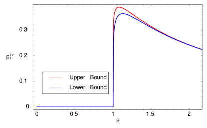
Figure 7: (Color online) Bounds for $p^{xz}_{n}$ obtained by imposing the positivity of the eigenvalues of the reduced density operator $\rho_{ij}$.

Since we have all the correlation functions at hand we proceed with the calculations of $G(1)$ and $G(2,i_{1})$. Remembering that for the Ising model $p^{y}=0$ Eq. (20) can be written as

$$G(1)=1-(p^{x})^{2}-(p^{z})^{2}.$$ (57)

As we have already shown $G(1)$ is the mean linear entropy of one spin which, due to translational symmetry, is equal to the linear entropy of any spin of the chain. A similar related analysis was done by Osborne and Nielsen nielsen for the von Neumann entropy instead of the linear entropy. As well as $G(1)$, see Fig. 9, the von Neumann entropy is maximal at the critical point nielsen . At that time Osborne and Nielsen did not give much importance to this result since they suspected that the von Neumann entropy of one spin with the rest of the chain does not measure genuine MES. However, for a translational symmetric state it is a reasonable good indication of genuine ME as we have shown in previous sections. (We have explicitly studied the linear entropy but the same results apply to the von Neumann entropy. We have adopted the former mainly due to its simplicity and relation to the Meyer and Wallach global entanglement meyer ).

Analyzing Eq. (57) we can understand why $G(1)$ is maximal at the critical point ($\lambda=1$). As we explain in what follows, it is $\langle\sigma^{x}\rangle$ the main responsible for this behavior of $G(1)$. For $\lambda\leq 1$ we have $\langle\sigma^{x}\rangle=0$. After the critical point, however, $\langle\sigma^{x}\rangle\neq 0$. Moreover, for $\lambda>1$ Eq. (54) tells us that $\langle\sigma^{x}\rangle$ is a monotonic increasing function of $\lambda$ and that $\langle\sigma^{x}\rangle\rightarrow 1$ as $\lambda\rightarrow\infty$. Therefore, since $\langle\sigma^{z}\rangle$ is negligible for large values of $\lambda$ and $\langle\sigma^{x}\rangle\approx 1$ (See Fig. 8) we must have $G(1)$ approaching zero after the critical point.

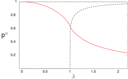
Figure 8: (Color online) Magnetizations $p^{x}$ $=$ $\langle\sigma^{x}\rangle$ (black/dashed line) and $p^{z}$ $=$ $\langle\sigma^{z}\rangle$ (red/solid line) as a function of $\lambda$.

We now analyze $G(2,i_{1})$. Using the Ising model symmetries Eq. (24) reads,

$$G(2,n)=1-\frac{1}{3}\left[2(p^{x})^{2}+2(p^{z})^{2}+2(p^{xz}_{n})^{2}+\right.$$

$$\left.(p^{xx}_{n})^{2}+(p^{yy}_{n})^{2}+(p^{zz}_{n})^{2}\right].$$ (58)

With Eq. (58) we can evaluate $G(2,n)$ for any value of $n$. In Fig. 9 we have plotted $G(1)$ and the bonds for $G(2,1)$. We can see that both $G(1)$ and $G(2,1)$ are maximum at the critical point $\lambda=1$. Notice that the bounds are very tight and can barely be distinguished just in a small region for $\lambda\gtrsim 1$. Furthermore, $G(2,1)$ is always smaller than $G(1)$, contrary to what was obtained using zero as a lower bound nossopaper . As well as in the case of $G(1)$ we can see that the reason for $G(2,1)$ being maximal at the critical point is due to the behavior of $\langle\sigma^{x}\rangle$ since it is the only function in Eq. (58) that does not change smoothly as we cross the critical point (see Fig. 10 for the other correlation functions).

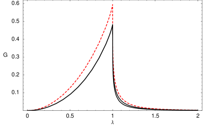
Figure 9: (Color online) G(1) (red/dashed line) and the bounds for G(2,1) (black/solid lines). Note that they are maximum at the critical point.

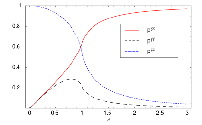
Figure 10: (Color online) Two point correlation functions: $p_{1}^{xx}$ (red/solid), $-p_{1}^{yy}$ (black/long-dashed), and $p_{1}^{zz}$ (blue/short-dashed).

We have also plotted $G(2,n)$ for $n=1$, $7$, and $15$ (Fig. 11). We can observe that all of them are maximum at the critical point and increase as a function of $n$ (In Fig. 11 we have plotted only the upper bounds since the lower bounds produce very similar curves). We also note that $G(2,7)$ is very near $G(2,15)$ showing that $G(2,n)$ rapidly saturates to a fixed value. At the critical point we have $\lim_{n\rightarrow\infty}G(2,n)=0.675$. This behavior for $G(2,n)$ points in the direction of the existence of multipartite entanglement at the critical point since any two spins are entangled with the rest of the chain and this entanglement increases with the distance between them. It is also interesting to confront this result with the fact that two spins that are separated by two or more sites are not entangled since their concurrences are zero Nature .

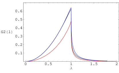
Figure 11: (Color online) $G(2,n)$ for $n=1,7$, and $15$. From bottom to top $n=1,7$, and $15$

The behavior of the concurrence ($C(n)$) can also be understood if we note that it can be expressed in terms of the one and two point correlation functions. While for the non-symmetric (ferromagnetic) state the analytical expression for the concurrence is cumbersome for the symmetric one it is very simple. Fortunately, for the Ising model it was show that the concurrence does not change upon symmetry break nome_dificil1 ; nome_dificil2 and it turns out to be

$$C(n)=\frac{1}{2}\left(-1-p_{n}^{yy}+p_{n}^{xx}+p_{n}^{zz}\right).$$ (59)

From this expression we can see that the concurrence (Fig. 12) does not depend on either the off-diagonal correlation function $p_{n}^{xz}$ or on the one point correlation functions (magnetizations). This is an interesting feature and helps us to understand why the concurrence is not maximum at the critical point.

Figure 12: Concurrence for nearest neighbors.

IV Conclusion

A $N$-partite quantum system may be entangled in many distinct ways. To characterize and to define a good measure of entanglement for those systems is a hard problem. The only simple alternative, valid whenever the joint $N$-system state is pure, is to split the system into two partitions and compute the entanglement in that way. This bipartition could be constructed in many different forms and thus give distinct amount of entanglement. One possible approach is to divide the system into two blocks of $L$ and $N-L$ subsystems and to compute the block entanglement latorre ; latorre2 between the two blocks. However one could think of a situation where all of the subsystems in the block $L$ are entangled with each other, as well as the subsystems of block $N-L$, but without any entanglement between the two blocks. For this situation the block entanglement would quantify a zero amount of entanglement, which is clearly not true. A valid bipartition approach, which would be able to quantify the entanglement in such a situation, is to compute the entanglement for all kinds of bipartition and then to average these to give the total amount of entanglement in the system.

In this article we have formalized an operational multipartite entanglement measure, the generalized global entanglement ($E_{G}^{(n)}$), firstly introduced in Ref. nossopaper . For $n=1$, $E_{G}^{(n)}$ recovers the Meyer and Wallach global entanglement measure meyer . However for $n>1$ $E_{G}^{(n)}$ together with the auxiliary function $G(n,i_{1},i_{2},\ldots,i_{n-1})$ quantify entanglement in the many distinct forms it is distributed in a multipartite system. We have shown that for some multipartite systems the original global entanglement is not able to properly classify and identify multipartite entanglement in a unequivocally way, whereas higher classes ($n>1$) of $E_{G}^{(n)}$ are. A genuine $k$-partite entangled state is the one that cannot be written as a product $|\phi\rangle_{l}\otimes|\psi\rangle_{(k-l)}$ of state vectors for any $l<k$, meaning that there is no other reduced pure state out of the joint $k$-systems state. To completely quantify and classify the multipartite entanglement in this kind of state one would have to compute all the $E_{G}^{(n)}$ classes up to $n=k-1$. However we have observed that lower classes of $E_{G}^{(n)}$, such as $E_{G}^{(1)}$ and $E_{G}^{(2)}$, are sufficient to detect multipartite entanglement. The computation of higher orders of $E_{G}^{(n)}$ and of the auxiliary functions $G(n,i_{1},i_{2},\ldots,i_{n-1})$ is necessarily required only to distinguish and classify the ways the system is entangled. Although the calculation of all those higher orders may be operationally laborious it is straightforward to perform for finite $N$ systems. Thus we have demonstrated for a variety of genuine multipartite entangled qubit states osterloh ; chua that $E^{(2)}_{G}$ and $G(2,i_{1})$ are able to properly identify and distinguish them whereas $E_{G}^{(1)}$ fails to do so. Inspired by the common characteristic presented by all $G(2,i_{1})$ for those paradigmatic states we then discussed an operational definition of a genuine multipartite entangled state osterloh ; chua .

Finite multipartite systems are interesting for fundamental discussions on the definition of multipartite entanglement. Infinite systems on the other hand are interesting since multipartite entanglement may be relevant to improve our knowledge of quantum phase transition processes occurring in the thermodynamical limit. We have demonstrated that for the 1D Ising model in a transverse magnetic field both $E_{G}^{(2)}$ and $G(2,i_{1})$ are maximal at the quantum critical point, suggesting thus a favorable picture for the occurrence of a genuine multipartite entangled state. Moreover, the behavior of $G(2,i_{1})$ and thus $E_{G}^{(2)}$ can be easily understood as contributions of the one and two-point correlation functions giving us a physical picture for the behavior of the multipartite entanglement during the phase transition process.

In conclusion the generalized global entanglement we presented has the following important features: (1) It is operationally easy to be computed, avoiding any minimization process over a set of quantum states; (2) It has a clear physical meaning, being for each class $E_{G}^{(n)}$ the averaged $n$-partition purity; (3) It is able to order distinct kinds of multipartite entangled states whereas other common measures fail to do so; (4) It is able to detect second order quantum phase transitions, being maximal at the critical point. (5) Finally, for two-level systems it is given in terms of correlation functions, and thus easily computed for a variety of available models. We hope that this measure may contribute for both the understanding of entanglement in multipartite systems and for the understanding of the relevance of entanglement in quantum phase transitions.

- (1) E. Schrödinger, Proc. Camb. Phil. Soc. 31, 555 (1935).
- (2) A. Einstein, B. Podolsky, and N. Rosen, Phys. Rev. 47, 777 (1935).
- (3) J. S. Bell, Physics 1, 195 (1964).
- (4) M. A. Nielsen and I. L. Chuang, Quantum Computation and Quantum Information (Cambridge University Press, Cambridge, 2000).
- (5) W. K. Wootters, Phys. Rev. Lett. 80, 2245 (1998).
- (6) S. L. Braunstein and P. van Loock, Rev. Mod. Phys. 77, 513 (2005).
- (7) W. Dür, G. Vidal, and J. I. Cirac, Phys. Rev. A 62, 062314 (2000).
- (8) F. Verstraete, J. Dehaene, B. De Moor, and H. Verschelde, Phys. Rev. A 65, 052112 (2002).
- (9) Richer classifications with more parameters can be pursued. For instance, we can have a multipartite state where four subsystems are entangled, another five are entangled, and the remaining subsystems are separable. We would need now two parameters to classify this state.
- (10) T. R. de Oliveira, G. Rigolin, and M. C. de Oliveira, Phys. Rev.A 73, 010305(R) (2006).
- (11) D. A. Meyer and N. R. Wallach, J. Math. Phys. 43, 4273 (2002).
- (12) H. Barnum, E. Knill, G. Ortiz, R. Somma, and L. Viola, Phys. Rev.Lett. 92, 107902 (2004).
- (13) R. Somma, G. Ortiz, H. Barnum, E. Knill, and L. Viola, Phys. Rev. A 70, 042311 (2004).
- (14) G. K. Brennen, Quantum Inf. Comp. 3, 619 (2003).
- (15) A. Lakshminarayan and V. Subrahmanyam, Phys. Rev. A 71, 062334 (2005).
- (16) J. I. Latorre, E. Rico, and G. Vidal, Quantum Inf. Comp. 4, 48 (2004) and references therein.
- (17) G. Vidal, J. I. Latorre, E. Rico, and A. Kitaev, Phys. Rev. Lett. 90, 227902 (2003).
- (18) We remark that A. J. Scott in Ref. scott has previously arrived to a simmilar generalization of the Meyer-Wallach global entanglement from a somewhat different approach. In our form however, due to the definition in terms of the auxiliary function , the many facets of the multipartite entanglement are clearly represented through the classes of .
- (19) A. J. Scott, Phys. Rev. A 69, 052330 (2004).
- (20) O. F. Syljuåsen, Phys. Rev. A 68, 060301(R) (2003).
- (21) O. F. Syljuåsen, eprint quant-ph/0312101.
- (22) D. M. Greenberger, M. A. Horne, A. Shimony, and A. Zeilinger, Am. J. Phys. 58, 1131 (1990).
- (23) G. Rigolin, Phys. Rev. A 71, 032303 (2005).
- (24) A. Osterloh and J. Siewert, Phys. Rev. A 72, 012337 (2005).
- (25) Y. Yeo and W. K. Chua, Phys. Rev. Lett. 96, 060502 (2006).
- (26) V. Coffman, J. Kundu, and W. K. Wootters, Phys. Rev. A 61, 052306 (2000).
- (27) C. P. Yang and G. C. Guo, Chin. Phys. Lett. 17, 162 (2000).
- (28) G. Vidal and R. F. Werner, Phys. Rev. A 65, 032314 (2002).
- (29) Another way of interpreting Definition 1 is to consider it as a sufficient condition for a state to be a genuine MES.
- (30) T. J. Osborne and M. A. Nielsen, Phys. Rev. A 66, 032110 (2002).
- (31) A. Osterloh, L. Amico, G. Falci and R. Fazio, Nature 416, 608 (2002).
- (32) S. Sachdev, Quantum Phase Transitions (Cambridge University Press, Cambridge, 1999).
- (33) P. Pfeuty, Ann. Physics (New York) 57, 79 (1970).
- (34) J. D. Johnson and B. M. McCoy, Phys. Rev. A 4, 2314 (1971).
- (35) T. Roscilde, P. Verrucchi, A. Fubini, S. Haas, and V. Tognetti, Phys. Rev. Lett. 94, 147208 (2005).
- (36) F. Verstraete, M. A. Martin-Delgado, and J. I. Cirac, Phys. Rev. Lett. 92, 087201 (2004).
- (37) L. Campos Venuti, C. Degli Esposti Boschi, M. Roncaglia, and A. Scaramucci, Phys. Rev. A 73, 010303(R) (2006).