Spatial Orientation using Quantum Telepathy

Abstract

We implemented the protocol of entanglement assisted orientation in the space proposed by Brukner et al. (quant-ph/0509123). We used min-max principle to evaluate the optimal entangled state and the optimal direction of polarization measurements which violate the classical bound.

Bizarre effects of quantum entanglement Schrodinger35 ,EPR35 , are usually dramatized using Bell’s inequalities Bell64 ,CHSH69 ,FC72 ,Tsirelson80 . These show that correlations between measurements on two spatially separated systems can be higher than anything allowed by the ”local realistic” (i.e. classical) theories. The way that testing Bell’s inequalities almost invariably proceeds is, in very broad terms, as follows. Alice and Bob share a number of entangled pairs, and Alice measures her systems at the same time as Bob measures his systems. After that, they communicated classically their results to each other and compute various correlation functions. When they combine these correlation functions into a Bell’s inequality, they can then check if the inequality is violated (signifying the existence of correlations stronger than any classical one). It is crucial for this experiment that Alice and Bob classically communicate with each other. Otherwise they would never be able to compute the necessary correlation functions in order to test the inequality. It is absolutely extraordinary, however, that there are applications where Alice and Bob could utilize stronger than classical correlations without any form of classical communication.

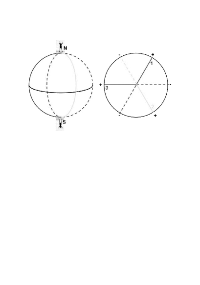
Figure 1: Two partners (Alice and Bob) are on the two poles of the Earth: there are three paths and two directions (+ and -) for each path: each partner have to find the other in the lack of any classical communication. To achieve their goal the best strategy is to maximize the probability to take the same directions, if they choose the same path, and the probability to take opposite directions if they choose different paths.

Suppose that Alice and Bob are far away from each other, but happen to share some entanglement (this could have been established when they met at some earlier time). Can they, using entanglement but without utilizing any classical communication, move in the direction towards each other faster than allowed by any local realistic theories? Namely can they find each other without communication? Surprisingly, this protocol is possible as shown very recently by Brukner et al in Brukner05 . The way that this would proceed is that, depending on the outcomes of their respective measurements, Alice and Bob would move in certain directions, and entanglement would ensure that the directions are such that they (on average) approach each other faster than allowed classically and yet without communicating with each other. This protocol clearly exemplifies why entanglement deserves to be called ”spooky”. The effect could, in fact, be called ”spatial orientation using quantum telepathy”.

In this letter we experimentally demonstrate that quantum entanglement indeed leads to the faster than classical orientation in space.

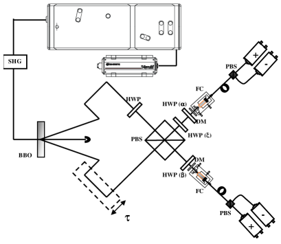
Figure 2: Experimental set-up. A 3 mm long $\beta$-barium borate crystal, cut for a Type.II phase-matching, is pumped in ultrafast regime.The SPDC photon pairs, are generated as coherent superposition of $\left|HV\right\rangle$ and $\left|VH\right\rangle$. The HWP changes the two alternatives in $\left|HH\right\rangle$ and $\left|VV\right\rangle$.The PBS provides the symmetrization of amplitude probabilities. The temporal superposition of the two alternatives is reached by changing the length of the trombone $\left(\tau\right)$. At the output of the interferometer the Bell state $\left|\Phi^{+}\right\rangle$ is synthesized. By tilting the BBO crystal and rotating the third HWP it is possible to synthesize all Bell States or a linear combinationof two of them KKCGS03 ,BCDC04 .

Two partners (Alice and Bob) are on the two poles of the Earth; there are three paths and two directions (+ and -) for each path: each partner have to find the other in the lack of any classical communication (Fig.1). To achieve their goal the best strategy is to maximize the probability to take the same directions, if they choose the same path, and the probability to take opposite directions if they choose different paths. The overall probability of success is given by

$$P=\frac{1}{9}\left(\sum\limits_{i=1}^{3}P_{ii}\left(same\right)+\sum\limits_{i\neq j=1}^{3}P_{ij}\left(opp\right)\right)$$ (1)

where $P_{ij}\left(opp\right)$ is the probability that Alice and Bob take opposite direction, if they choose different paths, $P_{ii}\left(same\right)$ is the probability that they take the same direction if they choose the same path.

The probability of success of any classical protocol is bounded by the value 7/9, because it was demonstrated that

$$\beta=\sum\limits_{i=1}^{3}P_{ii}\left(same\right)+\sum\limits_{i\neq j=1}^{3}P_{ij}\left(opp\right)\leq 7$$ (2)

holds for all local realistic models Brukner05 .

To increase the probability of success, Alice and Bob can share polarization-entangled photon pairs: every partner independently choose a path at random from the set {1,2,3}. The choice of the path determines a choice of direction of polarization measurements: the possible outputs (+ or -) fix the direction along the path.

The aim of this letter is to use the min-max principle to evaluate the optimal entangled state and the optimal direction of polarization measurements which violate the classical bound.

The min-max principle for self-adjoint transformations Halmos74 states that the operator norm is bounded by the minimal and maximal eigenvalues. The norm of the self-adjoint transformation resulting from the sum of the quantum counterparts of all the classical terms contributing to a particular Bell inequality obeys the min-max principle. Thus determining the maximal violations of classical Bell inequalities amounts to solving an eigenvalue problem. The associated eigenstates are the multi-partite states which yield a maximum violation of the classical bounds under the given experimental setup Werner01 ,Filipp04 ,Cabello04 .

In order to evaluate the quantum counterpart of the inequality (2), the classical probabilities have to be substituted by the quantum ones. Let us consider a two spin 1/2 particles configuration, described by its density matrix $\rho$, in which the two particles move in opposite directions along the y axis and the spin components are measured in the x-z plane. In such a case, the single particle spin-up and down observables along $\vartheta_{i}$, $\vartheta_{j}$, correspond to the projections $A_{\pm}\left(\vartheta_{i}\right)$, with

$$A_{\pm}\left(\vartheta\right)=\frac{1}{2}\left(\mathbf{I}\pm\mathbf{n}\left(\vartheta\right)\mathbf{\sigma}\right)$$ (3)

where $\mathbf{\sigma}$ is the vector of the Pauli matrices. The joint probability $q_{ij\text{ }}$for finding the left particle in the spin-up state along the angle $\vartheta_{i}$ and the right particle in the spin-up state along the angle $\vartheta_{j}$ is given by

$$q_{ij\text{ }}=tr\{\rho[A_{+}\left(\vartheta_{i}\right)\otimes A_{+}\left(\vartheta_{j}\right)]\}.$$ (4)

Then, substituting in the inequality (2), we obtain

$$P_{ii}\left(same\right) =tr\{\rho[A_{+}\left(\vartheta_{i}\right)\otimes A_{+}\left(\vartheta_{i}\right)$$

$$+A_{-}\left(\vartheta_{i}\right)\otimes A_{-}\left(\vartheta_{i}\right)]\},$$

$$P_{ij}\left(opp\right) =tr\{\rho[A_{+}\left(\vartheta_{i}\right)\otimes A_{-}\left(\vartheta_{j}\right)$$

$$+A_{-}\left(\vartheta_{i}\right)\otimes A_{+}\left(\vartheta_{j}\right)]\}.$$ (5)

We are interested in maximal violations of the inequality (2) with three possible measurements setting per observer: Alice and Bob choose between three dichotomic observables, determined by three measurements angles $\vartheta_{1}$, $\vartheta_{2}$, $\vartheta_{3}$.

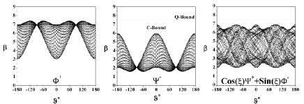
Figure 3: Experimentally reconstructed bounds for eigenvalues $\lambda_{1,2,3,4}\left(\varphi,\vartheta\right)$. The bounds for eigenvalues $\lambda_{3,4}\left(\varphi,\vartheta\right)$ were reached by the linear combination of the Bell states $\left|\Psi^{+}\right\rangle$ and $\left|\Phi^{-}\right\rangle$.

The first possible choice is given by $\vartheta_{1}=0$, $\vartheta_{2}=2\varphi$, $\vartheta_{3}=2\vartheta$. In this case the eigenvalues $\lambda_{1,2,3,4}$, and the eigenvectors $\nu_{1,2,3,4}$, corresponding to the maximal violating eigenstates of the self-adjoint operator $O_{33}$

$$O_{33} =\sum\limits_{s\in\{+,-\}}\sum\limits_{i=1}^{3}A_{s}\left(\vartheta_{i}\right)\otimes A_{s}\left(\vartheta_{i}\right)$$

$$+\sum\limits_{s\neq t\in\{+,-\}}\sum\limits_{i\neq j=1}^{3}A_{s}\left(\vartheta_{i}\right)\otimes A_{t}\left(\vartheta_{j}\right)$$ (6)

are

$$\lambda_{1}\left(\varphi,\vartheta\right) =6-\cos\left(2\vartheta\right)-\cos\left(2(\vartheta-\varphi)\right)-\cos\left(2\varphi\right)$$

$$\lambda_{2}\left(\varphi,\vartheta\right) =3+\cos\left(2\vartheta\right)+\cos\left(2(\vartheta-\varphi)\right)+\cos\left(2\varphi\right)$$

$$\lambda_{3}\left(\varphi,\vartheta\right) =\frac{1}{2}\left\{9-\left[15+2\cos\left(4\vartheta\right)-4\cos\left(2(\vartheta-2\varphi)\right)\right.\right.$$

$$-4\cos\left(2(2\vartheta-\varphi)\right)+2\cos\left(4(\vartheta-\varphi)\right)$$

$$\left.\left.+2\cos\left(4\varphi\right)-4\cos\left(2(\vartheta+\varphi)\right)\right]^{1/2}\right\}$$

$$\lambda_{4}\left(\varphi,\vartheta\right) =\frac{1}{2}\left\{9+\left[15+2\cos\left(4\vartheta\right)-4\cos\left(2(\vartheta-2\varphi)\right)\right.\right.$$

$$-4\cos\left(2(2\vartheta-\varphi)\right)+2\cos\left(4(\vartheta-\varphi)\right)$$

$$\left.\left.+2\cos\left(4\varphi\right)-4\cos\left(2(\vartheta+\varphi)\right)\right]^{1/2}\right\}$$ (7)

$$\nu_{1} =\left|\Phi^{+}\right\rangle$$

$$\nu_{2} =\left|\Psi^{-}\right\rangle$$

$$\nu_{3} =F\left(\varphi,\vartheta\right)\left|\Psi^{+}\right\rangle+G\left(\varphi,\vartheta\right)\left|\Phi^{-}\right\rangle$$

$$\nu_{4} =H\left(\varphi,\vartheta\right)\left|\Psi^{+}\right\rangle+I\left(\varphi,\vartheta\right)\left|\Phi^{-}\right\rangle$$ (8)

where the eigenvectors $\nu_{3}$ and $\nu_{4}$ are given by the superposition of the Bell’s states $\left|\Psi^{+}\right\rangle$, $\left|\Phi^{-}\right\rangle$, by the functions F, G, H, I. The maximum eigenvalue is $\lambda_{1}\left(\varphi,\vartheta\right)$ with the corresponding eigenvector $\left|\Phi^{+}\right\rangle$, and optimal angles of measurement given by $\left(60^{o},-60^{o}\right)$ (when we consider angles less than $90^{o}$), where is achieved the value 7.5. The second eigenvalue $\lambda_{2}\left(\varphi,\vartheta\right)$ with eigenvector $\left|\Psi^{-}\right\rangle$, determinates the minimum bound for the inequality (2). For the angles $\left(60^{o},-60^{o}\right)$, the minimum value 1.5 is reached. The eigenvalues $\lambda_{3}\left(\varphi,\vartheta\right)$ and $\lambda_{4}\left(\varphi,\vartheta\right)$ stay always under the classical bound $7$. For a single value parametrization, for example, $\vartheta_{1}=0$, $\vartheta_{2}=2\vartheta$, $\vartheta_{3}=-2\vartheta,$ the eigenvalues $\lambda_{1,2,3,4}$, and the eigenvectors $\nu_{1,2,3,4}$, corresponding to the maximal violating eigenstates of the self-adjoint operator $O_{33}$ are

$$\lambda_{1} =6-2\cos\left(2\vartheta\right)-\cos\left(4\vartheta\right)\text{, }\nu_{1}=\left|\Phi^{+}\right\rangle$$

$$\lambda_{2} =5+2\cos\left(2\vartheta\right)-\cos\left(4\vartheta\right)\text{, }\nu_{2}=\left|\Psi^{+}\right\rangle$$

$$\lambda_{3} =4-2\cos\left(2\vartheta\right)+\cos\left(4\vartheta\right)\text{, }\nu_{3}=\left|\Phi^{-}\right\rangle$$

$$\lambda_{4} =3+2\cos\left(2\vartheta\right)+\cos\left(4\vartheta\right)\text{, }\nu_{4}=\left|\Psi^{-}\right\rangle$$ (9)

then the entangled state $\left|\Phi^{+}\right\rangle$ provides the violation of classical bound for $\vartheta=60^{o}$. In this case to any eigenvalue one Bell state corresponds.

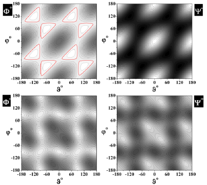
Figure 4: The contour plots represent the experimental reconstruction of $\beta$ for the bidimesional parametrization $\left(0,2\varphi,2\vartheta\right)$. Only the state $\left|\Phi^{+}\right\rangle$ violates the classical bound 7. For the states $\left|\Phi^{+}\right\rangle$ and $\left|\Psi^{-}\right\rangle$ the corresponding plots represents, also, the bidimensional eigenvalues $\lambda_{1,2}\left(\varphi,\vartheta\right)$, i.e., the maximum and the minimum bound of $O_{33}$. The state $\left|\Phi^{-}\right\rangle$ reaches the classical bound 7.

In the experimental set-up (see Fig.2), a 3 mm long $\beta$-barium borate crystal, cut for a TypeII phase-matching Klyshko88 , KMWZSS95 , Rubin96 , is pumped in ultrafast regime (120 fs) by a train of $\Omega_{\mathit{pump}}=410$ nm pulses generated by the second harmonic of a Ti:Sa laser. SPDC (Spontaneous Parametric Down-Converted) photon pairs at 820 nm $\left(\Omega_{\mathit{pump}}/2\right)$ are generated with an emission angle of $3^{o}$. After passing through the interferometer, thanks to temporal engineering and amplitude symmetrization, we obtain the entangled state

$$\left|\Phi^{+}\right\rangle=\frac{1}{\sqrt{2}}\left(\left|HH\right\rangle+\left|VV\right\rangle\right)$$ (10)

where H (V) stays for Horizontal (Vertical). The photons are coupled by lenses into single-mode fibers. Coupling efficiency has been optimized by a proper engineering of the pump and the collecting mode in experimental conditions BVCCDS03 . Dichroic mirrors are placed in front of the fiber couplers to reduce stray light due to pump scattering. Half Wave Plates (HWPs) before the fiber coupler, together with fiber-integrated polarizing beam splitters (PBSs), project photons in the polarization basis $\left|s\left(2\vartheta\right)\right\rangle=\cos\left(\vartheta\right)\left|H\right\rangle+\sin\left(\vartheta\right)\left|V\right\rangle$, $\left|s^{\bot}\left(2\vartheta\right)\right\rangle=\sin\left(\vartheta\right)\left|H\right\rangle-\cos\left(\vartheta\right)\left|V\right\rangle$. Photons are detected by single photon counters (Perkin-Elmer SPCM-AQR-14). A third HWP ($\xi$) provides to prepare the superposition of two Bell states ($\left|\Psi^{+}\right\rangle$ and $\left|\Phi^{-}\right\rangle$) to experimentally reconstruct all two-dimensional bounds BCDC04 .

The local observables $\hat{A}_{\pm}(\vartheta_{i})$ can be rewritten for the chosen polarization basis $\left\{\left|s(2\vartheta)\right\rangle,\left|s^{\bot}(2\vartheta)\right\rangle\right\}$ as

$$\hat{A}_{+} =|s(2\vartheta)\rangle\langle s(2\vartheta)|$$

$$\hat{A}_{-} =|s^{\bot}(2\vartheta)\rangle\langle s^{\bot}(2\vartheta)|$$ (11)

and the correlation functions (4) can be expressed in terms of coincidence detection probabilities $p_{x,y}\left(\vartheta_{i},\vartheta_{j}\right)$ as:

$$\left\langle A_{+}\left(\vartheta_{i}\right)\otimes A_{+}\left(\vartheta_{i}\right)+A_{-}\left(\vartheta_{i}\right)\otimes A_{-}\left(\vartheta_{i}\right)\right\rangle$$

$$=p_{++}\left(\vartheta_{i},\vartheta_{i}\right)+p_{--}\left(\vartheta_{i},\vartheta_{i}\right)$$ (12)

$$\left\langle A_{+}\left(\vartheta_{i}\right)\otimes A_{-}\left(\vartheta_{j}\right)+A_{-}\left(\vartheta_{i}\right)\otimes A_{+}\left(\vartheta_{j}\right)\right\rangle$$

$$=p_{+-}\left(\vartheta_{i},\vartheta_{j}\right)+p_{-+}\left(\vartheta_{i},\vartheta_{j}\right)$$ (13)

where $x,y=+,-$ are the two outputs of the integrated PBS and $p_{x,y}\left(\vartheta_{i},\vartheta_{j}\right)$ are expressed in terms of coincident counts:

$$p_{x,y}\left(\vartheta_{i},\vartheta_{j}\right)=\frac{N_{x,y}\left(\vartheta_{i},\vartheta_{j}\right)}{N_{TOT}}$$ (14)

where $N_{x,y}\left(\vartheta_{i},\vartheta_{j}\right)$ is the number of coincidences measured by the pair of detectors $x,y$ in the above described polarization basis, and $N_{TOT}=N_{++}\left(\vartheta_{i},\vartheta_{j}\right)+N_{+-}\left(\vartheta_{i},\vartheta_{j}\right)+N_{-+}\left(\vartheta_{i},\vartheta_{j}\right)+N_{--}\left(\vartheta_{i},\vartheta_{j}\right)$.

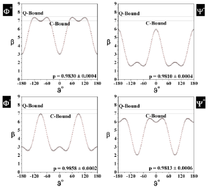
Figure 5: Experimental reconstruction of $\beta$ for parametrization $\left(0,2\vartheta,-2\vartheta\right)$. A non-ideal state affected by white noise can be written as: $p\left|\Phi^{+}\right\rangle\left\langle\Phi^{+}\right|+\frac{\left(1-p\right)}{4}I.$ The maximum experimental value is $\beta\simeq 7.41$ and from the corresponding fit function we obtained the value $p\simeq 0.98$.

In Fig.3 we show the experimentally reconstructed bounds for eigenvalues $\lambda_{1,2,3,4}\left(\varphi,\vartheta\right)$. The bounds for eigenvalues $\lambda_{3,4}\left(\varphi,\vartheta\right)$ are reached by the linear combination of the Bell states $\left|\Psi^{+}\right\rangle$ and $\left|\Phi^{-}\right\rangle$. In addition, in Fig.4 we show the contour plots representing the experimental reconstruction of the Bell operator $\beta$ for the bi-dimensional parametrization $\left(0,2\varphi,2\vartheta\right)$: only the state $\left|\Phi^{+}\right\rangle$ violates the classical bound $7$. For the states $\left|\Phi^{+}\right\rangle$ and $\left|\Psi^{-}\right\rangle$ the corresponding plots represents, also, the bi-dimensional eigenvalues $\lambda_{1,2}\left(\varphi,\vartheta\right)$, i.e., the maximum and the minimum bound of $O_{33}$. The state $\left|\Phi^{-}\right\rangle$ reaches the classical bound $7$. In Fig.5 we show the experimental reconstruction of $\beta$ for the mono-dimensional parametrization $\left(0,2\vartheta,-2\vartheta\right)$, and, in particular, the violation of the maximum values of the Bell operator $\beta$ for the state $\left|\Phi^{+}\right\rangle.$ Due to the experimental imperfections (misalignment and presence of stray light), the state generated from the source could be written as $p\left|\Phi^{+}\right\rangle\left\langle\Phi^{+}\right|+\frac{\left(1-p\right)}{4}I$, including a white noise term: from the experimental value $\beta\simeq 7.41$ and the corresponding fit function, we obtained $p\simeq 0.98$.

Thus it could seem not surprising that a maximally entangled state is the one violating classical forecasts and providing a ”speed-up” in spatial orientation, the actual demonstration of this conclusion is not obvious and could be not valid for different Bell’s like inequalities. Moreover, the fact that the $\left|\Phi^{+}\right\rangle$ state, and only this maximally entangled state, violates the inequality (2) is undoubtedly not a priori predictable. In this context the min-max principle definitely appears as a powerful tool.

These experiments were carried out in the Quantum Optics Labs at Elsag spa, Genova, within EC-FET project QAP-2005-015848. The authors thank Caslav Brukner for helpful discussions.

References

(1)E. Schrödinger,
Proc. Cambridge Philos. Soc. 31, 555 (1935).
(2)A. Einstein, B. Podolsky, and N. Rosen,
Phys. Rev. 47, 777 (1935).
(3)J.S. Bell,
Physics (Long Island City, N.Y.) 1, 195 (1964).
(4)J.F. Clauser, M.A. Horne, A. Shimony, and R.A. Holt,
Phys. Rev. Lett. 23, 880 (1969).
(5)S.J. Freedman and J.F. Clauser,
Phys. Rev. Lett. 28, 938 (1972); E.S. Fry and R.C. Thompson,
Phys. Rev. Lett. 37, 465 (1976);
A. Aspect, J. Dalibard, and G. Roger,
Phys. Rev. Lett. 49, 1804 (1982).
(6)B.S. Cirel’son [Tsirelson],
Lett. Math. Phys. 4, 93 (1980).
(7)C. Brukner, N. Paunkovic, T. Rudolph, V. Vedral
quant-ph/0509123
(8)P.R. Halmos, Finite-dimensional vector spaces
(Springer, New York, Heidelberg, Berlin, 1974); M. Reed and B. Simon,
Methods of Modern Mathematical Physics IV: Analysis of Operators
(Academic Press, New York, 1978).
(9)R.F. Werner and M.M. Wolf, Phys. Rev. A 64, 032112 (2001);
(10)S. Filipp and K. Svozil, Phys. Rev A 69, 032101
(2004); S. Filipp and K. Svozil, Phys. Rev. Lett. 93, 130407 (2004).
(11)A. Cabello, Phys. Rev. Lett. 92, 060403 (2004).
(12)D.N. Klyshko, Photons and Nonlinear Optics (Gordon
and Breach, New York, 1988).
(13)P.G. Kwiat, K. Mattle, H. Weinfurter, A. Zeilinger,
A.V. Sergienko, and Y. Shih,
Phys. Rev. Lett. 75, 4337 (1995).
(14)M.H. Rubin,
Phys. Rev. A 54, 5349 (1996).
(15)Y.-H. Kim, S.P. Kulik, M.V. Chekhova, W.P. Grice, and
Y. Shih,
Phys. Rev. A 67, 010301(R) (2003).
(16)F.A. Bovino, G. Castagnoli, I.P. Degiovanni, and
S. Castelletto,
Phys. Rev. Lett. 92, 060404 (2004).
(17)F.A. Bovino, P. Varisco, A.M. Colla, G. Castagnoli,
G. Di Giuseppe, and A.V. Sergienko, Opt. Comm. 227, 343 (2003).