Electromagnetic manipulation for anti-Zeno effect
in an engineered quantum tunneling process

Abstract

We investigate an anti-Zeno phenomenon as well as a quantum Zeno effect for the irreversible quantum tunneling from a quantum dot to a ring array of quantum dots. By modeling the total system with the Anderson-Fano-Lee model, it is found that the transition from the quantum Zeno effect to quantum anti-Zeno effect can happen by adjusting magnetic flux and gate voltage.

I Introduction

The modern development of quantum technology enables people to control quantum process of microscopic system by external field Lloyd ; Scull ; zanar ; sun-xue ; kuri1 ; kuri2 . In the point of view of quantum mechanics, the objective of a quantum control is to reach a desired state (called target state) from an initial state of the controlled system by manipulating its external parameters. Some aspects in quantum information can be understood according to quantum control Qc-qc . For example, quantum computation, which manipulates the evolution of a quantum system by appropriate logic gate operations, is essentially a quantum control process by external parameters. In quantum error correction, the feedback control is used to detect the unwanted couplings and correct them Lloyd . Quantum measurement can also be regard as a special control process, which projects the unknown state into the definite state that we desired with maximized probability through wave function collapse.

In quantum control, an intriguing conception is to use the quantum Zeno effectSudar ; Misra . Such effect freezes the evolution of a quantum state through frequent measurements. For instance, in the quantum bang-bang controlLloyd , the measurement operations are generalized by a sequence of pulses. Recently a quantum control scheme associated with the effect opposite to the quantum Zeno effect was discovered, which accelerate the decay of the unstable state by frequent measurements. Such effect is called anti-Zeno effect (AZE) Kurizki1 ; Lewens ; Kurizki5 ; Levit ; Kurizki7 or inverse Zeno effect. This discovery opens a new area for quantum control and has been used to control various physical systems, such as trapped atoms in an optical-lattice potential Raizen , a superconducting current-biased Josephson junction Kurizki4 , ultracold atomic condensates Kurizki6 , and etc.

In this paper, we consider the anti-Zeno effect with an engineered system formed by an experimentally accessible ring-type quantum dot array and an extra quantum dot. Here, the extra dot is coupled with one of dot array. Since it is an artificial system with more flexibly controlled parameters, we can study the dynamic detail of the transition between quantum Zeno effect and quantum anti-Zeno effect in the one-direction quantum tunneling of electron from the extra dot to the quantum dot array. Our main purpose is to find a way controlling the electron tunneling. Our investigation is mainly based on the discovery that the $k$-space representation of the quantum dot ring model is equivalent to the famous Anderson-Fano-Lee model fano ; ander ; Lee , which correctly describes the irreversible quantum process of a single energy level coupling with a continuous-spectra bath. Then the standard approach luisell is used to obtain the analytic solution for the quantum tunneling dynamics. We also consider the tunneling dynamics of bosons in a one-dimensional optical lattice with the same configuration as that of fermions.

This paper is organized as follows: In section II, we describe the engineered model of quantum dot array. Then we point out that its $k$-space representation is essentially the Anderson-Fano-Lee model. In section III, we study the quantum irreversible process of quantum tunneling in the Heisenberg picture. In section IV, we calculate the modified tunneling rate by successive projective measurements, which are performed on one dot to detect whether an electron is trapped here. We also recur to a numerical calculation to confirm our observation. In section V, we discuss the similar problems for bosons. Finally in section VI, we conclude the paper with some remarks.

II Quantum dot array model for one-direction quantum tunneling

We begin with a system of $2N$ identical quantum dots arranged in a ring threaded by a magnetic flux $\phi$. Here, each structureless quantum dot only traps one electron in a single state. The sites of the quantum dot ring are labeled by $0,1$ $\cdots$ $2N-1$. The $0$th quantum dot interacts with an additional quantum dot beside those placed on the ring, as is illustrated schematically in Fig. 1(a).

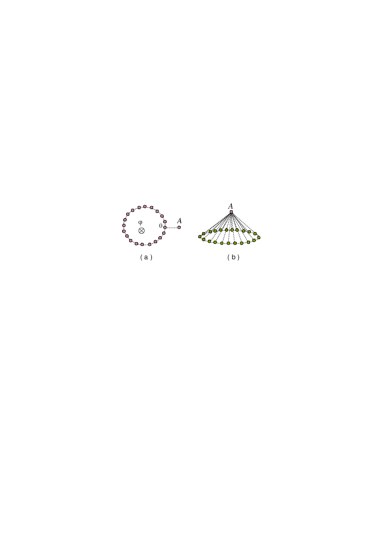
Figure 1: (Color on line) (a)The real space schematic illustration for 2N identical quantum dots arranged in a ring threaded by a magnetic flux, with 0th dot interacting with dot $A$. (b) The virtual space schematic illustration for a ring quantum dot array coupled with quantum dot $A$ homogeneously.

Under the tight-binding approximation, the model Hamiltonian reads Peier ; suncp2 ; Koski ; Fath

$$H = \hbar J\sum_{j=0}^{2N-1}e^{i\frac{\pi}{N}\phi}\hat{a}_{j}^{\dagger}\hat{a}_{j+1}$$

$$+\hbar\omega_{A}\hat{a}_{A}^{\dagger}\hat{a}_{A}+\hbar g\hat{a}_{0}^{\dagger}\hat{a}_{A}+H.c.,$$

which describes the electron tunneling dynamics of this quantum dots system controlled by a magnetic flux. Here, $J$ denotes the hopping integral over the $j$th site and the $j+1$th site. For simplicity, we assume $J$ is a constant. $g$ is the coupling strength between two quantum dots at the $0$th site and the additional site $A$; $\omega_{A}$ is the on-site potential (or called the chemical potential) of $A$ site; $\phi$ is the magnetic flux through the ring, and $a_{j}^{{\dagger}}$($a_{j}$) is the fermion creation (annihilation) operator at the $j$th site. We note here that the above Hamiltonian was presented by Peierls Peier to study the magnetic flux effect phenomenologically up to the second order approximation.

We consider a dual picture (Fig.1b) of the above quantum dot model illustrated by Fig.1(a). Through the Fourier transformation

$$\hat{a}_{j}=\frac{1}{\sqrt{2N}}\sum_{k=0}^{2N-1}e^{i\frac{\pi}{N}kj}\hat{a}_{k},$$ (2)

the original Hamiltonian is transformed into a $k$-space representationlieb . In this momentum representation, the Hamiltonian becomes

$$H = \hbar\sum_{k=0}^{2N-1}\epsilon_{k}\hat{a}_{k}^{\dagger}\hat{a}_{k}+\hbar\omega_{A}\hat{a}_{A}^{\dagger}\hat{a}_{A}$$

$$+\frac{\hbar g}{\sqrt{2N}}\sum_{k=0}^{2N-1}\left(\hat{a}_{k}^{\dagger}\hat{a}_{A}+h.c.\right),$$

where

$$\epsilon_{k}=2J\cos\frac{\pi}{N}\left(\phi+k\right)$$ (4)

is the well-known Bloch dispersion relation. In this dual model (II), the quantum dots in a ring type array are coupled to the single quantum dot $A$ homogeneously. The $2N$ modes of the ring quantum dot array are characterized by the operators $\hat{a}_{k}^{\dagger}$s and $\hat{a}_{k}$s, which create and annihilate a quasi-excitation in the $k$th mode.

From the above dual picture of the quantum dot array model, it can be observed that a one-direction quantum tunneling in our quantum dot model can occur as a typical quantum dissipation phenomenon. Since the quantum dot $A$ is coupled to other quantum dots of the ring array, the electron in this dot can easily tunnel into the array, but it is very difficult for all the electrons in the array to go back to the dot $A$ simultaneously. Thus the electron in the quantum dot $A$ will experience an irreversible process. This similar phenomenon was studied as the Fano model fano for atom physics, the Anderson model for condensed matter physics ander and even as the Lee model for particle physics Lee . In this paper we focus on the quantum control problem for the irreversible quantum tunneling, namely, we explore the possibility of changing the microscopic quantum tunneling process by adjusting the external fields, since many parameters in such an artificially engineered system can be tuned to a great extent.

III Evolution dynamics in Heisenberg picture

The total system described by Hamiltonian (II) is isolated as a closed system, but the electron in each dot, such as dot $A$, is an open system. When the dynamics of the system we are interested is only the quantum dot $A$, the quantum dot array can be regarded as an engineered environment. In terminology of quantum open system approach, the Hamiltonian (II) describes a single level system interacting with an environment suncp1 . Such an engineered environment is composed of an ensemble of $2N$ qubits. State $|1\rangle$ denotes one electron in the dot, and $|0\rangle$ denotes no electron in the dot. The unitary operator generated by the Hamiltonian (II) entangles the system with the environment.

Now we investigate dynamics of the model (II) in the Heisenberg picture. The Heisenberg equation driven by the Hamiltonian (II) results in the following equations

$$\frac{d}{dt}\hat{a}_{k}\left(t\right)=-i\epsilon_{k}\hat{a}_{k}-\frac{ig}{\sqrt{2N}}\hat{a}_{A},$$ (5)

$$\frac{d}{dt}\hat{a}_{A}\left(t\right)=-i\omega_{A}\hat{a}_{A}-ig\sum_{k=0}^{2N-1}\frac{\hat{a}_{k}}{\sqrt{2N}}.$$ (6)

The motions of $\hat{a}_{k}$ and $\hat{a}_{A}$ are coupled via the coupling constant $g$. For the convenience in the following discussions, we only consider its short-time behavior, by employing the operator ordering prescription. We should point out that the short-time behavior has been studied in RefKurizki1 for the general case with the coupling of a discrete state to a continuum. With an analytical approach in Schrödinger picture, they found that the decay processes of the single state coupling to a discrete or a continuous spectrum is determined by the energy spread incurred by the measurementsKurizki1 . Our approach will be carried out in the Heisenberg picture for the present realistic system.

Defining two new fermion operators

$$\hat{C}_{k}=\hat{a}_{k}e^{i\epsilon_{k}t},\hat{B}=\hat{a}_{A}e^{i\omega_{A}t},$$ (7)

to remove the high frequency effect, we have the integral-differential equation as

$$\frac{d\hat{B}}{dt} = -\frac{ig}{\sqrt{2N}}\sum_{k=0}^{2N-1}e^{-i\left(\epsilon_{k}-\omega_{A}\right)t}\hat{C}_{k}\left(0\right)$$ (8)

$$-\frac{g^{2}}{2N}\sum_{k=0}^{2N-1}\int_{0}^{t}\hat{B}\left(t_{1}\right)e^{i\left(\epsilon_{k}-\omega_{A}\right)(t_{1}-t)}dt_{1}$$

from the above Eqs.(5) and (6). Integrating both sides of Eq.(8), we proceed with an iteration method to obtain the suitable operator ordering prescription for the dynamic evolution of $\hat{a}_{k}\left(t\right)$ and $\hat{a}_{A}\left(t\right)$. If the coupling strength $g$ is small, we can omit the terms with the order of $g$ higher than two. It is a reasonable assumption that $\hat{a}_{A}\left(t\right)$ varies slowly within a short time interval. By replacing $\hat{B}\left(t_{1}\right)$ with $\hat{B}\left(0\right)$ in the right hand side of the above equation, the evolution of annihilation operator $\hat{a}_{A}\left(t\right)$ is approximately calculated as

$$\hat{a}_{A}\left(t\right) = \hat{a}_{A}\left(0\right)e^{-i\omega_{A}t}-$$

$$\sum_{k=0}^{2N-1}\frac{ig\hat{a}_{k}\left(0\right)}{\sqrt{2N}}e^{-i\omega_{A}t}\int_{0}^{t}e^{-i\left(\epsilon_{k}-\omega_{A}\right)t^{\prime}}dt^{\prime}$$

$$-\hat{a}_{A}\left(0\right)e^{-i\omega_{A}t}\int_{0}^{t}dt^{\prime}\left(t-t^{\prime}\right)e^{i\omega_{A}t^{\prime}}\Phi\left(-t^{\prime}\right),$$

where the memory function Kurizki4

$$\Phi\left(t\right)=\frac{g^{2}}{2N}\sum_{k=0}^{2N-1}e^{i\epsilon_{k}t},$$ (10)

only depends on the quasi-excitation in the $2N$ modes of the ring quantum dot array and the magnetic flux.

IV Quantum tunneling affected by a sequence of projective measurements

Now we consider the decay of tunneling rate induced by an instantaneous projective measurement into the initial state of the total system. Suppose that the entire system is initially prepared in a state with an electron in the quantum dot $A$ and no electron in the ring array. Let $\left|0\right\rangle$ denotes the vacuum state that no electron exists in the entire system. Then, the initial state can be written as

$$\left|\psi\left(0\right)\right\rangle=\hat{a}_{A}^{\dagger}\left(0\right)\left|0\right\rangle.$$ (11)

Obviously, this state is unstable since the electron may tunnel to any dot of the quantum dot array in Fig.1(b). After a period of evolution, the probability for finding the electron inside the dot $A$ and no electrons in the ring array is

$$p\left(t\right)=\left|\left\langle\psi\left(0\right)\right|U\left(t\right)\left|\psi\left(0\right)\right\rangle\right|^{2},$$ (12)

where $U\left(t\right)=\exp\left(-iHt/\hbar\right)$ is the unitary operator.

Assume the coupling strength $g$ is small. For a projective measurement into the initial state, the probability for finding the electron in the initial state is

$$p\left(t\right)=\exp\left(-Rt\right),$$ (13)

which decays exponentially with a decay rate $R$ calculated as

$$R=2\text{Re}\int_{0}^{t}dt^{\prime}G(t,t^{\prime})e^{-i\omega_{A}t^{\prime}}\Phi\left(-t^{\prime}\right),$$ (14)

where $\Phi\left(t^{\prime}\right)$ is just the memory function we defined above and $\ G(t,t^{\prime})=\left(1-t^{\prime}/t\right)$. It has the similar expression to what obtained in Refs.Kurizki1 ; Lewens ; Kurizki5 ; Levit ; Kurizki7 .

To justify the above result, we assume the system is initially prepared in $\left|\psi\left(0\right)\right\rangle=\hat{a}_{A}^{\dagger}\left(0\right)\left|0\right\rangle$. The probability for finding the electron inside the dot $A$ and no electrons in the array is $p\left(t\right)=\left|\left\langle 0\right|\hat{a}_{A}\left(t\right)\left|1_{A}\right\rangle\right|^{2}$. With the explicit expression Eq.(III) for $\hat{a}_{A}\left(t\right)$, we obtain

$$p\left(t\right)=\left|1-\int_{0}^{t}dt^{\prime}\left(t-t^{\prime}\right)e^{-i\omega_{A}t^{\prime}}\Phi\left(-t^{\prime}\right)\right|^{2}.$$ (15)

Since $g$ is small and $\Phi\left(t\right)$ is proportional to $g^{2}$, we approximately have

$$p\left(t\right)\approx\left|e^{-\int_{0}^{t}dt^{\prime}\left(t-t^{\prime}\right)e^{-i\omega_{A}t^{\prime}}\Phi\left(-t^{\prime}\right)}\right|^{2}$$ (16)

or Eq.(13) with $R(t)$ defined by Eq.(14).

After such measurements have been done by $n=t/\tau$ times, the survival probability for finding the electron still in dot $A$ is

$$p\left(t=n\tau\right) = e^{-2n\int_{0}^{\tau}dt^{\prime}\left(\tau-t^{\prime}\right)e^{-i\omega_{A}t^{\prime}}\Phi\left(-t^{\prime}\right)}$$

$$= e^{-2t\int_{0}^{\tau}dt^{\prime}G(\tau,t^{\prime})e^{-i\omega_{A}t^{\prime}}\Phi\left(-t^{\prime}\right)}$$

$$= e^{-2t\text{Re}\int_{0}^{+\infty}dt^{\prime}G(\tau,t^{\prime})\Theta\left(\tau-t^{\prime}\right)e^{-i\omega_{A}t^{\prime}}\Phi\left(-t^{\prime}\right)},$$

which gives the decay rate modified by measurement

$$R=2\text{Re}\int_{0}^{+\infty}dt^{\prime}G(\tau,t^{\prime})\Theta\left(\tau-t^{\prime}\right)e^{-i\omega_{A}t^{\prime}}\Phi\left(-t^{\prime}\right),$$ (18)

where $\Theta\left(x\right)$ is the Heaviside unit step function, i.e. $\Theta\left(x\right)=1$ for $x>0$, and $\Theta\left(x\right)=0$ for $x<0$.

Define the modulation function caused by measurement as

$$f\left(t\right)=G(\tau,t)e^{-i\omega_{A}t}\Theta\left(\tau-t\right).$$ (19)

By applying the Fourier transformation to the modulation function $f\left(t\right)$ and the memory function $\Phi\left(-t\right)$, the decay rate modified by the projective frequently measurement is calculated as

$$R=\frac{g^{2}\tau}{4\pi N}\sum_{m=0}^{2N-1}sinc^{2}\left[\left(J\cos\frac{\left(\phi+m\right)\pi}{N}-\frac{\omega_{A}}{2}\right)\tau\right].$$ (20)

Eq.(20) shows that the decay rate $R$ depends on four parameters: the time interval $\tau$ between two successive measurements; the number $2N$ of quantum dots placed on the ring; the on-site-potential $\omega_{A}$ which is applied to the dot $A$ by the electrode; and the magnetic flux $\phi$ through the ring quantum dot array, but only $\tau$, $\omega_{A}$ and $\phi$ can be adjusted experimentally.

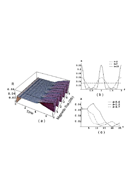
Figure 2: (Color on line)(a) 3-D diagram for the behavior of the decay rate as a function of $\tau$ and $\phi$ under the setting $J=5,g=1,N=20$ and $\omega_{A}=0$. (b) The cross sections of the 3-D surface for $\tau=2,7,15$. (c)The cross sections of the 3-D surface for $\phi=0.6,1.2,2.7$. It shows the tunneling rate can be modulated by the magnetic flux. The unit of time interval is $\hbar$ and the unit of magnetic flux is Wb.

To study the dynamic details of the irreversible quantum tunneling, we first consider the dynamic behavior of electron with no measurement performed. Fermi golden rule is used to calculate the decay rate as

$$R=\frac{g^{2}}{4N}\sum_{m=0}^{2N-1}\delta\left(2J\cos\frac{\left(\phi+m\right)\pi}{N}-\omega_{A}\right).$$ (21)

Eq.(21) shows the decay rate depends on $\omega_{A}$, $N$ and $\phi$. If $\left|\omega_{A}\right|\leq 2J$ and the number of quantum dots placed on the ring is finite, two situations happen to the electron motion when one adjusts the magnetic flux $\phi$: 1) The electron tunnels into the quantum dot array arranged in the ring and never come back; 2) the electron stays in site $A$. In the following, we will explain the physical mechanism for the switch between these two situations by adjusting $\phi$: the energy level of the ring quantum dot array is discrete in Fig.1(b), and the electron tunneling between dots occurs when the discrete energy level of one dot matches that of the other dot. The magnetic flux $\phi$ controls the discrete energy levels of the quantum dot array to match or not to match the energy level of quantum dot $A$ so that the above two phenomenon occur. As the number of quantum dots placed on the ring increases, the discrete energy levels of the dot array approach with each other. Thus the effect of magnetic flux $\phi$ becomes vanishing, and the controllable parameter is only the on-site potential $\omega_{A}$. The two phenomena described above happen to the electron when $\left|\omega_{A}\right|$ is smaller or larger than $2J$.

Actually, as for Eq.(21), one can also use the Wigner-Weisskopf approach luisell to describe the electron dynamic evolution approximately. To this end, we first take the Laplace transformation of Eq.(8)

$$\hat{B}\left(s\right)=\frac{\hat{B}\left(0\right)}{f\left(s\right)}-\sum_{k=0}^{2N-1}\frac{ig\hat{C}_{k}\left(0\right)}{\sqrt{2N}f\left(s\right)\left[s+i\left(\epsilon_{k}-\omega_{a}\right)\right]}\text{,}$$ (22)

where

$$f\left(s\right)=s+\sum_{k=0}^{2N-1}\frac{g^{2}/\left(2N\right)}{s+i\left(\epsilon_{k}-\omega_{a}\right)}.$$ (23)

As the coupling strength $g$ is small, the Wigner-Weisskopf approach gives the zero point of $f\left(s\right)$ luisell , which results in the approximate solution

$$\hat{B}\left(t\right)=\hat{B}\left(0\right)e^{-Rt}-\sum_{k=0}^{2N-1}\frac{ige^{-Rt}\hat{C}_{k}\left(0\right)}{\sqrt{2N}[i\left(\epsilon_{k}-\omega_{A}\right)-R]}\text{,}$$ (24)

where $R$ has the same expression as Eq.(21). So long as the Wigner-Weisskopf approximation is valid for some time interval, the above solution can correctly describe the quantum tunneling phenomenon in the coupling quantum dot configuration.

Next we study the dynamic behavior of electron in quantum tunneling when $\tau\rightarrow 0$, i.e. the system is measured continuously. In this case the decay rate for the electron tunneling from quantum dot $A$ to the quantum dot array vanishes. This means the electron is frozen in the quantum dot $A$.

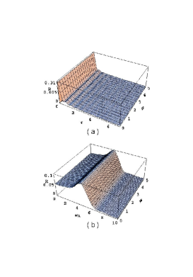
Figure 3: (Color on line) The independence of the decay rate $R$ on magnetic flux $\phi$. (a) 3-D diagram for the behavior of the decay rate as a function of $\tau$ and $\phi$ under the setting $J=5,g=1,N=20$ and $\omega_{A}=20$. (b) 3-D diagram for the behavior of the decay rate as a function of $\omega_{A}$ and $\phi$ under the setting $J=2.5,g=1,N=20$ and $\tau=10$.

Then we consider the behavior of the electronic quantum tunneling with the finite time interval between two successive measurements. Due to the finiteness of time interval, we find that only quantum anti-Zeno effect can occur in some cases. From Eq.(20), we can see when one of the energy levels of the ring dot array matches that of dot $A$, that is, the parameters $\phi$ and $\omega_{A}$ satisfy the following equation

$$2J\cos\frac{\left(\phi+m\right)\pi}{N}=\omega_{A}\text{,}$$ (25)

the tunneling rate is an increasing function of time interval $\tau$. Consequently, the quantum Zeno effect occurs. When all energy levels of the array are out of resonance with that of dot $A$, i.e. Eq.(25) can not be satisfied for any $m$, the tunneling rate is roughly a descending function of $\tau$. Thus the quantum anti-Zeno effect occurs. Hence, when the time interval $\tau$ between two successive measurements is finite, in the region of $|\omega_{A}|<2J$, the occurrence of quantum Zeno or anti-Zeno effect depends on the magnetic flux $\phi$ for a given on-site potential $\omega_{A}$; and for a given magnetic flux $\phi$, the occurrence of quantum Zeno or anti-Zeno effect depends on on-site potential $\omega_{A}$. In the region of $|\omega_{A}|>2J$, only quantum anti-Zeno effect occurs when the time interval $\tau$ is in a finite appropriate range.

In Fig.2 and Fig.3(a), we numerically plot the decay rate as the function of $\tau$ and the magnetic flux $\phi$ for different on-site potential $\omega_{A}$. Fig.2 is plotted when the on-site potential $\omega_{A}$ is just within the energy range of the ring dot array. It shows that, when the time interval approaching zero, the quantum Zeno effect does occur, which coincides with our above discussion; for a small time interval, the tunneling rate is a constant; for a appropriate time interval, whether the electron tunnels out of the quantum dot $A$ to other dot or stays in quantum dot $A$ is dependent on the magnetic flux. This means we can inhibit or accelerate the dissipative motion of the electron. Fig.3(a) shows that when the on-site potential $\omega_{A}$ is outside of the energy range $\left[-2J,2J\right]$, the tunneling rate only depends on the interval $\tau$. As $\tau\rightarrow 0$, the quantum Zeno effect also occurs, but there exists a range of a finite $\tau$, in this range, the system decays rapidly as the measurement frequency increases, so only the quantum anti-Zeno effect occurs. These verify our above arguments.

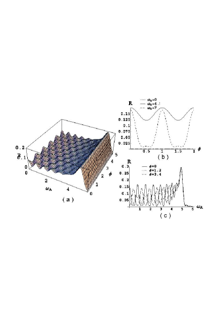
Figure 4: (Color on line)(a) 3-D diagram for the behavior of the decay rate as a function of $\omega_{A}$ and $\phi$ under the setting $J=2.5,g=1,N=20$ and $\tau=10$. (b) The cross sections of the 3-D surface for $\omega_{A}=0,4.5,7$. (c) The cross sections of the 3-D surface for $\phi=0,1.2,3.4$. It shows that the motion of the electron can be modulated by electromagnetism.

For different time interval $\tau$ between two successive measurements, in Fig.3(b) and Fig.4, we numerically plot the tunneling rate as the function of the magnetic flux $\phi$ and on-site potential $\omega_{A}$. In this system, $\omega_{A}$ is controlled by the electrochemical gate electrode. It can be seen that for sufficient small interval $\tau$, shown in Fig.3(b), the tunneling rate modified by measurement is independent of the magnetic flux $\phi$, but for an appropriate interval $\tau$, shown in Fig.4, one can modulate the tunneling rate by the magnetic flux when the on-site potential $\omega_{A}$ is smaller then $2J$.

V Irreversible quantum tunneling of boson in optical lattice

We consider the bosonic atoms trapped in a ring optical latticeCatali ; Wang , which is described as a periodic potential $V\left(x\right)=V\left(x+a\right)$ with spatial period $a$. In general, we can use the many-body Hamiltonian

$$H = \int\Psi^{{\dagger}}\left(x\right)\left[\frac{p^{2}}{2m}+V\left(x\right)\right]\Psi\left(x\right)$$

$$+\int dxdy\Psi^{{\dagger}}\left(x\right)\Psi^{{\dagger}}\left(y\right)W\left(x,y\right)\Psi\left(x\right)\Psi\left(y\right)$$

to describe quantum dynamics of many-atom system. In the case of dilute atomic gas, we can neglect the interaction term. When each potential well in the optical lattice is deep sufficiently, the tight-binding approximation can be used by assuming the wave function as $\Psi\left(x\right)=\sum_{j}b_{j}u_{j}\left(x\right)$, where $u_{j}\left(x\right)$ is localized around the site $j$. If we neglect the overlaps of two localized basis states which are not next-neighbor, the coefficient $b_{j}$ will be approximately described as a boson operator. Hence the Hamiltonian of such boson system Zolle ; Porto ; Bhat ; knight ; Martin can be approximated as Eq.(II) with $\phi=0$

$$H = \hbar J\sum_{j=0}^{2N-1}\hat{b}_{j}^{\dagger}\hat{b}_{j+1}+\hbar\omega_{A}\hat{b}_{A}^{\dagger}\hat{b}_{A}$$

$$+\hbar g\hat{b}_{0}^{\dagger}\hat{b}_{A}+H.c\text{.}$$

Here, $\hat{b}_{j}^{{\dagger}}$($\hat{b}_{j}$) is the creation (annihilation) operator of bosonic atoms and they satisfy the commutation relations.

By the Fourier transformation for the boson operators $\hat{b}_{j}^{{\dagger}}$ and $\hat{b}_{j}$, the boson model (V) can be transformed into a dual model similar to that of fermions (see the Eq.II)

$$H = \sum_{k=0}^{2N-1}\varepsilon_{k}\hat{b}_{k}^{{\dagger}}\hat{b}_{k}+\hbar\omega_{A}\hat{b}_{A}^{{\dagger}}\hat{b}_{A}$$

$$+\frac{g}{\sqrt{2N}}\sum_{k=0}^{2N-1}\left(\hat{b}_{k}^{\dagger}\hat{b}_{A}+\hat{b}_{A}^{\dagger}\hat{b}_{k}\right),$$

where the Bloch dispersion relation is $\varepsilon_{k}=2J\cos\left(\pi k/N\right)$.

We now use the Heisenberg equation to study the system dynamics. By considering the short-time behavior which is described in section III, we find the evolution of annihilation operator $\hat{b}_{A}$ is similar to Eq.(III)

$$\hat{b}_{A}\left(t\right) = \hat{b}_{A}\left(0\right)e^{-i\omega_{A}t}-$$

$$\sum_{k=0}^{2N-1}\frac{ig\hat{b}_{k}\left(0\right)}{\sqrt{2N}}e^{-i\omega_{A}t}\int_{0}^{t}e^{-i\left(\varepsilon_{k}-\omega_{A}\right)t^{\prime}}dt^{\prime}$$

$$-\hat{b}_{A}\left(0\right)e^{-i\omega_{A}t}\int_{0}^{t}dt^{\prime}\left(t-t^{\prime}\right)e^{i\omega_{A}t^{\prime}}\Psi\left(-t^{\prime}\right),$$

where

$$\Psi\left(t\right)=\frac{g^{2}}{2N}\sum_{k=0}^{2N-1}e^{i\varepsilon_{k}t}$$ (30)

is the memory functionKurizki4 . Thus we can consider the decay of atomic tunneling rate modified by an instantaneous projective measurement with respect to the initial state of the total system. Unlike fermions, there can be more than one boson in a site. Thus, in the following we will investigate the decay rate of this system with respect to three different initial states, and try to find the behavior difference between boson and fermion.

First suppose the total system is initially prepared in a Fock state $\hat{b}_{A}^{\dagger}|0\rangle$ with only one atom in lattice site $A$. By $M$ successive instantaneous projective measurements into $\hat{b}_{A}^{\dagger}|0\rangle$, the decay rate is of the form

$$\Gamma=\frac{g^{2}\tau}{4\pi N}\sum_{m=0}^{2N-1}sinc^{2}\left[\left(J\cos\frac{m\pi}{N}-\frac{\omega_{A}}{2}\right)\tau\right]\text{,}$$ (31)

which is exactly the fermion tunneling rate with magnetic flux $\phi=0$. It can be seen from Eq.(31) that the atomic tunneling rate only depends on three parameters: the time interval $\tau$ between two successive measurements, the number of lattice sites arranged on the ring, and the on-site potential $\omega_{A}$ which is controlled by the laser intensity, but only $\tau$ and $\omega_{A}$ can be adjusted experimentally. When $\tau$ is very small and approaches zero, the well-known quantum Zeno effect occurs, and the system’s evolution is frozen. For a finite number of sites, when $\tau$ has a finite value, the quantum Zeno effect and anti-Zeno effect can be switched by adjusting the laser intensity: the quantum Zeno effect occurs when controllable variable $\omega_{A}=2J\cos\left(m\pi/N\right)$, and the anti-Zeno effect occurs when on-site potential $\omega_{A}\neq 2J\cos\left(m\pi/N\right)$ or $\left|\omega_{A}\right|>2\left|J\right|$. Also for a finite number of sites, when no measurement is performed, the system decays rapidly and the atom never goes back to site $A$ when $\omega_{A}=2J\cos\left(m\pi/N\right)$ for arbitrary $m$; when $\omega_{A}\neq 2J\cos\left(m\pi/N\right)$ or $\left|\omega_{A}\right|>2\left|J\right|$, the system never evolved and the atom stay in site $A$ for ever. When the number of sites $2N\rightarrow\infty$, the energy of the ring array become continuous, and thus for a proper $\tau$, the switch between quantum Zeno and anti-Zeno effect is determined by whether $\left|\omega_{A}\right|$ is larger or smaller than $2\left|J\right|$.

Now we consider the case with one site containing particles more than one. Assume the initial state of this total system is a number state $\left|n_{A}\right\rangle$ with all $n$ particles in site $A$. After time $t$, the probability for finding $\left|n_{A}\right\rangle$ is

$$p\left(t\right)=\frac{1}{n!}\left|\left\langle 0\right|\left[\hat{b}_{A}\left(t\right)\right]^{n}\left|n_{A}\right\rangle\right|^{2}\text{.}$$ (32)

By substituting Eq.(V) into Eq.(32), we find that after $M$ successive projective measurements into the initial state, the probability modified by the measurements has the similar form to Eq.(16)

$$p\left(t\right)=\exp\left[-2nt\int_{0}^{t}dt^{\prime}G(\tau,t^{\prime})e^{-i\omega_{A}t^{\prime}}\Psi\left(-t^{\prime}\right)\right]\text{.}$$ (33)

Through defining the modulation function introduced in Eq.(19), in the energy spectra, we find the atomic tunneling rate is $n$ times lager than that of fermion

$$\Gamma=n\frac{g^{2}\tau}{4\pi N}\sum_{m=0}^{2N-1}sinc^{2}\left(J\cos\frac{m\pi}{N}-\frac{\omega_{A}}{2}\right)\tau\text{.}$$ (34)

The value of Eq.(34) is demanded by four external controllable parameters: the time interval $\tau$, the number of sites placed on the ring, the on-site potential $\omega_{A}$ and the total number $n$ of atoms in the entire system. The new controllable element $n$ is added due to the boson enhancement effect. When $n$ is large, the bosonic atoms have a strong trend to leave site $A$. This just exhibits quantum statistic effect in quantum measurement for the localization of boson system.

Except for the $n$ enhancing decay of the boson atomic tunneling, the situation we discussed above is not surprising since they are very similar to that of fermion. To show the special features of the boson tunneling control, we consider the case with the initial state of this total system prepared in a quasi-classical state - the coherent state $|\alpha_{A}\rangle=D_{A}(\alpha)|0\rangle$, where

$$D_{A}(\alpha)=e^{{\alpha\hat{b}_{A}^{\dagger}-\alpha^{\ast}\hat{b}_{A}}}$$ (35)

is the displace operator. Like the Fock state listed above, this coherent state is also unstable, and the atoms at site $A$ may tunnel to the array. Once atoms are found in one site of the array, they will spread on the array by resonant tunneling. Thus, it is difficult for all the atoms to go back to site $A$. In order to keep all the atoms in their original state, a sequence of measurements are performed, which project the entire system into $|\alpha_{A}\rangle$. A measurement projects the system into the original state with probability

$$p\left(t\right)=\left|e^{-\left|\alpha\right|^{2}/2}\left\langle 0\right|e^{\alpha^{\ast}\hat{b}_{A}\left(t\right)}\left|\alpha\right\rangle\right|^{2}.$$ (36)

To calculate the explicit expression of the above probability, we define

$$r\equiv\int_{0}^{t}dt^{\prime}\left(1-\frac{t^{\prime}}{t}\right)e^{-i\omega_{A}t^{\prime}}\Psi\left(-t^{\prime}\right).$$ (37)

As the evolution of $\hat{b}_{A}\left(t\right)$ is already obtained in Eq.(V), we obtain the explicitly expression of probability

$$p\left(t\right) = e^{-\left|\alpha\right|^{2}\left(\left|\eta\left(t\right)\right|^{2}+3-4\cos\left(\omega_{A}\tau\right)\eta\left(t\right)\right)}\times$$ (38)

$$\exp\left[-\sum_{m}\frac{\left|\alpha g\right|^{2}\sin^{2}[\left(\varepsilon_{m}-\omega_{A}\right)\frac{t}{2}]}{N\left(\varepsilon_{m}-\omega_{A}\right)^{2}}\right],$$

where $\eta\left(t\right)=1-rt$. After $M$ successive projective measurements, we find the atomic tunneling rate $\Gamma$ is modified as

$$\Gamma=\frac{\left|\alpha\right|^{2}}{\tau}\left[\left|\eta\left(t\right)\right|^{2}+3-2\cos\left(\omega_{A}\tau\right)\eta\left(t\right)-\pi r\tau^{2}\right].$$ (39)

Here the expression of $r$ is transformed into the following form through Fourier transformation

$$r=\frac{g^{2}\tau}{4\pi N}\sum_{m=0}^{2N-1}sinc^{2}\left[J\cos\frac{m\pi}{N}-\frac{\omega_{A}}{2}\right]\tau.$$ (40)

In order to study the physical phenomena with $|\alpha_{A}\rangle$ as the initial state,

.

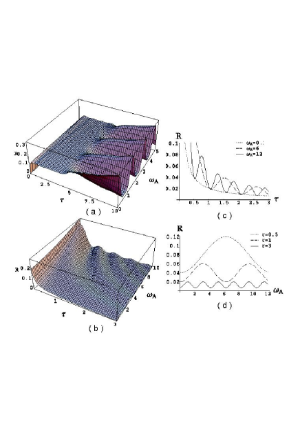
Figure 5: (Color on line) The behavior of the decay rate as a function of $\tau$ and $\omega_{A}$ with the system initial in a coherent state. (a) 3-D diagram for Fermi system with $J=5,g=2,N=20,\phi=0$. (b) 3-D diagram for Boson system with $J=5,g=0.01,N=20,\alpha=0.1$. (c) The cross sections of the 3-D surface for $\omega_{A}=0.1,6,12$. (d)The cross sections of the 3-D surface for $\tau=0.5,1,3$. It shows the tunneling rate can be slightly modulated by the intensity of laser beam, but in the gross, $\Gamma$ is a decreasing function of $\tau$ for any $\omega_{A}$.

in Fig.5, we numerically plot the decay rate as a function of two controllable external parameters $\tau$ and $\omega_{A}$. It shows that: 1) For a given on-site potential $\omega_{A}$, as $\tau\rightarrow 0$, this unstable state decays rapidly. This phenomenon is totally different from the fermion case, where the electron is frozen in its initial state. 2) For any on-site potential $\omega_{A}$, the tunneling rate can be slightly modulated by the intensity of laser beam, but in the gross, it is enhanced as the measurement frequency $1/\tau$ increasing. However in fermi system, the crossover of quantum Zeno and anti-Zeno effect can be controlled only by modulation of on-site potential.

VI Summary

In conclusion, we have investigated the quantum tunneling dynamics for both fermion and boson systems in an experimentally accessible engineered configuration respectively. In the case with electrons, the tunneling rate modified by the projective measurements can be controlled by the time interval between two successive measurements, the electrochemical gate electrode and the magnetic flux. Our results show that: 1) whatever the value of on-site potential $\omega_{A}$ is, for vanishing time interval, the quantum Zeno effect happens; 2) for $\omega_{A}$ off resonance with the energy of the dot array, the quantum anti-Zeno effect occurs as the measurement frequency increases; 3) for the on-site potential $\omega_{A}$ resonating the energy of the dot array, we can inhibit or accelerate the evolution of the electron by adjusting the magnetic flux and the on-site potential. In the case of boson system, generally, the time interval and the laser intensity control the decay of the system. The boson system shows an enhanced decay for quantum tunneling.

This work is supported by the NSFC with grant Nos. 90203018, 10474104 and 60433050, and NFRPC with Nos. 2001CB309310 and 2005CB724508. One (LZ) of the authors also acknowledges the support of K. C. Wong Education Foundation, Hong Kong.

References

- (1) L. Viola and S. Lloyd, Phys. Rev. A 58, 2733 (1998); S. Lloyd, Phys. Rev. A 62, 022108 (2000);
- (2) G. S. Agarwal, M.O. Scully, and H.Walther, Phys. Rev. A 63, 044101 (2001); Phys. Rev. Lett. 86, 4271 (2001).
- (3) P. Zanardi and S. Lloyd, Phys. Rev. A 69, 022313 (2004).
- (4) Fei Xue, S. X. Yu, and C. P. Sun , Phys. Rev. A 73 , 013403 (2006).
- (5) A. G. Kofman and G. Kurizki, Phys. Rev. Lett. 93, 130406 (2004).
- (6) S. Pellegrin and G. Kurizki, Phys. Rev. A 71, 032328 (2005).
- (7) V. Ramakrishna and H. Rabitz, Phys. Rev. A 54, 1715(1996).
- (8) B. Misra and E. C. G. Sudarshan, J. Math. Phys. 18, 756 (1977).
- (9) C. B. Chiu, E. C. G. Sudarshan, and B. Misra, Phys. Rev. D 16, 520 (1977).
- (10) A. G. Kofman and G. Kurizki, Nature (London ) 405, 546 (2000).
- (11) M. Lewenstein and K. Rza̧żewski, Phys. Rev. A 61, 022105 (2000).
- (12) A. G. Kofman and G. Kurizki, Phys. Rev. Lett. 87, 270405 (2001).
- (13) W. C. Schieve, L. P. Horwitz, and J. Levitan, Phys. Lett. A 136, 264 (1989).
- (14) A. G. Kofman and G. Kurizki, Phys. Rev. A 54, R3750 (1996).
- (15) M. C. Fischer, B. Gutierrez-Medina, and M. G. Raizen, Phys. Rev. Lett. 87, 040402 (2001).
- (16) A. Barone, G. Kurizki, and A. G. Kofman, Phys. Rev. Lett. 92, 200403 (2004).
- (17) I. E. Mazets, G. Kurizki,1 N. Katz, and N. Davidson, Phys. Rev. Lett. 94, 1907403 (2005).
- (18) U. Fano, Phys. Rev. 124, 1866 (1961).
- (19) P. W. Anderson, Phys. Rev. 124, 41 (1961).
- (20) T. D. Lee, Phys. Rev. 95, 1329 (1954).
- (21) W.H. Louisell, Quantum Statistical Properties of Radiation, (Wiley, New York, 1973)‘
- (22) R. Peierls, Z. Physik 80, 763 (1933).
- (23) S. Yang, Z. Song, C. P. Sun, Phys. Rev. A 73, 022317 (2006).
- (24) P. Koskinen and M. Manninen, Phys. Rev. B 68, 195304 (2003).
- (25) G. Fáth, J. Sólyom, Phys. Rev. B 47, 872 (1993).
- (26) Elliott Lieb, Theodore Schultz and Daniel Mattis, Ann. Phys. 16, 407 (1961).
- (27) C. P. Sun, H. Zhan, X. F. Liu, Phys. Rev. A 58, 1810 (1998).
- (28) L. Amico, A. Osterloh, and F. Cataliotti, Phys. Rev. Lett. 95, 063201 (2005).
- (29) X. Wang, Z. Chen, and P. G. Kevrekidis, Phys. Rev. Lett. 96, 083904 (2005).
- (30) D. Jaksch, C. Bruder, J. I. Cirac, C. W. Gardiner, and P. Zoller, Phys. Rev. Lett. 81, 3108 (1998).
- (31) Ana Maria Rey, Guido Pupillo, and J. V. Porto, Phys. Rev. A 73, 023608 (2006).
- (32) R. Bhat, M. J. Holland, and L. D. Carr, Phys. Rev. Lett. 96, 060405 (2006).
- (33) Jiannis K. Pachos and Peter L. Knight, Phys. Rev. Lett. 91, 107902 (2003).
- (34) André Eckardt, Christoph Weiss, and Martin Holthaus, Phys. Rev. Lett. 95, 260404 (2005).