Two-mode optical state truncation and generation of maximally entangled states in pumped nonlinear couplers

Abstract

Schemes for optical-state truncation of two cavity modes are analyzed. The systems, referred to as the nonlinear quantum scissors devices, comprise two coupled nonlinear oscillators (Kerr nonlinear coupler) with one or two of them pumped by external classical fields. It is shown that the quantum evolution of the pumped couplers can be closed in a two-qubit Hilbert space spanned by vacuum and single-photon states only. Thus, the pumped couplers can behave as a two-qubit system. Analysis of time evolution of the quantum entanglement shows that Bell states can be generated. A possible implementation of the couplers is suggested in a pumped double-ring cavity with resonantly enhanced Kerr nonlinearities in an electromagnetically-induced transparency scheme. The fragility of the generated states and their entanglement due to the standard dissipation and phase damping are discussed by numerically solving two types of master equations.

1 Introduction

Methods for preparation and manipulation of nonclassical states of light have become an important research area in quantum optics state , especially in relation to possible optical implementations of quantum computers and systems for quantum communication and quantum cryptography Nie00 . Among various schemes for optical-qubit generation, the so-called quantum scissors device of Pegg et al. Peg98 produces a superposition of vacuum and single-photon states, $c_{0}|0\rangle+c_{1}|1\rangle$, by optical-state truncation of an input single-mode coherent light. The Pegg et al. quantum scissors device was studied in numerous papers (see, e.g., Vil99 ; Kon00 ; Par00 ; Ozd01 ; Villas01 ; Mir04 ; Mir05 ), and tested experimentally by Babichev et al. Bab02 and Resch et al. Res02 . This simple scheme and its generalizations for truncation of an input optical state to a superposition of $d$ Fock states (the so-called qudits) Villas01 ; Mir05 are based on linear optical elements, and thus referred to as the linear quantum scissors devices. Optical-state ‘truncation’ can also be achieved in systems comprising nonlinear elements (e.g., Kerr media) Leo97 ; Dar00 , and thus will be referred to as the nonlinear quantum scissors devices. The above-mentioned schemes are restricted to the single-mode optical truncation. Here, by generalizing our former scheme Leo04 , we present a realization of nonlinear quantum scissors for optical-state truncation of two cavity modes by means of a pumped nonlinear coupler.

Two-mode nonlinear couplers have become, shortly after their introduction by Jensen Jen82 and Maier Mai82 , one of the important topics of photonics due to their wide potential applications and relative simplicity (see, e.g., reviews Sny91 ; Per00 ). Among various types of the nonlinear optical couplers, those based on Kerr effect have attracted especial interest both in classical Jen82 ; Mai82 ; Sny91 ; Gry01 and quantum Che96 ; Hor89 ; Kor96 ; Fiu99 ; Ibr00 ; Ari00 ; San03 ; ElOrany05 regimes. The Kerr nonlinear couplers can exhibit variations of self-trapping, self-modulation and self-switching effects. In quantum regime, they can also generate sub-Poissonian and squeezed light Hor89 ; Kor96 ; Fiu99 ; Ibr00 ; Ari00 . Possibilities of entanglement generation were also studied in nonlinear couplers operating by means of the Kerr effect San03 ; ElOrany05 or degenerate parametric down-conversion Her03 .

Here, we analyze Kerr nonlinear couplers, which can be modelled by systems composed of two quantum nonlinear oscillators linearly coupled to each other and placed inside a double-ring cavity. We discuss two schemes based on the coupler with an external excitation of a single mode and the coupler with two modes pumped. We show that the states generated in the excited nonlinear couplers under suitable conditions can be limited to a superposition of only vacuum and single-photon states, $c_{00}|00\rangle+c_{01}|01\rangle+c_{10}|10\rangle+c_{11}|11\rangle$. We compare the possibilities of generation of maximally entangled states by the couplers excited in single and two modes. We also discuss effects of dissipation on the fidelity of truncation and suggest a method to achieve strong Kerr interactions at low intensities in our system.

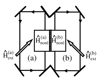
Figure 1: A realization of the two-mode nonlinear quantum scissors device via a pumped nonlinear coupler in a double-ring cavity. Symbols are explained in the text.

2 Coupler pumped in a single mode

We consider a system, referred to as the pumped Kerr nonlinear coupler, which consists of two nonlinear oscillators, with Kerr nonlinearities $\chi_{a}$ and $\chi_{b}$, linearly coupled to each other and additionally linearly coupled to an external classical field. In this section, we assume that the field is coupled to one of the oscillators only. Thus, the system can be described by the following Hamiltonian Leo04 ($\hbar=1$):

$$\hat{H} = \hat{H}_{0}+\hat{H}_{1},$$

$$\hat{H}_{0} = \omega_{a}\hat{a}^{\dagger}\hat{a}+\omega_{b}\hat{b}^{\dagger}\hat{b},$$

$$\hat{H}_{1} = \hat{H}^{(a)}_{\rm nonl}+\hat{H}^{(b)}_{\rm nonl}+\hat{H}_{\rm int}+\hat{H}^{(a)}_{\rm ext},$$ (1)

where

$$\hat{H}^{(a)}_{\rm nonl}+\hat{H}^{(b)}_{\rm nonl} = \frac{\chi_{a}}{2}(\hat{a}^{\dagger})^{2}\hat{a}^{2}+\frac{\chi_{b}}{2}(\hat{b}^{\dagger})^{2}\hat{b}^{2},$$ (2)

$$\hat{H}_{\rm int} = \epsilon\hat{a}^{\dagger}\hat{b}+\epsilon^{*}\hat{a}\hat{b}^{\dagger},$$ (3)

$$\hat{H}^{(a)}_{\rm ext} = \alpha\hat{a}^{\dagger}+\alpha^{*}\hat{a},$$ (4)

and $\hat{a}$ ($\hat{b}$) is the bosonic annihilation operator corresponding to the mode $a$ ($b$) of frequency $\omega_{a}$ ($\omega_{b}$). Hamiltonian (1) for $\hat{H}^{(a)}_{\rm ext}=0$ describes the standard nonlinear coupler Che96 ; Hor89 ; Kor96 ; Fiu99 ; Ibr00 ; Ari00 ; San03 ; ElOrany05 composed of two Kerr nonlinear oscillators linearly coupled to each other, where the parameter $\epsilon$ is the strength of this coupling. However, our model differs from the standard by inclusion of the extra term $\hat{H}^{(a)}_{\rm ext}$, which describes linear coupling between the driving single-mode classical field (say, with frequency $\omega_{\rm ext}^{(a)}$) and the cavity mode $a$. The parameter $\alpha$ describes the strength of this coupling and is proportional to the classical field amplitude. A possible physical realization of the model is presented in figure 1, where an external pump, described by $\hat{H}^{(b)}_{\rm ext}$, is off in the present analysis. Kerr media, marked by $\hat{H}^{(a)}_{\rm nonl}$ and $\hat{H}^{(b)}_{\rm nonl}$, are linearly coupled as described by grey central region corresponding to $\hat{H}_{\rm int}$.

The evolution of our system in the interaction picture can be described by the Schrödinger equation

$$i\frac{d}{dt}|\psi(t)\rangle=\hat{H}_{1}|\psi(t)\rangle,$$ (5)

where

$$|\psi(t)\rangle=\sum_{m,n=0}^{\infty}c_{mn}(t)|mn\rangle.$$ (6)

Thus, the complex probability amplitudes $c_{mn}(t)$ satisfy the set of equations of motion:

$$i\frac{d}{dt}c_{mn}=\left[\chi_{a}m(m-1)+\chi_{b}n(n-1)\right]c_{mn}$$

$$+\epsilon c_{m-1,n+1}\sqrt{m(n+1)}+\epsilon^{\ast}c_{m+1,n-1}\sqrt{(m+1)n}$$

$$+\alpha c_{m-1,n}\sqrt{m}+\alpha^{\ast}c_{m+1,n}\sqrt{m+1}.$$ (7)

A superficial analysis of (7) could lead to a conclusion that the evolution of the system pumped by classical external field cannot be restricted to two lowest photon-numer states, but will also include states with a greater number of photons. However, by generalizing the method of single-mode nonlinear quantum scissors proposed in Leo97 (for a review see MLI01 ; LM01 ), we have observed in Leo04 that evolution can be restricted to the only four states: $|00\rangle$, $|10\rangle$, $|01\rangle$ and $|11\rangle$ as a result of degeneracy of Hamiltonians $\hat{H}^{(a)}_{\rm nonl}$ and $\hat{H}^{(b)}_{\rm nonl}$. By assuming that the couplings $|\alpha|$, and $|\epsilon|$ are much smaller than the Kerr nonlinearities $\chi_{a}$ and $\chi_{b}$, we can interpret the evolution between the four states as resonant transitions, while the negligible evolution to other states as out of resonance, analogously to the single-mode case LM01 . This phenomenon can be shown explicitly as follows: under the assumption of $\chi_{a},\chi_{b}\gg\max(|\epsilon|,|\alpha|)$ and short evolution times, equation (7) for $m,n\neq 0,1$ can be approximated by

$$i\frac{d}{dt}c_{mn}\approx\left[\chi_{a}m(m-1)+\chi_{b}n(n-1)\right]c_{mn}$$ (8)

which has the simple solution

$$c_{mn}(t)\approx\exp\{-i\left[\chi_{a}m(m-1)+\chi_{b}n(n-1)\right]t\}c_{mn}(0).$$ (9)

By setting the initial condition $c_{mn}(0)=0$ for $m,n\neq 0,1$, one gets $c_{mn}(t)\approx 0$. By contrast, for $m,n\in\{0,1\}$, the terms proportional to $\chi_{a}$ and $\chi_{b}$ are vanishing due to degeneracy of the Kerr Hamiltonian and so the remaining terms proportional to $\epsilon$ and $\alpha$ are significant. Thus, the ideally ‘truncated’ two-mode state generated in the system has the following simple form

$$|\psi(t)\rangle_{\rm cut}=c_{00}(t)|00\rangle+c_{01}(t)|01\rangle+c_{10}(t)|10\rangle+c_{11}(t)|11\rangle,$$ (10)

where the evolution of $c_{mn}$, precisely given by (7), can approximately be described by the following equations

$$i\frac{d}{dt}c_{00} = \alpha^{*}c_{10},\quad i{\frac{d}{dt}}c_{01}\;=\;\epsilon^{*}c_{10}+\alpha^{*}c_{11},$$

$$i\frac{d}{dt}c_{11} = \alpha\,c_{01},\quad\;i\frac{d}{dt}c_{10}\;=\;\epsilon\,c_{01}+\alpha\,c_{00}.$$ (11)

Hereafter, in equations for the probability amplitudes under the discussed assumptions, sign ‘=’ should be understood as ‘$\approx$’. Although approximate equations (11) are independent of $\chi_{a}$, our derivation clearly shows that the Kerr nonlinearity plays a crucial role in the truncation process. By assuming that both oscillators are initially in vacuum states, $|\psi(t=0)\rangle=|00\rangle$, and parameters $\alpha$ and $\epsilon$ are real, we find the following solutions of (11) for the time-dependent probability amplitudes:

$$c_{00} = \frac{1}{2\gamma}\left[(\gamma-\epsilon)\cos\tau_{1}+(\gamma+\epsilon)\cos\tau_{2}\right],$$

$$c_{01} = \frac{\alpha}{\gamma}\left(\cos\tau_{1}-\cos\tau_{2}\right),$$

$$c_{10} = -\frac{i(\gamma+\epsilon)\Omega_{2}}{4\alpha\gamma}(\sin\tau_{1}+\sin\tau_{2}),$$

$$c_{11} = -\frac{i}{2\gamma}\left(\Omega_{2}\sin\tau_{1}-\Omega_{1}\sin\tau_{2}\right),$$ (12)

where $\Omega_{j}=\sqrt{2[2\alpha^{2}+\epsilon^{2}+(-1)^{j-1}\epsilon\gamma]}$, $\gamma=\sqrt{4\alpha^{2}+\epsilon^{2}}$, and $\tau_{j}=\Omega_{j}t/2$ for $j=1,2$. Note that the solution for $c_{10}$ can be written in a more symmetric form since the properties hold: $(\gamma+\epsilon)\Omega_{2}=(\gamma-\epsilon)\Omega_{1}=2\sqrt{\alpha^{2}(\gamma^{2}-\epsilon^{2})}$. In a special case of equal couplings $\alpha$ and $\epsilon$, (12) simplifies to our former solution Leo04 :

$$c_{00} = \cos(\sqrt{5}\tau)\cos(\tau)+\frac{1}{\sqrt{5}}\sin(\sqrt{5}\tau)\sin(\tau),$$

$$c_{01} = -\frac{2}{\sqrt{5}}\sin(\sqrt{5}\tau)\sin(\tau),$$

$$c_{10} = -i\frac{2}{\sqrt{5}}\sin(\sqrt{5}\tau)\cos(\tau),$$ (13)

$$c_{11} = -i\cos(\sqrt{5}\tau)\sin(\tau)+\frac{i}{\sqrt{5}}\sin(\sqrt{5}\tau)\cos(\tau),$$

where $\tau=\alpha t/2$. To estimate the quality of the optical-state truncation (up to single-photon states) of the generated light, we apply fidelity as a measure of discrepancy between the ideally truncated two-qubit state $\hat{\rho}_{\rm cut}=|\psi(t)\rangle_{\rm cut}\,{}_{\rm cut}\langle\psi(t)|$, given by (10), and the actually generated output state $\hat{\rho}(t)=|\psi(t)\rangle\langle\psi(t)|$ calculated numerically from

$$|\psi(t)\rangle=\exp(-i\hat{H}t)|00\rangle$$ (14)

for a large (practically infinite-dimensional) two-mode Hilbert space. Specifically, in our numerical analysis, we have chosen the dimension equal to $20$ for each subspace associated with single mode of the field. The fidelity, also referred to as the Uhlmann’s transition probability for mixed states, is defined by (see, e.g., Ved02 ):

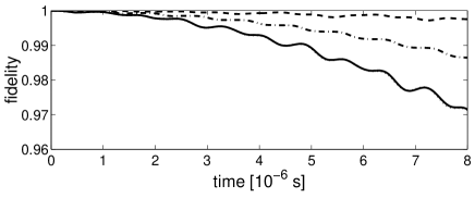
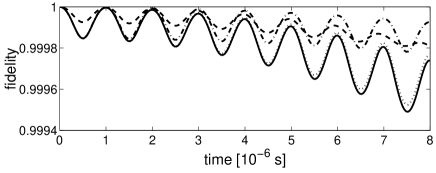
Figure 2: Fidelity between the actually generated state $|\psi(t)\rangle$ and the ideally truncated state $|\psi_{\rm cut}(t)\rangle$ if the coupling strengths are (a) $\epsilon=\alpha$ and (b) $\epsilon=\alpha/10$ for the system pumped in one mode with $\beta=0$ (dashed curves), and that pumped in two modes with: $\beta=\alpha$ (solid), $\beta=-\alpha$ (dotted), $\beta=i\alpha$ (dot-dashed curves). In figures 2–7, we assume that the nonlinearity coefficients are $\chi_{a}=\chi_{b}=10^{8}$ rad/sec, $\alpha=\chi_{a}/200$, and the coupler is initially in two-mode vacuum state $|00\rangle$.

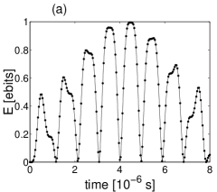
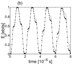
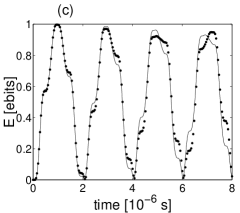
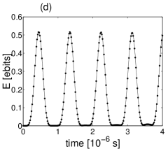
Figure 3: Evolution of the entropy of entanglement $E$ of the generated states $|\psi(t)\rangle$ (dots) and the desired truncated states $|\psi_{\rm cut}(t)\rangle$ (solid curves) by the coupler pumped in a single mode with (a) $\beta=0$ and in two modes with: (b) $\beta=\alpha$, (c) $\beta=-\alpha$, (d) $\beta=i\alpha$, where $\alpha=\epsilon$.

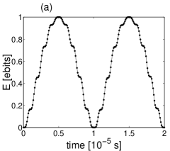
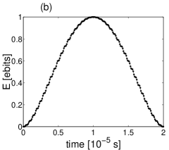
Figure 4: Evolution of the entropy of entanglement $E$ for the coupler pumped in (a) single mode ($\beta=0$) and (b) two modes ($\beta=\alpha$) using line styles and parameters same as in figure 3 except $\epsilon=\alpha/10$. On this figure scale, evolutions of $E$ for $\beta=-\alpha$ can be described by the same curve as in figure (b), while the entropy of entanglement for $\beta=i\alpha$ is negligible as less than $5\times 10^{-4}$.

$$F(\hat{\rho},\hat{\rho}_{\rm cut}) = \left\{{\rm Tr}[(\sqrt{\hat{\rho}_{\rm cut}}\hat{\rho}\sqrt{\hat{\rho}_{\rm cut}})^{1/2}]\right\}^{2}.$$ (15)

By assuming that one of the states is pure (say $|\psi\rangle_{\rm cut}$), then (15) simplifies to $F=\,_{\rm cut}\langle\psi|\hat{\rho}|\psi\rangle_{\rm cut}$. Instead fidelity, the Bures distance $D_{B}(\hat{\rho}||\hat{\rho}_{\rm cut})=2-2\sqrt{F(\hat{\rho},\hat{\rho}_{\rm cut})}$ is often applied as a measure of discrepancy between the states. Note that the Bures distance satisfies the usual metric properties including symmetry $D_{B}(\hat{\rho}||\hat{\rho}_{\rm cut})=D_{B}(\hat{\rho}_{\rm cut}||\hat{\rho})$, contrary to the quantum Kullback-Leibler ‘distance’ (quantum relative entropy) often used in quantum-information context Ved02 . General expression (15) will be applied in our description of the effect of damping on the optical-state truncation in section 4. In this section, we are focused on pure-state truncation, for which equation (15) simplifies to the familiar expression $F=||\langle\psi(t)|\psi(t)\rangle_{\rm cut}||^{2}$, where the ideally truncated state $|\psi(t)\rangle_{\rm cut}$ is given by (10) and the actually generated state $|\psi(t)\rangle$ is calculated numerically from (14). The fidelity for perfect truncation is equal to one. Figure 2 clearly indicates that the fidelity of truncation using the pumped coupler is close to one for short times and the coupling strengths much smaller than the nonlinearity parameters ($|\alpha|,|\epsilon|\ll\chi_{a,b}$). The numerical results shown in figure 2 confirm the validity of our analytical approach at least for short evolution times. Thus, we can refer to the system as a kind of nonlinear (as operating by means of Kerr nonlinearity) quantum scissors device.

Solutions for probability amplitudes of the truncated states enable a simple calculation of quantum entanglement, which is one of the most fundamental resources of quantum information theory Nie00 . It is well known that the entanglement of a bipartite pure state, described by a density matrix $\hat{\rho}=|\psi\rangle\langle\psi|$, can be described by the von Neumann entropy of either the reduced density matrix $\hat{\rho}_{a}={\rm Tr}_{b}\hat{\rho}$ or $\hat{\rho}_{b}={\rm Tr}_{a}\hat{\rho}$ or, equivalently, by the Shannon entropy of the squared Schmidt coefficients $p_{i}$ Ved02 :

$$E(\hat{\rho}) = -{\rm Tr}(\rho_{a}\log_{2}\rho_{a})=-{\rm Tr}(\rho_{b}\log_{2}\rho_{b})$$ (16)

$$= -\sum_{i=1}^{N}p_{i}\log_{2}p_{i}\equiv h(p_{1},...,p_{N-1}).$$

For bipartite pure states this measure is often referred to as the entropy of entanglement. In a special case of two qubits in a pure state, the entropy of entanglement $E$ ranges from zero for a separable state to 1 ebit for a maximally entangled state, and it is simply given in terms of the binary entropy $h(p)=-p\log_{2}p-(1-p)\log_{2}(1-p)$. In fact, for a general two-qubit pure state, given by (10) with arbitrary amplitudes $c_{mn}$ ($m,n=0,1$), the entropy of entanglement given by (16) can simply be calculated as

$$E(t)\equiv E(|\psi(t)\rangle_{\rm cut})={\cal E}\left(2|c_{00}(t)c_{11}(t)-c_{01}(t)c_{10}(t)|\right),$$ (17)

where

$${\cal E}(x)\equiv h\left(\frac{1}{2}(1+\sqrt{1-x^{2}})\right)$$ (18)

and $h$ is the binary entropy. If the probability amplitudes $c_{mn}(t)$ evolve according to (12) then the evolution of the entropy of entanglement is given by

$$E(t)={\cal E}\Big{(}\sum_{j=1,2}\frac{\Omega_{j}}{\gamma^{2}}\big{\{}\epsilon\cos({\textstyle{\frac{1}{2}}}\Omega_{3-j}t)-[\epsilon+(-1)^{j}\gamma]$$

$$\times\cos({\textstyle{\frac{1}{2}}}\Omega_{j}t)\big{\}}\sin({\textstyle{\frac{1}{2}}}\Omega_{3-j}t)\Big{)}.$$ (19)

Solution (19) is further simplified by assuming real $\alpha=\epsilon$ then the amplitudes $c_{mn}$ are given by (13). Thus, we obtain

$$E(t)={\cal E}\Big{(}\frac{1}{5}\{[4+\cos(\sqrt{5}\alpha t)]\sin(\alpha t)$$

$$-\sqrt{5}\cos(\alpha t)\sin(\sqrt{5}\alpha t)\}\Big{)}.$$ (20)

Figures 3(a) and 4(a) show the plots of the entropy of entanglement for the case discussed here, i.e., for the single-mode pumped coupler with the coupling parameters $|\alpha|$ and $|\epsilon|$ much smaller than the nonlinearities $\chi_{a}=\chi_{b}$. We see in figure 3(a) that the rapid oscillations in time (with a period $T_{1}=\pi/|\alpha|$) are modulated by oscillations of low frequency (with period $T_{2}=8\pi/|\alpha|$). As a consequence, their maxima are of various values but some of them approach 1 ebit corresponding to the formation of Bell states. To show this explicitly, we represent the generated state in the basis $|\psi\rangle=\sum_{j=1}^{4}b_{j}|B_{j}\rangle$ spanned by the Bell-like states:

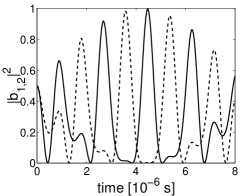
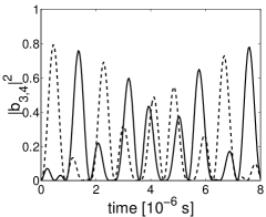
Figure 5: Probabilities $|b_{i}|^{2}$ for finding the coupler pumped in a single mode with $\epsilon=\alpha$ in the Bell states: $|B_{1}\rangle$ and $|B_{3}\rangle$ (solid curves) as well as $|B_{2}\rangle$ and $|B_{4}\rangle$ (dashed curves).

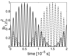
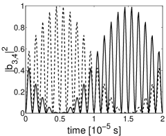
Figure 6: Probabilities for finding the single-mode pumped coupler with $\epsilon=\alpha/10$ in the Bell states. Same symbols as in figure 5.

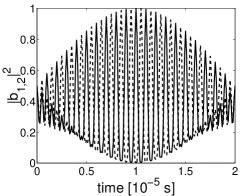
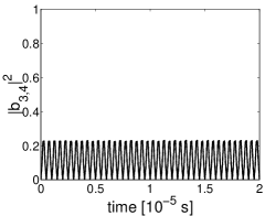
Figure 7: Probabilities for finding the coupler pumped in two modes with $\alpha=\beta$ and $\epsilon=\alpha/10$ in the Bell states. Same symbols as in figure 5.

$$|B_{1}\rangle = \frac{|11\rangle+i|00\rangle}{\sqrt{2}},\quad|B_{2}\rangle\,=\,\frac{|00\rangle+i|11\rangle}{\sqrt{2}},$$

$$|B_{3}\rangle = \frac{|01\rangle-i|10\rangle}{\sqrt{2}},\quad|B_{4}\rangle\,=\,\frac{|10\rangle-i|01\rangle}{\sqrt{2}},$$ (21)

which differ from the standard Bell states only by the phase factor $i$. Clearly, $\sum_{j}|B_{j}\rangle\langle B_{j}|=1$ and $E(|B_{j}\rangle)=1$ for $i=1,...,4$, so states (21) will shortly be referred to as the Bell states. Figures 5 and 6 show the probabilities for the generation of the Bell states as a function of time for the single-mode driven couplers, when the initial state is the two-mode vacuum state. It is seen that states $|B_{1}\rangle$ and $|B_{2}\rangle$, being superpositions of $|00\rangle$ and $|11\rangle$, are generated with a high accuracy. In detail, the maxima of (20) occur approximately at times $t(m,n)=\frac{1}{2}[(2m-1)T_{1}+(2n-1)T_{2}]$ if $\alpha=\epsilon$. Since the frequencies of oscillations in (20) are incommensurate, by waiting long enough (assuming no dissipation), we can achieve 1 ebit with high precision. For example, in the first four periods of $T_{2}$, one could observe generation of entangled states approaching Bell state $|B_{1}\rangle$ with $E[t(1,1)]=0.994$ and $E[t(1,2)]=0.997$ ebits, and approaching $|B_{2}\rangle$ with $E[t(2,3)]=0.992$ and $E[t(2,4)]=0.998$. Note that only the first period is shown in figures 3(a) and 5(a), for which the highest entanglement of 0.994 ebits occurs approximately at the time $t(1,1)=4.5\times 10^{-6}$. Thus, we can effectively treat our system as a source of maximally entangled states. On the other hand, the Bell states $|B_{3}\rangle$ and $|B_{4}\rangle$, being superpositions of $|10\rangle$ and $|01\rangle$, are not generated if the initial state is vacuum and $\epsilon=\alpha$. This conclusion can be drawn by observing that the probabilities for $|B_{3}\rangle$ and $|B_{4}\rangle$ can reach only $0.8$ in figure 5(b). However, by relaxing the condition of equal couplings $\epsilon$ and $\alpha$, as shown in figure 6(b), Bell states $|B_{3}\rangle$ and $|B_{4}\rangle$ can be generated from vacuum with high precision in the dissipation-free system.

Hitherto, we have assumed that both cavity modes were initially in vacuum states. Now, we analyze a more general evolution when the cavity modes are initially not only in vacuum but also in single-photon Fock states, i.e., $|\psi(0)\rangle\equiv|\psi^{(kl)}(0)\rangle=|kl\rangle$, where $k,l=0,1$. Thus, by assuming as usual that $|\alpha|=|\epsilon|\ll\chi_{a},\chi_{b}$, the evolutions of the initial states are found to be

$$|\psi^{(01)}(\tau)\rangle_{\rm cut} = c_{01}|00\rangle+\widetilde{c}_{00}|01\rangle+\widetilde{c}_{11}|10\rangle+c_{10}|11\rangle,$$

$$|\psi^{(10)}(\tau)\rangle_{\rm cut} = c_{10}|00\rangle+\widetilde{c}_{11}|01\rangle+\widetilde{c}_{00}|10\rangle+c_{01}|11\rangle,$$

$$|\psi^{(11)}(\tau)\rangle_{\rm cut} = c_{11}|00\rangle+c_{10}|01\rangle+c_{01}|10\rangle+c_{00}|11\rangle$$

in terms of the time-dependent amplitudes $c_{mn}(\tau)$ given by (13) and

$$\widetilde{c}_{00}(\tau)= \cos(\sqrt{5}\tau)\cos(\tau)-\frac{1}{\sqrt{5}}\sin(\sqrt{5}\tau)\sin(\tau),$$

$$\widetilde{c}_{11}(\tau)= -i\cos(\sqrt{5}\tau)\sin(\tau)-\frac{i}{\sqrt{5}}\sin(\sqrt{5}\tau)\cos(\tau),$$ (23)

where, as usual, $\tau=\alpha t/2$. Please note that $\widetilde{c}_{jj}(\tau)$ and $c_{jj}(\tau)$ differ in sign. We find that the generalized expression for the entropies of entanglement for the initial states $|kl\rangle$ with $k,l=0,1$ reads as

$$E^{(kl)}(t)={\cal E}\Big{(}\frac{1}{5}[4+\cos(\sqrt{5}\alpha t)]\sin(\alpha t)\hskip 42.67912pt$$

$$-(-1)^{k-l}\sqrt{5}\cos(\alpha t)\sin(\sqrt{5}\alpha t)\Big{)},$$ (24)

which implies that

$$E^{(00)}(t) = E^{(11)}(t),$$

$$E^{(01)}(t) = E^{(10)}(t).$$ (25)

It is worth noting that our system for the initial states $|01\rangle$ or $|10\rangle$ quasi-periodically evolves into the Bell states $|B_{3}\rangle$ and $|B_{4}\rangle$ with high precision but does not evolve into $|B_{1}\rangle$ or $|B_{2}\rangle$ assuming $\alpha=\epsilon$. This is by contrast to the evolutions of the initial states $|00\rangle$ (see figure 5) or $|11\rangle$ also for $\epsilon=\alpha$. For brevity, we will not present any graphs of the evolutions of the initial states $|01\rangle$, $|10\rangle$, and $|11\rangle$, which would correspond to figures 2–5 plotted for the initial vacua.

The above solutions for the initial single-photon states are included for completeness of our mathematical approach to show that, in principle, all Bell states can be generated in our system even for $\epsilon=\alpha$. But it should be stressed that the system with the initial Fock states is much more experimentally challenging than that assuming initially the vacuum states only. Despite of experimental difficulty, our system enables generation of the one-photon Fock states from vacuum assuming no coupling $\epsilon$ between the modes, which corresponds to having two independent pumped cavities with nonlinear Kerr media. A possibility of producing single-photon states in such systems was demonstrated in Leo97 (for a review see LM01 and references therein).

3 Coupler pumped in two modes

This section is devoted to the most general scheme presented in figure 1, namely that involving two external excitations. We assume here that both modes of the coupler are excited by external fields, whereas for the case discussed previously we assumed that only one of the modes was coupled to the external field. The Hamiltonian describing such a system is of the form

$$\hat{H}_{1}=\hat{H}^{(a)}_{\rm nonl}+\hat{H}^{(b)}_{\rm nonl}+\hat{H}_{\rm int}+\hat{H}^{(a)}_{\rm ext}+\hat{H}^{(b)}_{\rm ext},$$ (26)

which is the same as that defined by (1)–(4), except for the extra term given by

$$\hat{H}^{(b)}_{\rm ext} = \beta\hat{b}^{\dagger}+\beta^{*}\hat{b}$$ (27)

corresponding to the coupling of the cavity mode $b$ with an external driving single-mode classical field (say, with frequency $\omega_{\rm ext}^{(b)}$), where the parameter $\beta$ describes the strength of this interaction being proportional to the classical field amplitude. The evolution of our system, described by Hamiltonian (26), can be given by the Schrödinger equation from which we find the following set of equations for the amplitudes $c_{mn}(t)$ of the wavefunction (6) in the interaction picture:

$$i\frac{d}{dt}c_{mn}=\left[\chi_{a}m(m-1)+\chi_{b}n(n-1)\right]c_{mn}$$

$$+\epsilon c_{m-1,n+1}\sqrt{m(n+1)}+\epsilon^{\ast}c_{m+1,n-1}\sqrt{(m+1)n}$$

$$+\alpha c_{m-1,n}\sqrt{m}+\alpha^{\ast}c_{m+1,n}\sqrt{m+1}$$

$$+\beta c_{m,n-1}\sqrt{n}+\beta^{\ast}c_{m,n+1}\sqrt{n+1}.$$ (28)

Analogously to the analysis in the former section, we assume short evolution times as well as the couplings $|\alpha|$, $|\beta|$, and $|\epsilon|$ to be much smaller than the Kerr nonlinearities $\chi_{a}$ and $\chi_{b}$. Then, equation (28) for $m,n\neq 0,1$ can be approximated by (8) with the solution (9), which vanishes for the initial condition $c_{mn}(0)=0$. Thus, under the above assumptions, the infinite set of equations (28) reduces to the following four equations:

$$i\frac{dc_{00}}{dt} = \alpha^{*}c_{10}+\beta^{*}c_{01},$$

$$i\frac{dc_{01}}{dt} = \epsilon^{*}c_{10}+\alpha^{*}c_{11}+\beta c_{00},$$

$$i\frac{dc_{10}}{dt} = \epsilon c_{01}+\alpha c_{00}+\beta^{*}c_{11},$$

$$i\frac{dc_{11}}{dt} = \alpha c_{01}+\beta c_{10}.$$ (29)

Assuming that at the time $t=0$, both oscillator modes are in the vacuum states, i.e., $c_{00}=1$ and $c_{01}=c_{10}=c_{11}=0$, we can obtain analytical solutions of (29). To solve (29) we need to find zeros of a fourth-order polynomial and, hence, the solutions in their general form are rather complicated and unreadable. However, if we assume that all coupling constants are real and the couplings with two external fields are of the same strength ($\alpha=\beta$) then the solutions become much simpler and easier to interpret. Thus, under these assumptions, the solutions are found to be:

$$c_{00} = \frac{1}{2}\left\{1+\left[\cos(\frac{\lambda t}{2})+i\frac{\epsilon}{\lambda}\sin(\frac{\lambda t}{2})\right]e^{-i\epsilon t/2}\right\},$$

$$c_{01} = c_{10}=-i2\frac{\alpha}{\lambda}\sin(\frac{\lambda t}{2})\,e^{-i\epsilon t/2},$$

$$c_{11} = c_{00}-1,$$ (30)

where we have introduced the effective coupling constant $\lambda=\sqrt{16\alpha^{2}+\epsilon^{2}}$. As in the case discussed in the previous section, the system’s dynamics is closed within the finite set of $n$-photon states. Figure 2 shows that for the assumed parameters and evolution times shorter than $5\times 10^{-6}$s, the fidelity between the ideally truncated states and the actually generated states by means of the coupler pumped in two modes deviates from 1 by the values less than $0.03$ in figure 2(a) or even $<6\times 10^{-4}$ in figure 2(b). This again confirms the validity of our analysis and justifies referring to this system as a kind of the quantum scissors device. For the parameters assumed in figure 2, truncation with higher fidelity is usually observed for the coupler pumped in a single mode rather than in two modes. In the latter case, the truncation fidelity depends on the relative phase between the pumping-field couplings $\alpha$ and $\beta$. Note that state $|\psi_{\rm cut}\rangle$ for $\beta=\pm\alpha$, contrary to $\beta=i\alpha$, can be directly calculated from solution (12). For brevity, we have not presented here an analogous solution for $\beta=i\alpha$, but we have used it for plotting the corresponding curves in figures 2 and 3(d). It is seen, by comparing figures 2(a) and 2(b), that by decreasing $\epsilon$ in comparison to $\alpha$, the fidelity of truncation can be improved for $\beta\neq 0$. Thus, pumping the coupler in two modes can lead sometimes to truncation better than that for the system driven in single mode as presented in figure 2(b) by dot-dashed curve corresponding to $\beta=i\alpha$ and $\epsilon=\alpha/10$.

The evolution of the pure-state entanglement, given by (16), generated in the coupler pumped in two modes can be calculated from (17) with the probability amplitudes given by (30). Thus, we obtain

$$E(t)={\cal E}\Big{(}\frac{1}{2}\big{|}1-\frac{e^{-i\epsilon t}}{\lambda^{2}}\big{[}16\alpha^{2}+\epsilon^{2}\cos(\lambda t)+i\epsilon\lambda\sin(\lambda t)\big{]}\big{|}\Big{)}.$$ (31)

Figures 3(b-d) and 4(b) show the evolution of the entropy of entanglement measured in ebits as a function of time for the system pumped in two modes in comparison to the results for the single-mode driven coupler shown in figures 3(a) and 4(a). It is seen that the first maximum in figures 3(b-d) is the highest, contrary to the case shown in figures 3(a) for the single-mode pumping. Nevertheless, the most important fact is that the value of the entropy of entanglement $E$ can approach unity to a high precision. So, as in the case of the single-mode pumping, the two-mode driven system effectively generates Bell states. To find which Bell states are generated, we can also transform the resulting wavefunction into the Bell basis. Thus, figure 7 depicts probabilities for the four Bell states. As expected from the form of our analytical solutions for $c_{mn}$ ($m,n=0,1$), the entanglement occurs for the states $|00\rangle$ and $|11\rangle$, and leads to the generation of the states $|B_{1}\rangle$ and $|B_{2}\rangle$ (with some unimportant global phase factor). Clearly, the highest peaks of the entropy $E(t)$ and those of the probabilities $|b_{1,2}(t)|^{2}$ of the Bell state generation occur at the same evolution times, as seen by comparing figures: 3(a) with 5(a), 4(a) with 6(a), and 4(b) with 7. Analysis of the evolutions of the probabilities $|b_{1,2}(t)|^{2}$ and the entropy of entanglement $E(t)$ for relatively longer times reveals that the oscillations are modulated and some long-time oscillations occur in the system, which can be interpreted as a result of quantum beats. It is seen from (31) that two various frequencies appear in our solution and one of them is considerably greater than the other, e.g., the effective coupling constant $\lambda$ is $\sqrt{17}$ times greater than the internal coupling constant of the coupler $\epsilon=\alpha$. We are not presenting here dissipation-free evolutions exhibiting modulated oscillations at times longer than those in figure 4. It would be meaningless since the entanglement is lost at such evolution times due to dissipation, which inevitably occurs in real physical implementations of the coupler as will be discussed in the next section.

Although our analysis, including all figures, is focused on evolution of the initial vacuum states, we present shortly some results for other states too. We find that the evolution of the initial Fock state $|\psi^{(kl)}(0)\rangle=|kl\rangle$ with $k,l=0,1$ is of the form (LABEL:N22) but with the probability amplitudes $c_{mn}(\tau)$ given by (30) and $\widetilde{c}_{mn}(\tau)$ equal to

$$\widetilde{c}_{00}(\tau) = \frac{1}{2}\Big{\{}e^{i\epsilon t}+e^{-i\epsilon t/2}\Big{[}\cos(\frac{\lambda t}{2})-i\frac{\epsilon}{\lambda}\sin(\frac{\lambda t}{2})\Big{]}\Big{\}},$$

$$\widetilde{c}_{11}(\tau) = \widetilde{c}_{00}(\tau)-e^{i\epsilon t}.$$ (32)

With the help of these formulae, we can calculate the entropies of entanglement explicitly as

$$E^{(kl)}(t)={\cal E}\Big{(}\frac{1}{2}\Big{|}1-\lambda^{-2}\exp[-i(2|k-l|+1)\epsilon t]\hskip 14.22636pt$$

$$+\big{[}16\alpha^{2}+\epsilon^{2}\cos(\lambda t)(-1)^{k-l}i\epsilon\lambda\sin(\lambda t)\big{]}\Big{|}\Big{)}$$ (33)

implying the same properties as those given by (25) for the single-mode excited system. We point out that both single- and two-mode pumped couplers for $\alpha=\epsilon$ and the initial states $|01\rangle$ or $|10\rangle$ evolve into the Bell states $|B_{3}\rangle$ and $|B_{4}\rangle$ but do not evolve into $|B_{1}\rangle$ or $|B_{2}\rangle$. This is contrary to the evolutions of the initial vacuum states (or $|11\rangle$) as, for example, presented in figures 5 and 7.

4 Dissipation

In a more realistic description both fields $a$ and $b$ lose their photons from the cavities. According to the standard techniques in theoretical quantum optics, dissipation of our system can be modelled by its coupling to reservoirs (heat baths) as described by the interaction Hamiltonian

$$\hat{H} = \hat{H}_{1}+\hat{H}_{\rm loss},$$ (34)

$$\hat{H}_{\rm loss} = \hat{\Gamma}_{a}\hat{f}(\hat{a},\hat{a}^{{\dagger}})+\hat{\Gamma}_{b}\hat{f}(\hat{b},\hat{b}^{{\dagger}})+{\rm h.c.},$$ (35)

where

$$\hat{\Gamma}_{a}=\sum_{j=0}^{\infty}g_{j}^{(a)}\hat{c}_{j}^{(a)},\quad\hat{\Gamma}_{b}=\sum_{j=0}^{\infty}g_{j}^{(b)}\hat{c}_{j}^{(b)}$$ (36)

are the reservoir operators; $\hat{c}_{j}^{(a,b)}$ are the boson annihilation operators of the reservoir oscillators coupled with mode $a$ or $b$, respectively; $g_{j}^{(a,b)}$ are the coupling constants of the interaction with the reservoirs; $\hat{H}_{1}$ is given either by (1) or (26) dependent on the system analyzed. We assume two kinds of functions $\hat{f}(\hat{a},\hat{a}^{{\dagger}})$ and $\hat{f}(\hat{b},\hat{b}^{{\dagger}})$ to describe standard damping and dephasing.

The standard description of a damped system is obtained for (35) with $\hat{f}(\hat{a},\hat{a}^{{\dagger}})=\hat{a}^{\dagger}$ and $\hat{f}(\hat{b},\hat{b}^{{\dagger}})=\hat{b}^{\dagger}$, or explicitly

$$\hat{H}_{\rm loss} = \hat{\Gamma}_{a}\hat{a}^{{\dagger}}+\hat{\Gamma}_{a}^{{\dagger}}\hat{a}+\hat{\Gamma}_{b}\hat{b}^{{\dagger}}+\hat{\Gamma}_{b}^{{\dagger}}\hat{b},$$ (37)

corresponding to energy transfer between the system and reservoirs. It should be stressed that the process described by (37) leads to combined effect of amplitude and phase damping. The evolution in the Markov approximation of the reduced density operator $\hat{\rho}$ of the two cavity modes after tracing out over the reservoirs can be described in the interaction picture by the following master equation (see, e.g., Gardiner )

$$\frac{d\hat{\rho}}{dt} = -i[\hat{H}_{1},\hat{\rho}]+\hat{\cal L}_{\rm loss}\hat{\rho},$$ (38)

where the Liouvillian

$$\hat{\cal L}_{\rm loss}\hat{\rho}=\frac{\gamma_{a}}{2}([\hat{a}\hat{\rho},\hat{a}^{\dagger}]+[\hat{a},\hat{\rho}\hat{a}^{\dagger}])+\frac{\gamma_{b}}{2}([\hat{b}\hat{\rho},\hat{b}^{\dagger}]$$

$$\quad+[\hat{b},\hat{\rho}\hat{b}^{\dagger}])+\gamma_{a}\bar{n}_{a}[[\hat{a},\hat{\rho}],\hat{a}^{\dagger}]+\gamma_{b}\bar{n}_{b}[[\hat{b},\hat{\rho}],\hat{b}^{\dagger}]$$ (39)

is the usual loss term corresponding to $\hat{H}_{\rm loss}$, given by (37); $\gamma_{k}$ is the damping rate of the $k$th ($k=a,b$) (ring) cavity, and $\bar{n}_{k}=[\exp(\hbar\omega_{k}/k_{B}T)-1]^{-1}$ is the mean number of thermal photons at the reservoir temperature $T$. We will analyze both ‘noisy’reservoirs (at $T>0$ implying $\bar{n}_{a},\bar{n}_{b}>0$) and ‘quiet’ reservoirs (at $T\approx 0$, so $\bar{n}_{a}=\bar{n}_{b}\approx 0$). The latter assumption implies that diffusion of fluctuations from the reservoirs into the system modes is negligible. But still this simplified master equation describes the loss of photons from the system modes to the reservoirs.

One can raise some doubts Alicki against using Liouvillian (39) in a description of lossy anharmonic oscillator models given by (2). Also the approximation of $T=0$ in (39) is problematic. Nevertheless, master equation (38) with Liouvillian (39) and Hamiltonian $\hat{H}_{1}$ set to $\hat{H}^{(a)}_{\rm nonl}$ was used in a number of works both for $T>0$ (see, e.g., Dan89 ; Per90 ; Chat91 ; Tanas ) but also for $T=0$ (see, e.g., Mil86 ; Per88 ; Mil89 ; Dan89 ; Gardiner ; Tanas ). Moreover, the same master equation, given by (38) for $\hat{H}_{1}$ set to (2), for coupled anharmonic oscillators was applied in, e.g., Chat91 ; Per94 . Liouvillian (39) for $T=0$ was also used in (Gardiner p. 210) to describe a model essentially similar to ours comprising a nonlinear system, in which two quantized field modes in a cavity interact with a classical pump field. The standard Liouvillian for $T=0$ was also used in Mil91 to describe a system of Kerr nonlinearity, given by $\hat{H}^{(a)}_{\rm nonl}$, and a parametric amplifier driven by a pulsed classical field. Nevertheless, it should be noted that a realistic master equation for Kerr medium Dun99 ; Haus93 is more complicated.

Phase damping (also referred to as dephasing) can be described by (35) assuming $\hat{f}(\hat{a},\hat{a}^{{\dagger}})=\hat{a}^{{\dagger}}\hat{a}$ and $\hat{f}(\hat{b},\hat{b}^{{\dagger}})=\hat{b}^{{\dagger}}\hat{b}$, which gives the following loss Hamiltonian Gardiner :

$$\hat{H}_{\rm loss} = (\hat{\Gamma}_{a}+\hat{\Gamma}_{a}^{\dagger})\hat{a}^{{\dagger}}\hat{a}+(\hat{\Gamma}_{b}+\hat{\Gamma}_{b}^{\dagger})\hat{b}^{{\dagger}}\hat{b}.$$ (40)

This interaction can be interpreted as a scattering process, where the number of photons remains unchanged contrary to the interaction described by (37). Phase damping is essential in a fully quantum picture of dissipation of our system. As a simple generalization of the Gardiner-Zoller master equation for a single harmonic oscillator (Gardiner , equation (6.1.15)), we describe phase damping of our two-mode nonlinear system by master equation (38) for the Liouvillian

$$\hat{\cal L}_{\rm loss}\hat{\rho}=\frac{\gamma_{a}}{2}(2\bar{n}_{a}+1)[2\hat{a}^{\dagger}\hat{a}\hat{\rho}\hat{a}^{\dagger}\hat{a}-(\hat{a}^{\dagger}\hat{a})^{2}\hat{\rho}-\hat{\rho}(\hat{a}^{\dagger}\hat{a})^{2}]$$

$$\quad+\frac{\gamma_{b}}{2}(2\bar{n}_{b}+1)[2\hat{b}^{\dagger}\hat{b}\hat{\rho}\hat{b}^{\dagger}\hat{b}-(\hat{b}^{\dagger}\hat{b})^{2}\hat{\rho}-\hat{\rho}(\hat{b}^{\dagger}\hat{b})^{2}],$$ (41)

which is significantly different from (39).

To analyze dissipative evolution, governed by master equations (38) for Liouvillians (39) and (41), we apply standard numerical procedures for solving ordinary differential equations with constant coefficients as an exponential series.

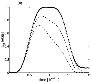
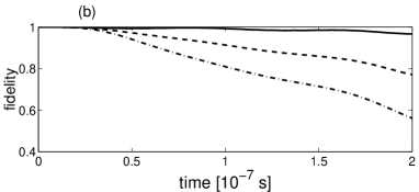
Figure 8: Effect of the standard damping, described by (38) and (39) for quiet reservoirs, on (a) the entanglement of formation and (b) fidelity $F(\hat{\rho},\hat{\rho}_{\rm cut})$, of the states generated in the single-mode pumped coupler from the truncated two-qubit mixed states for $\chi_{a}=\chi_{b}=10^{8}$rad/sec, $\alpha=\chi_{a}/20$, $\epsilon=\alpha/2$, and the damping constants $\gamma_{a}=\gamma_{b}$ equal to 0 (solid), $\chi_{a}/500$ (dashed), and $\chi_{a}/200$ (dot-dashed curves). Large dots in figure (a) correspond to the exact solution.

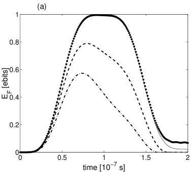
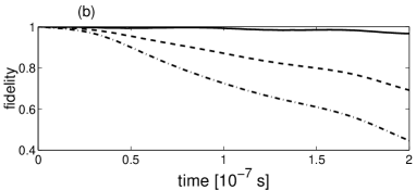
Figure 9: Same as in figure 8 but for noisy reservoirs with mean number $\bar{n}_{a}=\bar{n}_{b}=0.1$ of thermal photons.

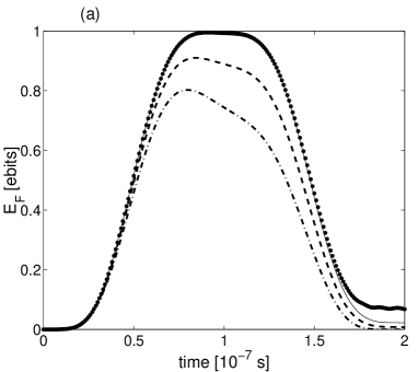
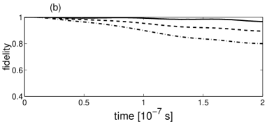
Figure 10: Effect of the phase damping described by (38) and (41) assuming quiet reservoirs for the same parameters as in figure 8.

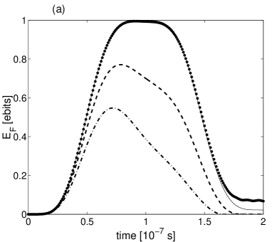
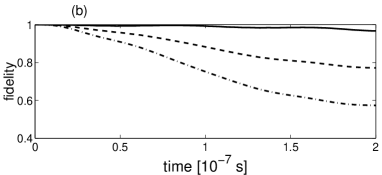
Figure 11: Same as in figure 10 but for noisy reservoirs with $\bar{n}_{a}=\bar{n}_{b}=1$, which is 10 times more than in figure 9.

The entropy of entanglement $E$, given by (16), is valid for qudits of arbitrary dimension in a pure state, but it fails to determine entanglement of a system in a mixed state. Thus, for a two-qubit mixed state $\hat{\rho}$, we have to apply more general measure, e.g., the Wootters measure of entanglement of formation given by Woo98 :

$$E_{F}(\hat{\rho})={\cal E}(C(\hat{\rho})),$$ (42)

where ${\cal E}$ is given by (18) with the argument being the concurrence $C$ defined as

$$C(\hat{\rho})=\max\{2\max_{i}\lambda_{i}-\sum_{i=1}^{4}\lambda_{i},0\},$$ (43)

and $\lambda_{i}$ are the square roots of the eigenvalues of $\hat{\rho}(\hat{\sigma}^{(a)}_{y}\otimes\hat{\sigma}^{(b)}_{y})\hat{\rho}^{\ast}(\hat{\sigma}^{(a)}_{y}\otimes\hat{\sigma}^{(b)}_{y})$, while $\hat{\sigma}^{(k)}_{y}$ is the Pauli spin matrix of the $k$th qubit ($k=a,b$). It is well-known that the entanglement of formation goes into the entropy of entanglement for any two-qubit pure states. Examples of evolution of the entanglement of formation and fidelity for the dissipative systems are shown in figures 8–11 both for quiet and noisy reservoirs. By analyzing the figures, the most important observation is that the generated two-qubit entangled states are very fragile to the leakage of photons from the cavities in the analyzed couplers. Our system is more fragile to losses described by the standard master equation, given by (38) and (39), rather than the losses due to only phase damping as described by the Gardiner-Zoller master equation, given by (38) and (41). Inclusion of reservoir noise, at least for the assumed low mean numbers $\bar{n}\equiv\bar{n}_{a}=\bar{n}_{b}$ of thermal photons, does not cause a dramatic deterioration of fidelity and entanglement in comparison to the losses caused by coupling the system to the zero-temperature reservoirs. Note that we have chosen $\bar{n}=1$ in the dephasing model shown in figure 11 and much smaller value of $\bar{n}$ in the standard dissipation model in figure 9. The reason is that for the latter dissipation model, the number of photons in the system can be increased by absorbing thermal photons from the reservoirs. If this absorption of thermal photons exceeded the loss of the system photons to the reservoirs then the generated fields could not be approximated as two-qubit states and the Wootters function $E_{F}$, given by (42), would fail to be a good entanglement measure. For the parameters chosen in figure 9, the generated states are well approximated by two-qubit density matrices and thus its entanglement of formation is well described by (42). By contrast, the number of system photons is not affected by the reservoirs in the dephasing model; thus (42) can be used for any number $\bar{n}$ of thermal photons.

Finally, it should be noted that fragility of our system to dissipation seems to be a serious drawback from an experimental point of view. Nevertheless, a method which enables a significant improvement of the entanglement robustness of the generated states, has recently been suggested for a similar system Leo05 .

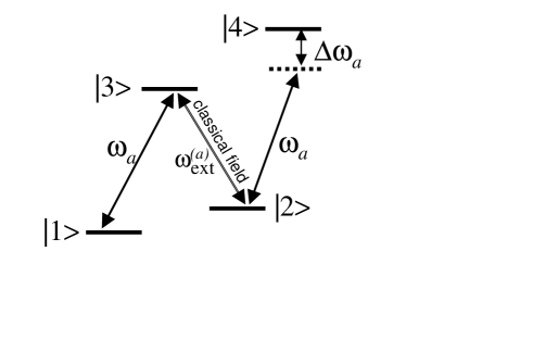
Figure 12: Level structure of atoms in the Schmidt-Imamoǧlu system Sch96 ; Ima97 exhibiting a resonantly enhanced Kerr nonlinearity in mode $a$. An analogous figure can be drawn for mode $b$.

5 Discussion and conclusions

One of the crucial conditions for the successful truncation and generation of the Bell states in our scheme concerns the couplings $|\alpha|$, $|\beta|$ and $|\epsilon|$ to be much smaller than the Kerr nonlinearities $\chi_{a}$ and $\chi_{b}$. This implies that the Kerr interaction should be strong at very low light intensities. Thus, it is desirable to discuss an implementation, in which such stringent conditions can experimentally be satisfied. A possible realization can be based on the effect of the electromagnetically-induced transparency (EIT) or atomic dark resonances as proposed by Schmidt and Imamoǧlu Sch96 ; Ima97 (see also Gra98 ) and observed experimentally Hau99 ; Kan03 . The Schmidt-Imamoǧlu EIT scheme can be realized in a low density system of four-level atoms, which level structure is shown in figure 12, exhibiting giant resonantly-enhanced Kerr nonlinearity at very low intensities. The atoms are placed in cavity $a$ (and analogously in cavity $b$) tuned to frequency $\omega_{a}$ of the mode $a$ resonant with the transition $|1\rangle\leftrightarrow|3\rangle$ and detuned by $\Delta\omega_{a}$ of the transition $|2\rangle\leftrightarrow|4\rangle$. The EIT effect is created by a classical pumping field of frequency $\omega_{\rm ext}^{(a)}$ resonant with the transition $|2\rangle\leftrightarrow|3\rangle$. By assuming $|g_{13}|^{2}n_{\rm atom}/\Omega_{a}^{2}<1$ (see Gra98 ), all the atomic levels can adiabatically be eliminated, which results in the following formula for the Kerr nonlinearity Ima97 :

$$2\chi_{a}\sim\frac{3\hbar\omega_{a}^{2}}{2\epsilon_{0}V_{a}}{\rm Re}(\chi_{a}^{(3)})=\frac{3|g^{(a)}_{13}|^{2}|g^{(a)}_{24}|^{2}}{\Omega^{2}_{a}\Delta\omega_{a}}n_{\rm atom},$$ (44)

where $\chi_{a}^{(3)}$ is third-order nonlinear susceptibility, $g_{ij}=\mu_{ij}\sqrt{\omega_{i}/(2\hbar\epsilon_{0}V_{a})}$ are the coupling coefficients, $\Omega_{a}$ is the Rabi frequency of the classical driving (and coupling) field, $\mu_{ij}$ is the electric dipole matrix element between the states $|i\rangle$ and $|j\rangle$, $n_{\rm atom}$ is the total number of atoms contained in the cavity of volume $V_{a}$, and $\epsilon_{0}$ is the permittivity of free space. By replacing subscript $a$ by $b$ in (44), an analogous expression for $\chi_{b}$ can be obtained. By putting the stringent limit on the required cavity parameters Gra98 , Imamoǧlu et al. estimated $\chi_{a}\sim 10^{8}$ rad/sec Ima97 . Note that some quantum information applications of these giant Kerr nonlinearities have already been studied Dua00 ; Vit00 ; Ott03 ; Baj04 ; Mir04 . More details about application of the Schmidt-Imamoǧlu scheme of resonantly-enhanced Kerr nonlinearity in the analysis of dissipation effects on entanglement generation are given by one of us in Mir04a .

It is worth stressing the differences between the present paper and our former works. (i) In Leo04 ; Leo05 , only the single-mode pumped systems were studied. Here, we analyze also two-mode pumped systems, which is basically a different model. (ii) The model described in Leo05 is crucially different from the one used here as was based on the two-mode nonlinear interaction term $\hat{H}_{\rm int}=\epsilon\hat{a}^{2\dagger}\hat{b}^{2}+{\rm h.c.}$. In the present work, as well as in Leo04 , we apply the two-mode linear interaction Hamiltonian $\hat{H}_{\rm int}=\epsilon\hat{a}^{\dagger}\hat{b}+{\rm h.c.}$, which is the same (by neglecting the pump terms $\hat{H}^{(a)}_{\rm ext}$ and $\hat{H}^{(b)}_{\rm ext}$) as that used in Che96 ; Hor89 ; Kor96 ; Fiu99 ; Ibr00 ; Ari00 ; San03 ; ElOrany05 . The other novelties of the present work in comparison to Leo04 ; Leo05 can be summarized as follows: (1) for single-mode pumped system, we found a new generalized solution (12), which, in a special case of equal couplings $\alpha$ and $\epsilon$, simplifies to our former solution obtained in Leo04 . (2) Analytical approximate solutions were found here for various initial Fock states $|n\rangle$. In Leo04 ; Leo05 , solutions were given for initial vacuum states only. (3) Here, we describe a possible realization of the model based on the effect of the electromagnetically-induced transparency. (4) In present numerical analysis based on the EIT scheme, in comparison to Leo04 ; Leo05 , more realistic parameters were chosen for the coupling constants, Kerr nonlinearities, and damping constants. (5) The deterioration of the fidelity of the generated Bell states due to the standard dissipation and phase damping was analyzed here within two types of master equations both for quiet and noisy reservoirs. By contrast, analysis of losses in Leo04 was limited to the standard master equation and for the quiet reservoir only. No effect of dissipation was studied in Leo05 . (6) In the present manuscript, entanglement of formation was calculated analytically for dissipation-free systems and calculated numerically for dissipative systems. No analytical formulae were given in Leo04 , while the entanglement of formation was not at all studied in Leo05 . (7) The quality of truncation was described here, but it was not studied in Leo04 ; Leo05 . Discrepancy between the really generated states and the exact truncated states was measured here by the fidelity.

In conclusion, we have described a realization of the generalized two-mode optical-state truncation of two coherent modes via a nonlinear process. Our system is a two-mode generalization of the single-mode nonlinear quantum scissors device described in Leo97 . We have described an implementation of the Kerr nonlinear couplers, where resonantly enhanced nonlinearities can be achieved in the Schmidt-Imamoǧlu EIT scheme. We have compared Kerr nonlinear couplers linearly excited in one or two modes by external classical fields. We have shown under assumption of the coupling strengths to be much smaller than the nonlinearity parameters $\chi_{a}$ and $\chi_{b}$ that the optical states generated by the couplers are the two-qubit truncated states spanned by vacuum and single-photon states. Although our approximate solutions of the Schrödinger equation are independent of $\chi$-constants, the Kerr nonlinearity plays a crucial role in the physics as we have derived from the complete $\chi$-dependent Hamiltonian. In fact, the Kerr interaction is the mechanism in our model, which enables truncation of the generated state at some energy level. By contrast, the system without the Kerr nonlinearities and pumped by an external field would gain more and more energy. To confirm our predictions, we have compared ‘exact’ (accurate up to double-precision) direct numerical solutions of the Schrödinger equation and compared with our approximate analytical solutions. The discrepancies between the exact and approximate solutions are relatively small as shown by fidelities in figures 2–4. We have demonstrated that our system initially in vacuum state or single-photon Fock states $|mn\rangle$ ($m,n=0,1$) evolves into Bell states. We have discussed the fragility of the entanglement of formation of the generated states due to the standard dissipation and dephasing in the two distinct master equation approaches.

- (1) Special issue on Quantum State Preparation and Measurement, 1997 J. Mod. Opt. 44 No. 11/12
- (2) Nielsen M A and Chuang I L 2000 Quantum Computation and Quantum Information (Cambridge: University Press)
- (3) Pegg D T, Phillips L S and Barnett S M 1998 Phys. Rev. Lett. 81 1604
- (4) [] Barnett S M and Pegg D T 1999 Phys. Rev. A 60 4965
- (5) Villas-Bôas C J, de Almeida N G, and Moussa M H Y 1999 Phys. Rev. A 60 2759
- (6) Koniorczyk M, Kurucz Z, Gabris A, and Janszky J 2000 Phys. Rev. A 62 013802
- (7) Paris M G A 2000 Phys. Rev. A 62 033813
- (8) Özdemir Ş K, Miranowicz A, Koashi M, and Imoto N 2001 Phys. Rev. A 64 063818
- (9) [] — 2002 Phys Rev A 66 053809
- (10) [] — 2002 J. Mod. Opt. 49 977
- (11) Villas-Bôas C J, Guimarǎes Y, Moussa M H Y, and Baseia B 2001 Phys. Rev. A 63 055801
- (12) Miranowicz A and Leoński W 2004 J. Opt. B: Quantum Semiclass. Opt. 6 S43
- (13) Miranowicz A 2005 J. Opt. B: Quantum Semiclass. Opt. 7 142
- (14) Babichev S A, Ries J, and Lvovsky A I 2003 Europhys. Lett. 64 1
- (15) Resch K J, Lundeen J S, and Steinberg A M 2002 Phys. Rev. Lett. 88 113601
- (16) Leoński W and Tanaś R 1994 Phys. Rev. A 49 R20
- (17) [] Leoński W 1997 Phys. Rev. A 55 3874
- (18) D’Ariano G M, Maccone L, Paris M G A, and Sacchi M F 2000 Phys. Rev. A 61 053817
- (19) Leoński W and Miranowicz A 2004 J. Opt. B: Quantum Semiclass. Opt. 6 S37
- (20) Jensen S M 1982 IEEE J. Quantum Elect. QE-18 1580
- (21) Maier A M 1982 Kvant. Elektron. (Moscow) 9 2996
- (22) Snyder A W, Mitchell D J, Poladian L, Rowland D R, and Chen Y 1991 J. Opt. Soc. Am. B 8 2102
- (23) Grygiel K and Szlachetka P 2001 J. Opt. B: Quant. Semiclass. Opt. 3 104
- (24) Peřina J Jr and Peřina J 2000 Progress in Optics, ed. E Wolf (Amsterdam: Elsevier) 41 361
- (25) Chefles A and Barnett S M 1996 J. Mod. Opt. 43 709
- (26) Horak R, Sibilia C, Bertolotti M, and Peřina J 1989 J. Opt. Soc. B 6 199
- (27) Korolkova N and Peřina J 1997 Opt. Commun. 136 135
- (28) Fiurášek J, Křepelka J, and Peřina J 1999 Opt. Commun. 167 115
- (29) Ibrahim A -B M A, Umarov B A, Wahiddin M R B 2000 Phys. Rev. A 61 043804
- (30) Ariunbold G and Perina J 2000 Opt. Commun. 176 149
- (31) Sanz L, Angelo R M, and Furuya K 2003 J. Phys. A: Math. Gen. 36, 9737
- (32) El-Orany F A A, Sebawe Abdalla M and Peřina J 2005 Eur. Phys. J. D 33 453
- (33) Herec J, Fiurášek J and Mišta L Jr 2003 J. Opt. B: Quant. Semiclass. Opt. 5 419
- (34) Miranowicz A, Leoński W, and Imoto N 2001 Adv. Chem. Phys. (New York: Wiley) 119(I) 155
- (35) Leoński W and Miranowicz A 2001 Adv. Chem. Phys. (New York: Wiley) 119(I) 195
- (36) Vedral V 2002 Rev. Mod. Phys. 74 197
- (37) Gardiner C W and Zoller P 2000 Quantum Noise (Berlin: Springer)
- (38) Alicki R, private communication.
- (39) Daniel D J and Milburn G J 1989 Phys. Rev. A 39 4628
- (40) Peřinová V and Lukš A 1990 Phys. Rev. A 41 414
- (41) Chaturvedi S and Srinivasan V 1991 Phys. Rev. A 43 4054
- (42) Tanaś R 2003 Theory of Non-Classical States of Light, eds V Dodonov and V I Man’ko (London: Taylor & Francis) p 267
- (43) Milburn G J and Holmes C A 1986 Phys. Rev. Lett. 56 2237
- (44) Peřinová V and Lukš A 1988 J. Mod. Opt. 35 1513
- (45) Milburn G J, Mecozzi A, and Tombesi P 1989 J. Mod. Opt. 36 1607
- (46) Peřinová V and Lukš A 1994 Progress in Optics vol 33, ed E Wolf (Amsterdam: North-Holland) p 129
- (47) Milburn G J and Holmes C A 1991 Phys. Rev. A 44 4704
- (48) A. M. Dunlop, W. J. Firth, and E. M. Wright 1999 Optics Express 2 204
- (49) Haus H A, Moores J D, and Nelson L E 1993 Opt. Lett. 18 51
- (50) Wootters W K 1998 Phys. Rev. Lett. 80 2245
- (51) Leoński W and Kowalewska-Kudłaszyk A 2005 Acta Phys. Hung. A 23 55
- (52) Schmidt H and Imamoǧlu A 1996 Opt. Lett. 21 1936
- (53) Imamoǧlu A, Schmidt H, Woods G, and Deutsch M 1997 Phys. Rev. Lett. 79 1467
- (54) [] — 1998 Phys. Rev. Lett. 81 2836
- (55) Grangier P, Walls D F, and Gheri K M 1998 Phys. Rev. Lett. 81 2833
- (56) Hau L V, Harris S E, Dutton Z, and Behroozi C H 1999 Nature (London) 397 594
- (57) Kang H and Zhu Y 2003 Phys. Rev. Lett. 91 093601
- (58) Duan L -M, Giedke G, Cirac J I, and Zoller P 2000 Phys. Rev. Lett. 84 4002
- (59) Vitali D, Fortunato M, and Tombesi P 2000 Phys. Rev. Lett. 85 445
- (60) Ottaviani C, Vitali D, Artoni M, Cataliotti F, and Tombesi P 2003 Phys. Rev. Lett. 90 197902
- (61) Bajer J, Miranowicz A and Andrzejewski M 2004 J. Opt. B: Quantum Semiclass. Opt. 6 387
- (62) Miranowicz A 2004 J. Phys. A: Math. Gen. 37 7909