Quantum algorithms with fixed points:
The case of database search

Abstract

The standard quantum search algorithm lacks a feature, enjoyed by many classical algorithms, of having a fixed-point, i.e. a monotonic convergence towards the solution. Here we present two variations of the quantum search algorithm, which get around this limitation. The first replaces selective inversions in the algorithm by selective phase shifts of $\frac{\pi}{3}$. The second controls the selective inversion operations using two ancilla qubits, and irreversible measurement operations on the ancilla qubits drive the starting state towards the target state. Using $q$ oracle queries, these variations reduce the probability of finding a non-target state from $\epsilon$ to $\epsilon^{2q+1}$, which is asymptotically optimal. Similar ideas can lead to robust quantum algorithms, and provide conceptually new schemes for error correction.

I Introduction

The quantum search algorithm is like baking a souffle …you have to stop at just the right time or else it gets burnt. brass_science

The quantum search algorithm grover96 consists of an iterative sequence of selective inversion and diffusion type operations. Each iteration results in a fixed rotation (which is a function of the initial error probability) of the quantum state in a two-dimensional Hilbert space formed by the source and the target states. The iterative procedure keeps the rotation going forever at a uniform rate. If we choose the right number of iteration steps, we stop very close to the target state, else we keep on going round and round in the two-dimensional Hilbert space. To perform optimally, therefore, we need to know the precise number of iteration steps, which depends upon the initial error probability or equivalently the fraction of target states in the database. When we have this information, the quantum algorithm leads to a square-root speed up over the corresponding classical algorithm for many applications, including unsorted database search. When this information is missing, we can estimate the required number of iteration steps using various “amplitude estimation” algorithms bhmt ; grover98 , but that necessitates an overhead of additional queries. When the total number of queries is large, the additional queries do not cost much, but when the total number of queries is small, the overhead can be unacceptably large.

In this article, we address the problem of finding an optimal quantum search algorithm in situations where, (i) we do not know the initial error probability (perhaps only its distribution or a bound is known), and (ii) the expected number of queries is small (so that every additional query is a substantial overhead). Such situations occur in pattern recognition and image analysis problems (where each query is a significant cost), and in problems of error correction and associative memory recall (where the initial error probability is small but unknown). We look for variations of the quantum search algorithm that ensure amplitude enhancement, and also outperform classical search algorithms.

The strategy is familiar from classical computation, i.e. construct a quantum algorithm that “converges” towards the target state. That is, however, impossible to do by iterating a non-trivial unitary transformation; eigenvalues of unitary transformations are of magnitude 1, so the best that can be achieved by iterating them is a “limit cycle” and not a “fixed point”. As described above, this is indeed what happens in case of the quantum search algorithm. To obtain an algorithm that converges towards a fixed point, some new ingredient is needed, and several possibilities come to mind:
(a) Some property of the current computational state offers an estimate of the distance to the target state. This estimate can be used as a parameter to control the extent of the next iterative transformation, e.g. the Newton-Raphson method to find the zeroes of a function. If such an estimate is not available, we have to look for a different method.
(b) Suitably designed but distinct operations are performed at successive iterations. Such a method can converge towards a fixed point even using unitary transformations. We illustrate this method using the Phase-$\pi/3$ search algorithm pi3 , described in detail in Section II.
(c) Irreversible damping is introduced in the algorithm without explicit use of any property of the target state. With the right type of irreversibility (i.e. when all eigenvalues of the fixed iterative transformation are less than 1 in magnitude), the algorithm converges, e.g. the Gauss-Seidel method for solving a set of linear algebraic equations. Within the framework of quantum computation, such an irreversibility can be introduced by projective measurement operations, and we provide such an algorithm in Section III tath .

In a broader context, fixed point algorithms possess two attractive features by construction, which are not commonplace in generic quantum algorithms:
(1) The initial state is guaranteed to evolve towards the target state, even when the algorithm is not run to its full completion.
(2) Any errors due to imperfect transformations in earlier iterations are wiped out by the subsequent iterations, as long as the state remains in the problem defining space.
These are powerful motivations to explore quantum fixed point algorithms, even if they have other limitations.

Let us consider an unsorted database in which a fraction $f$ of items are marked, but we don’t have precise knowledge of $f$. We run a particular algorithm which has to return a single item from the database. If the returned item is a marked one, the algorithm has succeeded, otherwise it is in error. Without applying any algorithm, if we pick an item at random, then the probability of error is $\epsilon=1-f$. The goal of the algorithm is to minimize the error probability, using the smallest number of oracle queries. If $f$ is sufficiently small, then we can use the optimal quantum search algorithm to obtain a marked item using $O(1/\sqrt{f})$ queries. A few more queries to estimate $f$ or to fine-tune the algorithm is not a problem, because overall we gain a quadratic speed-up compared to the classical case requiring exhaustive search. But when $f$ is large, the number of oracle queries is small, and the quantum search algorithm doesn’t provide much advantage—in particular the rotation can overshoot the target state. In such a situation, a simple classical algorithm (select a random item and use a query to check if it is a marked one) may outperform the quantum search algorithm. The same considerations apply to the more general amplitude amplification algorithms bhmt ; grover98 . There the initial quantum state is a unitary operator $U$ applied to a given source state $|{s}\rangle$, and the probability of getting a target state after measuring this initial state, $|U_{ts}|^{2}$, is analogous to $f$. The probability of error, which has to be minimized using the smallest number of queries, is the probability of getting a non-target state after measurement, $\epsilon=1-|U_{ts}|^{2}$.

In Section II, we show that by replacing the selective phase inversions in quantum search by suitable phase shifts we can get an algorithm that always produces amplitude amplification. As shown in Fig.1, the change in phase shift eliminates overshooting and the state vector always moves closer to the target state. By recursively applying the single iteration derived for any unitary operator $U$, we develop an algorithm with multiple applications of $U$ that converges monotonically to the target state. The optimal value of the phase shift turns out to be $\pi/3$, and we refer to this algorithm as the “Phase-$\pi/3$ search” pi3 . Remarkably, the algorithm converges using reversible unitary transformations and without ever estimating the distance of the current state from the target state. Explicitly, the initial error probability $\epsilon$ changes to $\epsilon^{3}$ in one iteration. Recursive application of the basic iteration $n$ times requires $q_{i}=3q_{i-1}+1$ ($q_{0}=0$) oracle queries at the $i^{\mathrm{th}}$ level, and makes the error probability $\epsilon^{3^{n}}$. Thus $\epsilon=0$ is the fixed point of the algorithm, and the error probability decreases as $\epsilon^{2q+1}$ as a function of the number of queries $q$.

Section III describes a different implementation of the fixed point quantum search, where irreversible measurement operations direct the current state towards the target state tath . In it the inversion and diffusion operations are controlled in a special way by two ancilla qubits and their measurement. The same transformation is repeated at every iteration, but since the transformation is made non-unitary by measurement, the quantum state is able to monotonically converge towards the target state. A major advantage of this implementation is that the $\epsilon^{2q+1}$ convergence is achieved for all positive integer values of $q$, compared to the restricted numbers $q_{n}=(3^{n}-1)/2$ for the Phase-$\pi/3$ search.

Note that the best classical algorithm can only decrease the error probability as $\epsilon^{q+1}$ (not $\epsilon^{q}$, since the last iteration does not need a query). Thus the fixed point quantum search improves the convergence rate by a factor of 2. In Section IV, we illustrate this difference with an explicit example.

Figure 1: In the standard quantum search algorithm (left), the state vector may overshoot the target state. In the algorithm of Section II (right), the state vector always moves towards the target state.

II The Phase-$\pi/3$ Search

Consider applying the transformation

$$O(\theta,\phi)=UR_{s}^{\theta}U^{\dagger}R_{t}^{\phi}U~{},$$ (1)

to the state $|{s}\rangle$, where $R_{s}^{\theta}$ and $R_{t}^{\phi}$ are selective phase shift operators for the source and the target state respectively. Note that if we were to choose the phase shifts as $\theta=\phi=\pi$, we would get one iteration of the amplitude amplification algorithm bhmt ; grover98 .

In the following, we study the particular case $\theta=\phi=\pi/3$. We show that when the $U$ operation drives the state vector from $|s\rangle$ to $|t\rangle$ with a probability $(1-\epsilon)$, i.e. $|U_{ts}|^{2}=(1-\epsilon)$, then $O(\pi/3,\pi/3)$ drives the state vector from the source state to the same target state with a probability of $(1-\epsilon^{3}).$ The deviation from $|t\rangle$ hence falls from $\epsilon$ to $\epsilon^{3}$. The striking aspect of this result is that it holds for any kind of deviation from $|t\rangle$. Unlike the standard quantum search algorithm, which would overshoot the target state when $\epsilon$ is small (Fig.1), the Phase-$\pi/3$ search always moves towards the target state. This property is useful in developing quantum algorithms that are robust to variations in the problem parameters.

Connections to error correction are already evident in the previous paragraph. Let us say that we want to drive a system from $|s\rangle$ to $|t\rangle$ state/subspace, using the transformation $U$, with driving probability $|U_{ts}|^{2}=(1-\epsilon)$. Then the composite transformation $O(\pi/3,\pi/3)$ will reduce the error from $\epsilon$ to $\epsilon^{3}$. This technique is applicable whenever the transformations $U$, $U^{\dagger}$, $R_{s}$ and $R_{t}$ can be implemented. That will be the case when the errors are either systematic or slowly varying, and the transformation $U$ can be inverted with exactly the same error, e.g. when the errors are due to environmental degradation of some component. The technique would not apply to errors that arise as a result of sudden disturbances from the environment. Quantum error correction is carried out at the single qubit level in many implementations, where individual errors are corrected by identifying the corresponding error syndrome. With the machinery of this paper, errors can be corrected without ever needing to identify the error syndrome.

II.1 Analysis

Now let us analyze the effect of the transformation $O(\pi/3,\pi/3)$ when it is applied to the state $|s\rangle$. We want to show that

$$\Big{|}\langle t|UR_{s}^{\pi/3}U^{\dagger}R_{t}^{\pi/3}U|s\rangle\Big{|}^{2}=1-\epsilon^{3}~{}.$$ (2)

Applying the operations, $U$, $R_{s}^{\pi/3}$, $U^{\dagger}$, $R_{t}^{\pi/3}$ and $U$, one by one, to the state $|s\rangle$, we find that

$$O(\pi/3,\pi/3)|s\rangle=U|s\rangle\left(e^{i\pi/3}+|U_{ts}|^{2}\left(e^{i\pi/3}-1\right)^{2}\right)+|t\rangle U_{ts}\left(e^{i\pi/3}-1\right)~{}.$$ (3)

The deviation of this superposition from the target state $|t\rangle$ is given by the absolute square of its overlap with the non-target states. This probability is

$$\Big{|}\langle t_{\perp}|O(\pi/3,\pi/3)|s\rangle\Big{|}^{2} = \langle s|O(\pi/3,\pi/3)^{\dagger}\Big{(}1-|t\rangle\langle t|\Big{)}O(\pi/3,\pi/3)|s\rangle$$ (4)

$$= \left(1-\left|U_{ts}\right|^{2}\right)\left|\left(e^{i\pi/3}+\left|U_{ts}\right|^{2}\left(e^{i\pi/3}-1\right)^{2}\right)\right|^{2}~{}.$$

Substituting $\left|U_{ts}\right|^{2}=(1-\epsilon)$, the above quantity becomes

$$\epsilon\left|\left(e^{i\pi/3}+\left(1-\epsilon\right)\left(e^{i\pi/3}-1\right)^{2}\right)\right|^{2}=\epsilon\left|\left(e^{2i\pi/3}-e^{i\pi/3}+1\right)-\epsilon\left(e^{i\pi/3}-1\right)^{2}\right|^{2}=\epsilon^{3}~{}.$$ (5)

We now use this result recursively to construct the quantum algorithm for searching in presence of uncertainty.

II.2 Recursion

A few years after its invention, the quantum search algorithm grover96 ; sch was generalized to a much larger class of applications known as the amplitude amplification algorithms bhmt ; grover98 . In these algorithms, the amplitude to go from the state $|s\rangle$ to the state $|t\rangle$ by applying a unitary operation $U$, can be amplified by repeating the sequence of operations, $Q=I_{s}U^{{\dagger}}I_{t}U$, where $I_{s}$ and $I_{t}$ denote selective inversions of the $|s\rangle$ and $|t\rangle$ states respectively. Note that the amplitude amplification transformation with four queries is

$$U\left(I_{s}U^{\dagger}I_{t}U\right)\left(I_{s}U^{\dagger}I_{t}U\right)\left(I_{s}U^{\dagger}I_{t}U\right)\left(I_{s}U^{\dagger}I_{t}U\right)~{}.$$ (6)

When the operation sequence $I_{s}U^{{\dagger}}I_{t}U$ is repeated $\eta$ times, the amplitude in the $U^{\dagger}|t\rangle$ state becomes approximately 2$\eta U_{ts}$ provided $\eta U_{ts}\ll 1$. The quantum search algorithm is a particular case of amplitude amplification, with $U$ being the Walsh-Hadamard transformation and $|s\rangle$ being the $|\overline{0}\rangle$ state with all qubits in the $|0\rangle$ state. The selective inversions enable the amplitudes produced by successive iterations to add up in phase. Consequently, the amount of amplification grows linearly with the number of repetitions of $Q$, and the probability of obtaining $|t\rangle$ goes up quadratically.

Just like the amplitude amplification transformation, it is possible to recurse the transformation $UR_{s}U^{\dagger}R_{t}U$ to obtain larger rotations of the state vector in a carefully defined two dimensional Hilbert space. The basic idea is to define transformations $U_{i}$ by the recursion

$$U_{i+1}=U_{i}R_{s}U_{i}^{\dagger}R_{t}U_{i}~{},~{}~{}U_{0}\equiv U~{}.$$ (7)

Unlike amplitude amplification, there is no simple structure in the recursion, and it is not easy to write down the actual operation sequence for $U_{i}$ with large $i$, without working out the full recursion for all integers less than $i$. Let us illustrate this for $U_{2}$:

$$U_{0}=U~{},~{}~{}U_{1}=U_{0}R_{s}U_{0}^{\dagger}R_{t}U_{0}=UR_{s}U^{\dagger}R_{t}U~{},$$ (8)

$$U_{2}=U_{1}R_{s}U_{1}^{\dagger}R_{t}U_{1} = \left(UR_{s}U^{\dagger}R_{t}U\right)R_{s}\left(UR_{s}U^{\dagger}R_{t}U\right)^{\dagger}R_{t}\left(UR_{s}U^{\dagger}R_{t}U\right)$$ (9)

$$= \left(UR_{s}U^{\dagger}R_{t}U\right)R_{s}\left(U^{\dagger}R_{t}^{\dagger}UR_{s}^{\dagger}U^{\dagger}\right)R_{t}\left(UR_{s}U^{\dagger}R_{t}U\right)$$

$$= U\left(R_{s}U^{\dagger}R_{t}U\right)\left(R_{s}U^{\dagger}R_{t}^{\dagger}U\right)\left(R_{s}^{\dagger}U^{\dagger}R_{t}U\right)\left(R_{s}U^{\dagger}R_{t}U\right)~{}.$$

This is not as simple as the corresponding transformation for amplitude amplification, Eq.(6).

Now it is straightforward to show that if $|U_{ts}|^{2}=1-\epsilon$, then $|(U_{i})_{ts}|^{2}=1-\epsilon^{3^{i}}$. The recursion obeyed by the number of queries is, $q_{i+1}=3q_{i}+1$, $q_{0}=0$, with the solution $q_{i}=(3^{i}-1)/2$. As a function of the number of queries, therefore, $|(U_{i})_{ts}|^{2}=1-\epsilon^{2q_{i}+1}$. The error probability thus falls as $\epsilon^{2q+1}$ after $q$ queries, which is an improvement over the classical algorithm where the error probability is $\epsilon^{q+1}$ after $q$ queries (more details in Section IV).

II.3 Fixed Point of the Algorithm

First, note that both the amplitude amplification algorithm, Eq.(6), and the phase shift algorithm, Eq.(9), perform selective operations for the state $|t\rangle$, and so from an information theoretic point of view there is no conflict in having fixed points. However, unitarity would be violated if there was accumulation of the target state due to repetition of a fixed transformation. In the amplitude amplification algorithm, exactly the same transformation is repeated and so unitarity does not permit any fixed point. Although the phase shift algorithm is very similar to the amplitude amplification algorithm, the transformation applied at each step is slightly different from the others, due to the presence of the four operations $R_{s},R_{t},R_{s}^{\dagger},R_{t}^{\dagger}$. It therefore gets around the unitarity condition that prevents the amplitude amplification algorithm from having a fixed point.

The $\epsilon^{2q+1}$ performance of the Phase-$\pi/3$ algorithm has been shown to be asymptotically (i.e. in the limit $\epsilon\rightarrow 0$) optimal jai . It can be shown that application of the general operator $O(\theta,\phi)$ to $|{s}\rangle$ changes its component along $|t_{\perp}\rangle$ by the scale factor $\Big{|}\exp({i\over 2}(\theta-\phi))-4\sin{\theta\over 2}\sin{\phi\over 2}|U_{ts}|^{2}\Big{|}$. In the asymptotic limit, $|U_{ts}|\rightarrow 1$, and the scale factor is minimized by the choice $\theta=\phi={\pi\over 3}$.

III Measurement Based Search Algorithm

To obtain a fixed point quantum search, we have to find an algorithm that successively decreases the probability of finding a non-target state. Let us say that the initial state of a quantum register is $U|{s}\rangle=\sin\alpha|{t}\rangle+\cos\alpha|{t_{\perp}}\rangle$—an unspecified superposition of the target $|t\rangle$ and the non-target $|t_{\perp}\rangle$ states. We can construct a fixed point search algorithm by repetitively measuring the state—whenever the oracle query identifies the measured state as the target state, we stop the algorithm, otherwise we use the diffusion operation to rotate the non-target state towards the target state. To implement this idea, we attach to the quantum register an ancilla bit in the initial state $|{0}\rangle$. The oracle query flips the ancilla when the register is in the target state. Now if we measure the ancilla, outcome $1$ tells us that we are done, and the register will give us the target state. Outcome $0$ tells us that the register is in a superposition $|t_{\perp}\rangle$ of the non-target states, and its probability is the initial error probability $\epsilon=\cos^{2}\alpha$. To decrease this probability, we apply the diffusion operator $UI_{s}U^{\dagger}$ to the register, conditioned on the measurement outcome being $0$. That reflects $|{t_{\perp}}\rangle|{0}\rangle$ about $U|{s}\rangle|{0}\rangle$ to give the state $\sin 2\alpha|{t}\rangle|{0}\rangle+\cos 2\alpha|{t_{\perp}}\rangle|{0}\rangle$. The error probability has thus decreased by the factor $\cos^{2}2\alpha$. Iterating the sequence of oracle query and diffusion operations $n$ times, the error probability is reduced to $\cos^{2}\alpha\cos^{2n}2\alpha=\epsilon(2\epsilon-1)^{2n}$. This convergence is better than the Phase-$\pi/3$ search when $\epsilon>1/3$, but worse when $\epsilon<1/3$.

Our goal is to find an algorithm which gives optimal convergence for all values of $\epsilon$, without knowing any bounds that $\epsilon$ may obey. We know that the rotation provided by a single iteration of the quantum search algorithm overshoots the target state when $\epsilon$ is small. In particular, when $\epsilon$ is less than $1/2$, the overshooting is so large that the new state has a smaller overlap with the target state than the initial state. That gives an inkling for constructing a better directed quantum search—somehow set a lower bound of $1/2$ for $\epsilon$. The natural lower bound for $\epsilon$ is $0$, but we can easily make it $1/2$ by diluting the database with extraneous states. Explicitly, we add to the quantum register a second ancilla in the state $|{+}\rangle\equiv(|{0}\rangle+|{1}\rangle)/\sqrt{2}$, and make the oracle query conditional on this ancilla. This logic produces the following $q$-iteration algorithm:

• Attach two ancilla qubits in the $|0\rangle$ state to the source state $|s\rangle$, i.e. $|s\rangle\rightarrow|0\rangle|s\rangle|0\rangle$. (In what follows, we refer to the former ancilla as ancilla-1 and the latter ancilla as ancilla-2.)

• Apply $H\otimes U\otimes I$ to this extended register to prepare the initial state of the algorithm, $|+\rangle(U|s\rangle)|0\rangle$.

• Iterate the following two steps, $q$ times:
  Step 1: If ancilla-1 is in the state $|1\rangle$, then perform an oracle query that flips ancilla-2 when the register is in target state.
  Step 2: Measure ancilla-2. If the outcome is $1$, the register is certainly in the target state, so exit the iteration loop. If the outcome is $0$, then apply the joint diffusion operator $(H\otimes U)I_{0s}(H\otimes U)^{\dagger}$ to the joint state of ancilla-1 and the register.

• After exiting or completing the iteration loop, stop the algorithm and measure the register.

The quantum circuit for this algorithm is shown in Fig.2.

Figure 2: Quantum circuit for our $q$-iteration algorithm.

III.1 Analysis

Let us analyze the algorithm step by step. The initial state is

$$|{\psi_{i}}\rangle=(H\otimes U\otimes I)|{0}\rangle|{s}\rangle|{0}\rangle=\left(\frac{|{0}\rangle+|{1}\rangle}{\sqrt{2}}\right)\Big{(}\sin\alpha|{t}\rangle+\cos\alpha|{t_{\perp}}\rangle\Big{)}|{0}\rangle~{}.$$ (10)

The initial error probability is $\epsilon=\cos^{2}\alpha$, and the initial success probability is $f=1-\epsilon=\sin^{2}\alpha$. We work in the joint search space of ancilla-1 and the register, denoted by the subscript $j$, where only the state $|{t_{j}}\rangle\equiv|{1}\rangle|{t}\rangle$ acts as the target state and all the states $|{0}\rangle|{t}\rangle,|{0}\rangle|{t_{\perp}}\rangle,|{1}\rangle|{t_{\perp}}\rangle$ act as non-target states. Let $|{t^{\prime}_{j}}\rangle$ denote the superposition of all the non-target states. In the joint search space, the initial state is

$$|{\psi_{i}}\rangle=\left(\frac{\sin\alpha}{\sqrt{2}}\right)|{t_{j}}\rangle|{0}\rangle+\frac{1}{N}|{t^{\prime}_{j}}\rangle|{0}\rangle~{},$$ (11)

where the unit vector $|t^{\prime}_{j}\rangle$ is

$$|{t^{\prime}_{j}}\rangle=N\left(\frac{\sin\alpha}{\sqrt{2}}|{0}\rangle|{t}\rangle+\frac{\cos\alpha}{\sqrt{2}}|{0}\rangle|{t_{\perp}}\rangle+\frac{\cos\alpha}{\sqrt{2}}|{1}\rangle|{t_{\perp}}\rangle\right)~{},$$ (12)

and the normalization constant $N$ is $\left(\cos^{2}\alpha+\frac{1}{2}\sin^{2}\alpha\right)^{-1/2}=\sqrt{2/(1+\epsilon)}$. For later reference, note that the error probability after measuring the joint state $|{t^{\prime}_{j}}\rangle$, i.e. the probability of finding the register in the non-target state $|{t_{\perp}}\rangle$, is

$$|\langle 0|\langle t_{\perp}|t^{\prime}_{j}\rangle|^{2}+|\langle 1|\langle t_{\perp}|t^{\prime}_{j}\rangle|^{2}=N^{2}\cos^{2}\alpha=N^{2}\epsilon~{}.$$ (13)

Step 1 of the algorithm, using an oracle query, flips ancilla-2 when the joint register state is $|{t_{j}}\rangle$. In step 2, we measure ancilla-2. If the outcome is $1$ then we stop the algorithm, because the register is in the target state. The probability of getting $1$ is $\sin^{2}\alpha/2=f/2$; we have effectively put an upper bound of $1/2$ on the success probability using ancilla-1. If the outcome is $0$, which has probability $1/N^{2}$, then the joint state is $|{t^{\prime}_{j}}\rangle$. In this case, we apply the joint diffusion operation using the joint source state $|{s_{j}}\rangle\equiv|{0}\rangle|{s}\rangle$. The joint diffusion operation is a reflection about $(H\otimes U)|0\rangle|s\rangle\equiv U_{j}|s_{j}\rangle$, in the two-dimensional Hilbert space spanned by $|{t_{j}}\rangle$ and $|{t^{\prime}_{j}}\rangle$ as shown in Fig.3. The state $U_{j}|{s_{j}}\rangle$ makes an angle $\alpha_{j}$, defined by $\sin^{2}\alpha_{j}=\sin^{2}\alpha/2$, with the state $|{t^{\prime}_{j}}\rangle$. So reflecting $|{t^{\prime}_{j}}\rangle$ about $U_{j}|{s_{j}}\rangle$ gives us a state that makes an angle $2\alpha_{j}$ with $|{t^{\prime}_{j}}\rangle$. Its component in $|{t^{\prime}_{j}}\rangle$-direction is $\cos 2\alpha_{j}=1-2\sin^{2}\alpha_{j}=1-\sin^{2}\alpha=\epsilon$. Thus the joint diffusion operation produces the final state

$$|{\psi_{f}}\rangle=U_{j}I_{s_{j}}U_{j}^{\dagger}|t^{\prime}_{j}\rangle=\sqrt{1-\epsilon^{2}}|{t_{j}}\rangle+\epsilon|{t^{\prime}_{j}}\rangle~{}.$$ (14)

After measuring $|{\psi_{f}}\rangle$, the probability of getting $|{t^{\prime}_{j}}\rangle$ is $\epsilon^{2}$, so the total probability of getting $|{t^{\prime}_{j}}\rangle$ after one iteration is $N^{-2}\epsilon^{2}$. Iterating the algorithm will keep on decreasing this probability by a factor of $\epsilon^{2}$ at each iteration, and after $q$ iterations it will become $N^{-2}\epsilon^{2q}$. So the net error probability after $q$ iterations is (cf. Eq.(13))

$$\epsilon_{q}=N^{2}\epsilon(N^{-2}\epsilon^{2q})=\epsilon^{2q+1}~{},$$ (15)

which agrees exactly with the corresponding result for the Phase-$\pi/3$ search.

Figure 3: Step-by-step quantum state evolution in our $q$-iteration algorithm. The double arrows relate the equivalent states in the original search space (left) and the joint search space (right).

The above analysis allows us to also deduce the following features:
(1) $\epsilon=1$ can be made a fixed point of the algorithm, instead of $\epsilon=0$, by effectively interchanging the roles of $|t\rangle$ and $|t_{\perp}\rangle$. This is achieved by flipping ancilla-2, only when the joint state is $|1\rangle|t_{\perp}\rangle$. Then the probability of finding the register in the state $|t\rangle$, after $q$ iterations, becomes $(1-\epsilon)^{2q+1}$. Note that the same behavior can be obtained in the Phase-$\pi/3$ search, by replacing either $R_{t}^{\pi/3}$ with $R_{t}^{-\pi/3}$ or $R_{s}^{\pi/3}$ with $R_{s}^{-\pi/3}$. This $\epsilon=1$ fixed point can be useful in situations where certain target states are to be avoided, e.g. in collision problems.
(2) When we use fixed point quantum search to locate the target state in a database, the initial error probability is $\epsilon=1-f$. The number of oracle queries required to reduce this probability to $o(1)$ obeys

$$(1-f)^{2q+1}=o(1)~{}~{}\mathop{\longrightarrow}\limits^{f~{}small}~{}~{}e^{-(2q+1)f}=o(1)~{}.$$ (16)

Thus we need $q=O(1/f)$ oracle queries to find the target state reliably. This scaling of fixed point quantum search is clearly inferior to the $O(1/\sqrt{f})$ scaling of the quantum search algorithm grover96 . Still, as discussed in the introduction, fixed point quantum search can be useful in situations where $f$ is unknown and large.
(3) A practical criterion for stopping the iterative algorithm would be that the error probability becomes smaller than some predetermined threshold $\epsilon_{\mathrm{th}}$. Provided we have an upper bound $\epsilon\leq\epsilon_{\mathrm{up}}<1$, we can guarantee convergence by choosing $\epsilon_{\mathrm{up}}^{2q+1}\leq\epsilon_{\mathrm{th}}$. In the above algorithm $2q+1$ can take all odd positive integer values, which is less restrictive than the values of the form $3^{n}$ allowed by the Phase-$\pi/3$ search.
(4) Depending on the outcome of the ancilla-2 measurements, the algorithm can exit the iteration loop before completing it. So the average number of queries is always less than the maximum number of iterations $q$. This is better than the Phase-$\pi/3$ search, where all the queries required by the number of iterations must be executed.
(5) It is possible to stick to unitary operations throughout the algorithm and postpone measurement till the very end. In such a scenario, the unmeasured ancilla-2 has to control the diffusion operation and all the subsequent iterations (i.e. they are executed only when ancilla-2 is in the $|0\rangle$ state), and it cannot be reused in the iteration loop. We need a separate ancilla-2 for every oracle query, to ensure that once the states $|t_{j}\rangle$ and $|t^{\prime}_{j}\rangle$ are separated by an oracle query in an iteration, they are not superposed again by subsequent iterations. The whole set of $q$ ancilla-2 can be measured after the iteration loop, in a sequence corresponding to the iteration number, to determine the target state. In this version, the unitary transformation is different for each iteration (because each iteration involves a different ancilla-2 and different controls), and the unitary iterations converge to a fixed point.

IV Quantum Searching amidst Uncertainty

The original quantum search algorithm is known to be the best possible algorithm for exhaustive searching bbbv ; zalka , therefore no algorithm will be able to improve its performance. However, for applications other than exhaustive searching for a single item, we demonstrate that suitably modified algorithms may indeed provide better performance.

Consider the situation where a large fraction of the states are marked, but the precise fraction of marked states is not known. The goal is to find a single marked state with as high a probability as possible in a single query. For concreteness, say the marked fraction $f$ is uniformly distributed between 75% and 100%. In that case, as shown below, the probability of error for the fixed point search algorithm is approximately one fifth of that for the best (possible) classical algorithm, and approximately one fifteenth of that for the best (known) quantum algorithm.

Classical: The best classical algorithm is to select a random state and see if it is the target state (one query). If yes, return this state; if not, pick another random state and return that. The probability of error is equal to that of not getting a single target state in two random picks, i.e. $\epsilon^{2}=(1-f)^{2}$, which lies in the interval $[0,1/16]$. The overall error probability is approximately 2.1%.

Quantum: The best quantum search based algorithm available in the literature, for this problem, is by Younes et al. younes . Using $q$ queries, it finds the target state with a probability $f\left(\frac{\sin^{2}(q+1)\beta}{\sin^{2}\beta}+\frac{\sin^{2}q\beta}{\sin^{2}\beta}\right)$, where $\cos\beta=\epsilon$ (see Eq.(59) of Ref. younes ). When $q=1$, the success probability becomes $f\left(1+4(1-f)^{2}\right)$, which lies in the interval $[15/16,1]$. The overall error probability is approximately 5.7%, which is worse than that for the best classical algorithm.

Fixed point search: If we use the transformation $O(\pi/3,\pi/3)$, with $U$ being the Walsh-Hadamard transform and the source state $|s\rangle$ being the $|\overline{0}\rangle$ state, then the probability of being in a non-target state after one query becomes $\epsilon^{3}=(1-f)^{3}$, which lies in the interval $(0,1/64)$. The overall error probability is approximately 0.4%, far superior to the two cases described above.

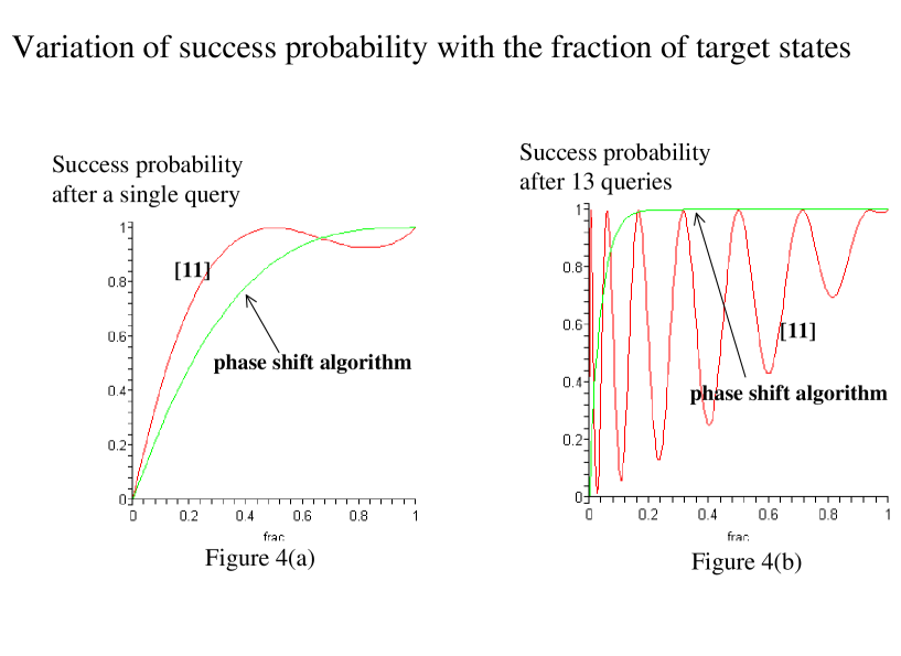
Figure 4: Comparison of the performance of the Phase-$\pi/3$ search algorithm with that of Ref.younes , when the fraction of marked states, $f$, varies between $0$ and $1$: (a) after one query, (b) after 13 queries.

How the quantum algorithms perform is graphically illustrated in Fig.4. For the particular distribution of $f$ considered above, Fig.4(a) shows that the graph of the fixed point search algorithm lies entirely above the graph of Ref. younes . The difference between the two becomes even more dramatic if we consider multiple query algorithms, as in Fig.4(b). As mentioned earlier, for the type of problems discussed in this section, the fixed point algorithm is the best possible quantum algorithm jai .

V Conclusion

The variant of quantum search discussed in this article supplements the original search algorithm, by providing a scheme that permits a fixed point and hence moves towards the target state in a directed way. The fixed point property makes the quantum search robust, and naturally leads to schemes for correction of systematic errors reichardt .

We have presented two implementations of the fixed point quantum search, both optimal in the worst-case scenario. At first sight, requirements of monotonic convergence and unitary quantum evolution appear to be in conflict. But the conflict has been avoided by a recursive approach in the Phase-$\pi/3$ search algorithm and by irreversible projections in the measurement based search algorithm. Between the two, the measurement based search algorithm is better behaved than the Phase-$\pi/3$ search, because (a) it allows all positive integer number of oracle queries instead of a restricted set of integers, and (b) its average-case requirement of number of oracle queries is smaller.

Deeper insights in to the mechanisms of these algorithms are still desirable. For instance, what is so special about phase shift of $\pi/3$, and how does the change of phase shift (from $\pi$ to $\pi/3$) convert the amplitude amplification algorithm to something totally different? Can one improve the algorithms in the non-asymptotic region by making the phase shifts (or rotation angles) a function of the query sequence, in a manner reminiscent of local adiabatic quantum algorithms? Such questions are definitely worth exploring.

The potential applications of these algorithms are in problems with small but unknown initial error probability and limited number of oracle queries, where they assure monotonic power-law convergence. For such problems, the fixed point algorithms are better than the best classical search algorithms by a factor of 2. Applications to pattern recognition and associative memory recall are under investigation.

References

- (1) G. Brassard, Searching a quantum phone book, Science 275 (1997) 627.
- (2) L.K. Grover, Quantum Mechanics helps in searching for a needle in a haystack, Phys. Rev. Lett. 78 (1997) 325.
- (3) G. Brassard, P. Hoyer, M. Mosca and A. Tapp, Quantum amplitude amplification and estimation, AMS Contemporary Mathematics Series Vol. 305, eds. S.J. Lomonaco and H.E. Brandt, (AMS, Providence, 2002), p.53, e-print quant-ph/0005055.
- (4) L.K. Grover, Quantum computers can search rapidly by using almost any transformation, Phys. Rev. Lett. 80 (1998) 4329.
- (5) L.K. Grover, Fixed-point quantum search, Phys. Rev. Lett. 95 (2005) 150501, e-print quant-ph/0503205.
- (6) T. Tulsi, L.K. Grover and A. Patel, A new algorithm for fixed point quantum search, Quant. Inform. and Comput. (2006), to appear, e-print quant-ph/0503205.
- (7) L.K. Grover, From Schrödinger’s equation to the quantum search algorithm, Pramana 56 (2001) 333, e-print quant-ph/0109116.
- (8) S. Chakraborty, J. Radhakrishnan and N. Raghunathan, Bounds for error reduction with few quantum queries, Proceedings of APPROX-RANDOM 2005, LNCS 3624 (Springer, Berlin, 2005), p.245.
- (9) C.H. Bennett, E. Bernstein, G. Brassard and U. Vazirani, Strengths and weaknesses of quantum computing, SIAM Journal on Computing 26 (1997) 1510.
- (10) C. Zalka, Grover’s quantum searching is optimal, Phys. Rev. A60 (1999) 2746.
- (11) A. Younes, J. Rowe, J. Miller, Quantum search algorithm with more reliable behavior using partial diffusion, quant-ph/0312022.
- (12) B.W. Reichardt and L.K. Grover, Quantum error correction of systematic errors using a quantum search framework, Phys. Rev. A72 (2005) 042326, e-print quant-ph/0506242.