Departament de Física
Universitat de les Illes Balears
Characterization of Quantum Entangled States and Information Measures
PhD Thesis

foreword

The present Thesis covers the subject of the characterization of entangled states by recourse to the so called entropic measures, as well as the description of entanglement related to several issues in quantum mechanics, such as the speed of a quantum evolution or the exciting connections existing between quantum entanglement and quantum phase transitions, that is, transitions that occur at zero temperature.

This work is divided in four parts, namely, I Introduction, II Quantum Entanglement, III The role of quantum entanglement in different physical scenarios, and IV Conclusions. At the end of it we include an Appendix with several historical remarks and technical details. The first introductory part consists in turn of three subsections: i) a historical review of what is undestood by Quantum Information Theory (QIT), ii) a brief description of quantum computation, and finally iii) an account on quantum communication. The first part dealing with the roots of information theory and its connection with physics has been included for the sake of completeness, mainly for historical reasons. One believes that a modern subject such as QIT, which is highly diverse and transverse, deserved a few lines so that the reader can realize the importance of the evolution towards the quantum domain of concepts such as (reversible) computability and the physical nature of information, as well as the analyses of fundamental arguments that questioned the completeness of the quantum theory, which in turn motivated and gave rise to the concept of quantum entanglement. The other two subsections on quantum computation and quantum communication are reviewed only because they offer brand new and exciting proposals, which are of common interest to any physicist. However, these former concepts are not present in the description of this Thesis, therefore one can skip them with no loss of continuity.

The second part entitled Quantum Entanglement describes the problem of detecting entanglement, added to the question of characterizing it. The third part covers the role of quantum entanglement in different contexts of quantum mechanics, and finally the Conclusions review some of the most important ideas exposed in the present work.

Part I Introduction

The characterization of quantum entangled states and their properties range from the description of quantum entanglement itself to the description of the states of quantum systems, where this quantum correlation can be present. The description of entangled states requires a two-step procedure: the i) detection of entanglement, combined with the ii) characterization of entanglement.

In the present Thesis we expose the tools employed in the characterization of bipartite quantum systems in multiple dimensions (e.g. $2\times 2$ or two-qubit systems, $2\times 3$, and so forth) by means of entropic or information measures. These information measures are described in forthcoming sections of this Introduction and more specifically in part II, entitled Quantum Entanglement, and also in the concomitant Chapters where this item is discussed in more detail. The relevance of this information-theoretical description resides in the fact that the entropic framework offers a highly intuitive and physical meaning to what entanglement represents in a bipartite quantum system: the entropy of any of its subsystems cannot be larger that the total entropy of the system. These relations, known as entropic inequalities, applied to the field of quantum information theory, constitute the subject of a novel study in this Thesis. Mathematically, it is a necessary condition for the discrimination of an entangled state: if a state does not possess quantum correlations, therefore it fulfils the entropic inequalities. However, the converse is not true, which means that one can encounter entangled states that look “classical”. By generating random mixed states of bipartite systems in different dimensions, we obtain the volume of states that comply with the entropic criteria, and compare it with several other criteria. Also in this Thesis, we reveal the interesting connection existing between a particular class of entangled states, the maximally entangled mixed states (MEMS), and the violation of the aforementioned entropic inequalities. However, previous to the detection of entanglement, in this Thesis we refute the fact that the maximum entropy principle applied to the inference of states “fakes” entanglement. That is, we show that a proper combination of maximization of entropy followed by minimization of entanglement leads to a correct description of the entanglement present in an inferred state, contrary to what was believed.

With respect to what implies the characterization of entangled states, we perform a Monte Carlo procedure in the exploration of the structure of the simplest quantum system that exhibits entanglement, the two-qubit system. Already in these systems, the space of mixed states to explore has got 15 dimensions and it is highly anisotropic. By generating mixed states of two qubit states according to different measures present in the literature, we can observe how entanglement is distributed in this space using the so called participation ratio –as sort of degree of mixture– as a probe. In clear connection with quantum computation, quantum gates acting on pure or mixed states act as entanglers: quantum gates represent the mathematical abstraction of a physical process of interaction. It has then been of interest to study how entanglement is distributed when a two-qubit gate acts on an arbitrary pure or mixed state.

Regarding the characterization of entanglement, first of all we review the measures of entanglement used to date. We point out that there exist obscure points in the current definition of entanglement, which is based in a preferred tensor product partition of the Hilbert space of the physical system under study. This is the starting point for employing a measure of entanglement introduced by the theoretical group of Los Alamos, the so called purity measure. This measure does not present problems when dealing with identical particles, nor with the total number of them. These features make it specially suitable for studying quantum entanglement in condensed matter systems. More specifically, here we describe the connection that exists between entanglement and quantum phase transitions, that is, transitions that occur at zero temperature. Our contribution, which is an extension of the work done at Los Alamos, deals with a more specific feature of quantum phase transitions, namely, their dynamics. We study the dynamical evolution of the $XY$ anisotropic model in a transverse magnetic field, which will reveal that entanglement can be regarded as a property that characterizes the overall system. Furthermore, we shall see that entanglement can present non-ergodic features, on equal footing with a clear physical magnitude such as the $z$-magnetization. In a different scenario, we also show that entanglement can speed up the evolution of a quantum state in a very special way: in general terms, an entangled state evolves to its first orthogonal faster than an unentangled one. This is also true for the extended usual measure of entanglement for indistinguishable particles only in the case of bosons, but not for fermions.

The present Thesis has been conceived to be read in a continuous way. In the Introduction (part I) we recall several ideas which are of basic nature if one wants to grasp the origins of a highly diverse subject such as quantum information theory, in an attempt to stress the fact that information has its roots not in abstract mathematical ideas, but in deep physical grounds. The tools employed and their description in the study of the characterization of entangled states are given in part II, while every Chapter of part III is almost self-contained: it exposes, when necessary, the tools that are needed in the description of entanglement in different contexts. The Conclusions (part IV) review the most important results obtained and a final Appendix contains technical details regarding procedures and concepts constantly referred to throughout the present contribution.

Chapter 1 Quantum information theory: a crossroads of different disciplines

Quantum information theory (QIT) is a fast developing science that has been built upon several branches of different scientific disciplines. The goals of QIT are at the intersection of those of quantum mechanics and information theory, while its tools combine those of these two theories. Behind what we call quantum information (it is yet unclear if quantum computation should be considered part of it, at least conceptually) one finds a whole spectrum of researchers working not only in the field of theoretical physics, but also mathematicians, computer scientists, electronic engineers, experimental physicists and so on. Of course all of them have different concerns and interests, and only in very recent years highly specialized conferences and meetings do offer a definite frame of reference for each one of these researchers. QIT finds room for theoretical physicists interested in the foundations of quantum mechanics (theory of measurement, quantum Zeno effect, decoherence, interpretation of quantum mechanics, Gleason’s Theorem, quantum jumps, etc..), Bell’s Theorem (Bell inequalities, Bell’s Theorem without inequalities, etc..), non-locality of Nature (local hidden variables theories, quantum entanglement and its description, separability, etc..), information processing (quantum cryptography, superdense coding, quantum teleportation, entanglement swapping, quantum repeaters, quantum key distribution, etc..); computer scientists and mathematicians (quantum computing, quantum algorithms, quantum complexity classes, etc..); both theoretical and experimental physicists (quantum circuits, quantum error correction, decoherence-free spaces, fault-tolerant quantum computation, nuclear magnetic resonance or NMR quantum computing, ion-trap quantum computing, optical lattice quantum computing, solid state quantum computing, etc..), and physicist interested in other related abstract features (quantum games, quantum random walks, etc..).

In spite of the clear diversity of interests, there exists a common feature that makes possible all previous challenges, which receives the name of entanglement. Until recent times, in relative terms, fundamental aspects of quantum theory were considered a matter of concern to epistemologists. While certainly profound questions were debated in the pursue of an answer of the ultimate nature of reality, it scarcely seemed possible that they could be answered by experiments. The EPR paradox posed by Einstein, Podolsky and Rosen (EPR) in 1935 [1] focused the attention of the physics community on the possible lack of completeness of the newborn quantum mechanics. In their famous paper they suggested a description of the world (called “local realism”) which assigns an independent and objective reality to the physical properties of the well separated subsystems of a compound system. Then EPR applied the criterion of local realism to predictions associated with an entangled state, a state that cannot be described solely in terms of the properties of its subsystems, to conclude that quantum mechanics is incomplete. EPR criticism was the source of many discussions concerning fundamental differences between quantum and classical description of nature. Schrödinger [2], regarding the EPR paradox, did not see a conflict with quantum mechanics. Instead, he defined that non-locality or “Verschränkung” (German word for entanglement) should be the characteristic feature of quantum mechanics. The link between Information Theory and entanglement was first considered by him, when he wrote that “Thus one disposes provisionally (until the entanglement is resolved by actual observation) of only a common description of the two in that space of higher dimension. This is the reason that knowledge of the individual systems can decline to the scantiest, even to zero, while that of the combined system remains continually maximal. Best possible knowledge of a whole does not include best possible knowledge of its parts – and that is what keeps coming back to haunt us” [2]. Schrödinger thus identified a profound non-classical relation between the information that an entangled state gives about the whole system and the corresponding information that is given to us about the subsystems. The most significant progress toward the resolution of this “academic” EPR problem was made by Bell [3, 4] in the 60s who proved that the local realism implies constraints on the predictions of spin correlations in the form of inequalities (called Bell’s inequalities) which can be violated by quantum mechanical predictions for the system. Experiments were carried out and confirmed Schrödinger’s argument (see forthcoming section on Bell inequalities for more details).

With time physicists have recognized the possibilities that entanglement, which is seen as a fundamental characteristic of Nature, can unfold at the technological stage, providing a new framework for developing faster computing (quantum computation) or impossible tasks in classical physics such as absolutely secure communication (quantum cryptography) or teleportation.

1.1 The roots of information theory and computer science

This section is devoted to the basic features of the origin of information theory and computer science. The motivation for doing so become clear as the theory of quantum information and computation borrow original ideas from these disciplines and translate them into the realm of quantum mechanics. Information in a technically defined sense was first introduced in statistics by R. A. Fisher in 1925 in his work on the theory of estimation. The properties of Fisher’s definition of information became a fundamental part of the so called statistical theory of estimation. Shannon and Wiener, indepently, published in 1948 works describing logarithmic measures of information for use in communication theory, which induced to consider information theory as synonymous with communication theory [5]. As a matter of fact, information theory formulates a communication system as a stochastic process. Formally, information theory is a branch of the mathematical theory of probability and mathematical statistics. As such, it can be applied in a wide variety of fields. Information theory is relevant to statistical inference, provides a unification of known results, and leads to natural generalizations [5]. In spirit and concepts, information theory has its mathematical roots in the concept of disorder or entropy in thermodynamics and statistical mechanics, as we shall see.

It is obvious that if one deals with a quantum information theory, it is because there exists a classical counterpart. As we shall see in future Chapters, quantum mechanics provide a framework where several mechanisms and concepts that appear in classical information are improved beyond what was thought to be an impossible barrier to overcome, while others simply did not exist. However, this is not so evident in the case of computer science. Historically, the first results in the mathematical theory of theoretical computer science appeared before the discipline of computer science existed; in fact, even before the existence of electronic computers. Shortly after Gödel proved his famous incompleteness theorem, there appeared several papers that drew a distinction between computable and non-computable functions. But of course one needed a mathematical definition of what was understood as “computable”, each author giving a different one. But in the end they all resulted in the same class of computable functions. This led to the proposal of what is known now as the Church-Turing thesis, named after Alonzo Church and Alan Turing. This thesis says that any function that is computable by any means, can be computed by a Turing machine. Once “computability” is defined, the task is to classify different problems into complexity classes. But this part will be explained in Chapter 2. The bridge existing between this discipline (computer science) and quantum information theory can only occur when the principles of quantum mechanics are observed. This will certainly take place in the near future, if it is not already the case, when the speed of computation will become limited by the quantum effects that appear in the miniaturization of the basic electronic devices (e.g. the basic logical gates). Only when one realizes that information is physical.., information processing, where computing is included, ought to obey the laws of quantum mechanics.

Therefore let us recall the origin of the basic concepts of information theory and computer science, so that we could gain more insight into the quantum counterpart.

1.1.1 Claude Shannon and the information measure $H$

In 1948 Shannon published A Mathematical Theory of Communication. This work focuses on the problem of how to best encode the information a sender wants to transmit. In this fundamental work he used tools in probability theory, which were in their nascent stages of being applied to communication theory at that time. His theory for the first time considered communication as a rigorously stated mathematical problem in statistics and gave communications engineers a way to determine the capacity of a communication channel in terms of the common currency of bits. The word “bit” is the short expression for “binary digit”, either 0 or 1, which is the abstract state one can assign to two possible outcomes in a binary system. Any text can be coded into a string of bits; for instance, it is enough to assign to each symbol its ASCII code number in binary form and append a parity check bit. For example, the word “quanta” can be coded as $11100010\,\,11101011\,\,11000011\,\,11011101\,\,11101000\,\,11000011$. Each bit can be stored physically; in classical computers, each bit is registered as a charge state of a capacitor (0=discharged,1=charged). They are distinguishable macroscopic states and rather robust or stable. They are not spoiled when they are read in (if carefully done) and they can be cloned or replicated without any problem. Information is not only stored; it is usually transmitted (communication) and sometimes processed (computation). With this description, we are just advancing some of the properties that ought to be carefully revisited in the quantum counterpart.

The transmission part of the theory is not concerned with the meaning (semantics) of the message conveyed, though the complementary wing of information theory concerns itself with content through lossy compression of messages subject to a fidelity criterion. Shannon developed information entropy as a measure for the uncertainty in a message while essentially inventing what became known as the dominant form of “information theory”. Shannon, advised by von Neumann, gave the name “entropy”

$$H\,=\,-\sum_{n=1}^{N}p_{n}\,{\rm log}_{2}\,p_{n}$$ (1.1)

to the information content of a given message. $p_{n}$ stands for the probability of the event $n$. Let us describe the situation somewhat in more detail. What Shannon conceived was the entropy (1.1) associated to a discrete random variable $X$ which could take $N$ possible values $\{x_{1},...,x_{N}\}$, with $p_{n}$ being the probability that $X$ takes the value $x_{n}$. $H$ can then be interpreted as a measure of ingorance or uncertainty associated to the probability distribution $\{p_{n}\}$. It is not about the knowledge about the distribution itself, but the capacity of predicting the results of an experiment subjected to this distribution. Thus, in his 1948 work, Shannon formalised the requirements of an information measure $H(p_{1},...,p_{N})$ with the following criteria:

• i) $H$ is a continuous function of the $\{p_{n}\}$.

• ii) If all probabilities are equal, $p_{n}=1/n$, then $H$ is a monotonic increasing function of $N$.

• iii) $H$ is objective, that is,

  $$H(p_{1},...,p_{N})\,=\,H(p_{1}+p_{2},p_{3},...,p_{N})\,+\,(p_{1}+p_{2})\,H\bigg{(}\frac{p_{1}}{p_{1}+p_{2}},\frac{p_{2}}{p_{1}+p_{2}}\bigg{)}.$$ (1.2)

This last condition entails that information does not change when one appropiately manages different chunks of it. The principle that entropy is a measure of our ignorance about a given physical system was recognized by Weaver, Shannon and Smoluchowski. Boltzmann was also aware of it. On the other hand, the mathematical theory of information originally was intended as a theory of communication, as we know. The simplest problem it deals with could be the following: given a message, one can represent it as a sequence of bits and thus, if the length of the “word” in $n$, one needs $n$ digits to characterize it. The set $E_{n}$ of all words of length $n$ contains $2^{n}$ elements, so the amount of information needed to characterize one element of its is log₂ of the number of elements of $E_{n}=$log${}_{2}N$, with $N=2^{n}$. Elaborating this argument a little bit more, one arrives at the result that the amount of information required to describe an element of any set of power $N$ is log${}_{2}N$. Now suppose that $E=E_{1}\cup...\cup E_{k}$ of pairwise disjoint sets, with $N_{i}$ representing the number of elements of $E_{i}$. Let $p_{i}=N_{i}/N$, $N=\sum_{i}N_{i}$. If one knows that an element of $E$ belongs to $E_{i}$, one needs log${}_{2}N_{i}$ additional information in order to determine it completely. Therefore the average amount of information needed to determine an element is $\sum_{i}(N_{i}/N)$log${}_{2}N_{i}$=$\sum_{i}p_{i}$log${}_{2}Np_{i}$=$\sum_{i}p_{i}$log${}_{2}p_{i}$+log${}_{2}N$. In consequence the lack of information is just -$\sum_{i}p_{i}$log${}_{2}p_{i}$, or just the entropy (1.1).

We do not discuss here the details of the measure $H$ here. They shall be discussed employing the von Neumann entropy $S(\rho)$. Also, the theorems related to information channels and data compression will be discussed when compared to the quantum case. However, we must point out that all possible candidates to become information measures or entropies have to follow the so called Khinchin axioms [7]. Two of them are convexity and additivity. By relaxing the convexity condition, one may encounter Rényi’s entropy, while relaxing the additivity constraint gives rise to Tsallis’ entropy. Both of them are parameterized with $q$ real, and recover the usual Shannon entropy (1.1) in the limit $q\rightarrow 1$. These features are described in detail in Chapters 4 and 7-9. The entropy $H$, when applied to an information source, could determine the capacity of the channel required to transmit the source as encoded binary digits. If the logarithm in the formula (1.1) is taken to base 2, then it gives a measure of entropy in bits. Shannon’s measure of entropy came to be taken as a measure of the information contained in a message, as opposed to the portion of the message that is strictly determined (hence predictable) by inherent structures, such as redundancy in the structure of languages or the statistical properties of a language relating to the frequencies of occurrence of different letter or words.

Information entropy as defined by Shannon and added upon by other physicists is closely related to thermodynamical entropy. A glance to (1.1) would tell any physicist that one is talking about entropy, but as we known, the word “entropy” is used in many contexts: information theory, thermodynamics, statistical mechanics, etc. Information, entropy, order and disorder are words that are often mixed altogether in the same context, adding more confusion. Of course there is a formal analogy of the information entropy (1.1) and Boltzmann-Gibbs’ $S=k\,$log$W$, which applies to microscopic systems. With the extension to quantum mechanics made by von Neumann, employing the density matrix formalism, one generalizes the concept of entropy to both classical and quantum physics. The final connection between information entropy and thermodynamical entropy is encountered by maximizing the former –restricted to several constrains– applied to the context of the latter, that is, the description of thermodynamics through the tools of statistical mechanics.

1.1.2 Jaynes’ principle and the thermodynamical connection: information and entropy

The similarities between the information entropy $H$ and Boltzmann’s entropy $S=k\,$log$W$, especially between the principle of maximum (informational) entropy (which adopts as we shall show an exponential form for the probability density distribution or the density matrix) and the Gibbs’ factor in statistical mechanics, were too much coincidence for E. T. Jaynes. To him, the principle of maximum entropy [8, 9], in the framework of inference of information, was advanced as the basis of statistical mechanics [10]. His idea was to view statistical mechanics as a form of inference: information theory provides a constructive criterion (the maximum-entropy estimate). If one considered statistical mechanics as a form of statistical inference rather than a physical theory, the usual rules were justified independently of any physical argument, and in particular independently of experimental verification. This was the gist of Jaynes’ principle.

According to Jaynes’ principle, one must choose the state yielding the least unbiased description of the system compatible with the available data. Either if we are dealing with classical or quantum statistical mechanics, the spirit is the same. That state is provided by the statistical operator $\hat{\rho}_{ME}$ that maximizes the von Neumann entropy $S\,=\,-Tr(\hat{\rho}\,\ln\hat{\rho})$ subject to the constraints imposed by normalization and the expectation values $\langle\hat{A}_{i}\rangle\,=\,Tr(\hat{\rho}\hat{A}_{i})$ of the relevant observables $\hat{A}_{i}$. The outcome of this procedure is a density matrix $\hat{\rho}$ proportional to $e^{-\sum_{i}\lambda_{i}\,\hat{A}_{i}}$, $\lambda_{i}$ being some suitable Lagrange multipliers.

What Jaynes’ prescription provides is the best “bet” that one can make on the basis of the available data. Clearly, this available information may not be enough to predict certain properties of the system. In such cases, Jaynes’ prescription is bound to “fail” because of a lack of input information [8, 9]. This point is the main subject of discussion in Chapter 1, in connection with the inference of states using MaxEnt procedures and entanglement.

Jaynes’ principle unties statistical mechanics from physical theories, and considers it as a suitable inference procedure. Certainly it is an interpretation of statistical mechanics in terms of an extremely simple inference scheme based of the expectation value of several observables, e.g. the system Hamiltonian $H$, hence the Gibbs’ factor $e^{-\beta\langle H\rangle}$, $\beta$ being a Lagrange multiplier. However, one still needs to associate or to interpret the concomitant Lagrange multiplier with definite physics quantities ($\beta\equiv 1/k_{B}T$).

Notice that by no means the aim of Jaynes’ principle is to justify the grounds of statistical mechanics. Aspects of the foundations of statistical mechanics [11] such as the $H$-Theorem or the Ergodic Theorem are questions out of the scope of these lines: Jaynes’ MaxEnt prescription cannot explain the fact that statistical mechanics has been able to predict accurately and successfully the behaviour of physical systems under equilibrium conditions. It rather simplifies instead the approach to statistical mechanics, and the proof of its success, the proof of the pudding, is in the eating.

1.1.3 Alan Turing and the universal computing machine

The birth of computer science is associated with the publication of the work “On Computable Numbers” by A. M. Turing in 1936, who is considered the father of computer science. He basically posed the operating principles (further developed by von Neumann in 1945) of ordinary computers (birth of the Turing machine). Together with A. Church they formulated what is known as the “Church-Turing hypothesis”: every physically reasonable model of computation can be efficiently simulated on a universal Turing machine [12].

A Turing machine is the mechanical translation of what a person does during a methodical process of reasoning. Turing also provided convincing arguments that the capabilities of such a machine would be enough to encompass everything that would amount to a recipe, which in modern language is what we call an algorithm. Turing arrived at this concept in his original paper [6] in an attempt to answer one of the Hilbert’s problem, namely, the problem of decidability: Does there exist a definite method by which all mathematical questions can be decided? In the Turing machine context, he found that the problem of determining whether a particular machine will halt on a particular input, or on all imputs, known as the Halting problem, was undecidable. Besides, the logicician A. Church shown that the decidability problem was unsolvable: there cannot be a general procedure to decide whether a given statement expresses an arithmetic truth. In other words, there will not be any Turing machine capable of deciding the truth of an arithmetic statement. In point of fact, undecidability shall lead in computer science to the classification of the types of problems that can be algorithmically solvable into a series of complexity classes. As we have seen, the birth of the Turing machine, of computer science, appeared in a context of a crisis in the foundations of mathematics.

Let us return to the concept of a Turing machine. More precisely, it consists of:

• A tape which is divided into cells, one next to the other. Each cell contains a symbol from some finite alphabet. This alphabet contains a special blank symbol (“0”) and one or more symbols. The tape is assumed to be arbitrarily extendible to the left and right. Cells have not been written before, containing the blank symbol.

• A head that can read and write symbols on the tape and move left and right.

• A state register that stores the state of the Turing machine. The number of different states is always finite. There exists a special start state which initializes the register.

• A transition function that tells the machine what symbol to write, how to move the head (“L” or “-1” for one step left, and “R” or “1” for one step right) and what its new state will be. If there is no entry in the function then the machine will halt.

According to the previous description, a Turing machine contains finite elements, except for the potentially unlimited amount of tape, which translates into unbounded capacity of storage space. More intuitively, a Turing machine can be viewed as an automaton that moves left-right and reads/writes on an infinite tape when it receives an order. More formally, a one-tape Turing machine is defined as a 6-tuple $M=(Q,A,\delta,s,F,b)$, where $Q$ is a finite set of states, $A$ is a finite set of the tape alphabet, $s\in Q$ is the initial state, $F\subseteq Q$ is the set of final or accepting states, $b\in A$ is the blank symbol (“0”) and $\delta$ is the transition function

$$\delta:\,Q\times A\,\rightarrow\,Q\times A\times\{-1,0,1\}.$$ (1.3)

Extensions to $k$-tape Turing machines are straightforward. What changes is the definition in the transition function

$$\delta:\,Q\times A^{k}\,\rightarrow\,Q\times\big{(}A\times\{-1,0,1\}\big{)}^{k}.$$ (1.4)

The previous definitions for Turing machines on one tape or several tapes belong to the class of deterministic Turing machines (when the transition function has at most one entry for each combination of symbol and state). Turing machines are useful models of real (classical) computers. Despite their simplicity, Turing machines can be devised to compute remarkably complicated functions. In fact, a Turing machine can compute anything that the most powerful ordinary classical computer can compute, which boils down to the aforementioned Church-Turing hypothesis. Why universal Turing machines? The importance of the universal machine is clear. We do not need to have an infinity of different machines doing different jobs. A single one will suffice. The engineering problem of producing various machines for various jobs is replaced by the office work of programming the universal machine to do these jobs. In summary, a Turing machine is comparable to an algorithm much as the universal Turing machine is to a programmable computer [12].

Now, there also exist a model for probabilistic Turing machines, that is more suitable in order to tackle a generalization to the quantum domain. Defining the same a 6-tuple $M=(Q,A,\delta,s,F,b)$, the new transition function becomes a transition probability distribution

$$\delta:\,Q\times A\,\times Q\times A\,\times\{-1,0,1\}\,\rightarrow\,[0,1].$$ (1.5)

The value $\delta(q_{1},a_{1},q_{2},a_{2},d)$ has to be viewed as the probability that when the machine is in state $q_{1}$ and reads the symbol $a_{1}$, it will write the symbol $a_{2}$, jump to the state $q_{2}$ and move the head to the direction $d\in\{-1,0,1\}$. Clearly, it is required that for all initial states $(q_{1},a_{1})\in Q\times A$

$$\sum_{{\rm All\,possible\,final\,states}\,(q_{2},a_{2})}\delta(q_{1},a_{1},q_{2},a_{2},d)\,=\,1.$$ (1.6)

Although the basics of quantum computation will be exposed in Chapter 2, let us show how a quantum Turing machine would look like. In the same vein as before, the 6-tuple $M=(Q,A,\delta,s,F,b)$ is formally the same, although the “states” have to be considered quantically, and we replace probabilities with transition amplitudes. Therefore we have a transition amplitude function

$$\delta:\,Q\times A\,\times Q\times A\,\times\{-1,0,1\}\,\rightarrow\,\mathcal{C}$$ (1.7)

that generalizes the probabilistic Turing machine 1.5. $\delta(q_{1},a_{1},q_{2},a_{2},d)$ are now complex amplitudes, that satisfy the normalization condition

$$\sum_{{\rm All\,possible\,final\,states}\,(q_{2},a_{2})}|\delta(q_{1},a_{1},q_{2},a_{2},d)|^{2}\,=\,1.$$ (1.8)

A quantum Turing machine operates in steps of fixed duration $T$, and during each step only the processor and a finite part of the memory unit interact via the cursor. We stress that a quantum Turing machine, much like a Turing machine, is a mathematical construction [12]; we shall present explicit experimental realizations of equivalent quantum circuits (see Chapter 2). The state of the computation is the state of the whole quantum Turing machine (Hilbert space $\cal{H}_{QC}$), represented by $|\Psi\rangle$. All the set of instructions are encoded in the unitary time evolution $U$ of state $|\Psi\rangle$, such that after a number $n$ of computational steps, the state of the system has evolved to $|\Psi(n\,T)\rangle=U^{n}\,|\Psi(0)\rangle$.

Because of unitarity, the dynamics of a quantum computer, as in the case of any closed quantum system, are necessary reversible. Turing machines, on the one hand, undergo irreversible changes during computations and until the 80s it was widely held that irreversibility was an essential feature of computation. Turing machines, like other computers, often throw away information about their past, by making a transition into a logical state whose predecessor is undefined. However, Bennett [13] proved in 1973 that this should not be the case by constructing explicitly a reversible classical model computing machine equivalent to Turing’s. This so called “logically” irreversibility has an important bearing on the issue of thermodynamics of (classical) computation, which is the subject of the next section.

Summing up, Turing’s invention was built on the insight of Kurt Gödel that both numbers and operations on numbers can be treated as symbols in a syntactic sense. The way to modern (classical) computers starts with the definition of a Turing machine, followed by the basic Boolean operations carried out by logic gates inserted in integrated circuits. Nowadays we take for granted that all information and programming instructions can be expressed by strings of 0 and 1, and that all computations, ranging from simple arithmetic operations to proving theorems, can be carried out when a set of systematic operations (the program) are applied to this string of bits. However, we do not discuss here the technical part that deals with actual (classical) computing. Instead, it shall be revisited in the description of the quantum counterpart.

1.1.4 Thermodynamics of information and classical computation

“The digital computer may be thought of as an engine that dissipates energy in order to perform mathematical work.”
C. H. Bennett in [14].

While I am writing these lines, I can perfectly hear the swing of the laptop. And if I place my hand behind it, I shall notice the flow of hot air. This fact simply means that my computer (and any classical computer known to date) dissipates energy in the form of heat. Although modern computers are several orders of magnitude more efficient (energetically) than the first electronic ones, they still release vast amounts of energy as compared with $k_{B}\,T$. Even in the hypothetical case where perfectly engineered classical computers should not have to be cooled down in order to perform basic operations, we would end up with a physical thermodynamical minimum limit of heat released during calculations. This is due to the fact that information is not always stored; most of the time a lot of useless information is erased. According to Landauer [15], an irreversible overwriting of a bit causes at least $k_{B}T$ln2 Joules of heat being dissipated. In other words, erasure of a bit of information in an environment at temperature $T$ leads to a dissipation of energy no smaller than $k_{B}T$ln2.

Why is this so? In a sense, everything dates back to the 19th century, before quantum mechanics or information theory were conceived. Maxwell found in his famous paradox an apparent contradiction with the Second Law of thermodynamics. Maxwell considered an intelligent being (which could be a programmed machine), later baptized as a Demon, which was able to open and close a gate inside a gas vessel, which is divided into two parts. By letting faster molecules pass through the gate only, this Demon would increase the temperature of one side of the vessel without work, thus violating the Second Law. It was Szilard [16] who refined in 1929 the conceptual model proposed by Maxwell into what is now known as Szilard’s engine. This is a box with movable pistons at either end, and a removable partition in the middle. The walls are maintained at constant temperature $T$, and a particle collides with the walls. A cycle of the engine begins with the Demon partitioning the box and observing which side the particle is on. It then moves the piston towards the empty side up to the partition, removes the partition, and allows the particle to push the piston back to its starting position, the whole cycle being isothermal. At each cycle the engine supplies $k_{B}T$ln2, violating the Second Law. Szilard deduced that, if we do not want to admit that the Second Law has been violated, the intervention which establishes the coupling between the measuring apparatus and the thermodynamic system must be accompanied by a production of entropy, and he gave the explicit form of the “fundamental amount” $k_{B}$ln2, which is the entropy associated to a dichotomic or binary decision process. In other words, the entropy of the Demon must increase, conjecturing that this would be a result of the (assumed irreversible) measurement process. Szilard not only defined the quantity that it is known today as information, which found vast applications with the work of Shannon, but also finds the physical connection between thermodynamic entropy and information entropy when he establishes that one has to pay (at least) $k_{B}T$ln2 units of free energy per bit of information gain. Szilard’s argument was a pioneering insight of the physical nature of information, indeed. Later on, von Neumann also associated entropy decrease with the Demon’s knowledge in his 1932 Mathematische Grundlagen der Quantenmechanik [17].

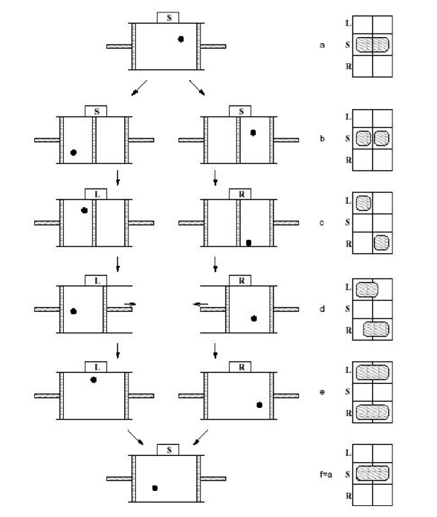
Figure 1.1: A one molecule Maxwell’s Demon apparatus (after [14]). On the right there is a phase diagram with the Demon’s coordinates on the vertical axis.

The resolution of the paradox would lead to the discovery of a connection between physics and the gathering of information. The Demon was finally exorcised in 1982 by Bennett [14]. In the meantime, in order to rescue the Second Law, many efforts were made involving analyses of the measurement process, such as information acquisition via light signals (L. Brillouin in [18]), which were temporary resolutions. Bennett observed that the Demon “remembers” the information it obtains, much as a computer records data in its memory. He then argued that erasure of Demon’s memory (and here is the link with Landauer’s work on computation) is the fundamental act that saves the Second Law. Let us follow Bennett’s argument with the help of Fig.1.1, taken from [14], and follow the phase space changes of Demon’s coordinates through one cycle. In (a) the Demon is in a standard state and the particle is anywhere in the box. In (b) the partition is inserted and in (c) the Demon makes his measurement. By doing so, his state of mind becomes correlated with the state of the particle. Note that the overall entropy has not changed. Isothermal expansion takes place in (e), and the entropy of the particle plus the Demon increases. After expansion the Demon remembers some information, but this is not correlated to the particle’s position. In the way back to his standard state in (f) we increase its entropy, dissipating energy into the environment. If von Neumann had addressed in 1932 the process of discarding information in order to bring back the Demon to its initial state, he might have discovered what Bennett solved a lot earlier.

Returning to the heat release due to erasure of information, Bennett [13] also proved that reversible computation, which avoids erasure of information, which in turn is tantamount as avoiding an energy release, was possible in principle. Bennett’s construction of a reversible Turing machine uses in fact three tape Turing machines: input tape, history tape and output tape. When we simulate the original machine in the input tape, we store the transition rules in the history tape. In this way we obtain reversibility. Every time the machine stops, we copy the output from the input tape to the output tape, which is empty. Then we compute backwards in order to erase the history time for further use. Although we do not give the details, this construction consumes considerable memory, being reduced by erasing the history tape recursively, has got constant slowdown and increases the space consumed. Nevertheless, Bennett thus established that whatever is computable with a Turing machine, it is also computable with a reversible Turing machine.

Maxwell’s demon revisited: information and measurement in the light of quantum mechanics

Until the work of Bennett in 1973 [13], it was thought that the computation process was necessarily irreversible, where energy dissipation was associated with information erasure. However he showed that to every irreversible computation there exists an equivalent reversible computation. But Bennett’s work did not addressed concerns realted to quantum effects. Certainly processes such as “measuring” had to be carefully studied in the quantum domain.

It was Zurek [19] who careful performed a quantum analysis of Szilard’s engine. He considered a particle in an infinite square well potential, with the following dimensions: lenght $L$, the classical piston replaced by a finite barrier of length $\delta<<L$ and height $U>>k_{B}T$, which is slowly inserted. In the quantum version, Zurek shows that the validity of the Second Law is satisfied only if the measurement induces an increase of the entropy of the measuring apparatus by an amount which has to be greater or equal to the amount of information gained [19]. Zurek arrives to this main result by observing that the system can at all times be described by its partition function. This means that the thermodynamic approximation is indeed valid. A quantum Demon explicitly has to reset itself, thus demonstrating that Bennett’s conclusion regarding the destination of the excess entropy is also correct. The measurement of the location of the molecule was of essential nature in the process of extracting work in both classical and quantum versions of Szilard’s engine.

The fact that erasure of information is a process which costs free energy has interesting echoes in quantum information theory. To be more precise, if one is able to efficiently erase information, which is tantamount as to saturate Landauer’s bound $k_{B}T$ln2, then one can provide a physical interpretation [20, 21] of the so called Holevo bound [22], which is related to the information capacity in quantum channels (Chapter 3). It is interesting to see that a bound that is found as a relation satisfied by the von Neumann entropy can be interpreted in terms of Landauer’s bound $k_{B}T$ln2.

1.2 Foundational and fundamental aspects of quantum mechanics

“I think I can safely say that nobody today understands quantum mechanics.”
R. P. Feynman in [23].

Quantum physics was born in 1900 on Max Planck’s hypothesis of discretized energy packets or quanta –hence the name quantum– as a working hypothesis in order to explain the spectrum of a black body, which put an end to the classical period. But it was Einstein in 1905 who became the first physicist to apply Max Planck’s quantum hypothesis to light (explanation of the photoelectric effect). Einstein realized that the quantum picture can be used to describe the photoelectric effect. Later on they followed the quantization of the energy levels of atoms by Bohr (1913), the famous Stern-Gerlach experiment (1922) describing the quantization of the atomic systems, the de Broglie hypothesis of particles behaving as waves (1924), the first interference experiments with electrons carried out by C. J. Davidson and L. H. Germer (1927), and the confirmation of the photon theory with the Compton effect (1924). The Bohr correspondence principle formulated in 1923, namely, Quantum Theory must approach Classical Theory assymptotically in the limit of large quantum numbers and the subsequent Bohr-Sommerfeld quantization rules close the period known as Old Quantum Theory. Although the Old Theory undoubtly represented a great step forward, predicting a considerable body of experiments from simple rules, it was a rather haphazard mixture of classical mechanics and ad hoc prescriptions.

The physical theory of quantum mechanics (QM) was born by the efforts of men such as M. Born, P. A. M. Dirac, P. Jordan, W. Pauli, E. Schrödinger and W. Heisenberg. The founding of QM can be placed between 1923 and 1927 and put an end to the ambiguities of the Old Theory. Thereof matrix mechanics and wave mechanics have been proposed almost simultaneously: Schrödinger’s wave formulation and Heisenberg’s matrix formulation were shown to be equivalent mathematical constructions of QM. The transformation theory invented by Dirac unified and generalized Schrödinger’s and Heisenberg’s matrix formulation of QM. In this formulation, the state of the quantum system encodes the probabilities of its measurable properties or “observables”, which is a technical word in QM with a definite meaning. Roughly speaking, QM does not assign definite values to observables. Instead, it makes predictions about probability distributions of the possible outcomes from measuring an observable.

The problem about quantum mechanics does not lie on its effectivity, but on its interpretation. Any attempt to interpret quantum mechanics tries to provide a definite meaning to issues such as realism, completeness, local realism and determinism. Historically, the understanding of the mathematical structure of QM went trough various stages. At first, Schrödinger did not understand the probabilistic nature of the wavefunction of the electron. It was Born who proposed the widely accepted interpretation as a probability distribution in real space. Also, Einstein had great difficulty in coming to terms with QM (section on EPR paradox). Nowadays the Copenhagen interpretation (after Bohr and Heisenberg) of QM is the most widely-accepted one, followed by Everett’s many worlds interpretation [26]. Very briefly, the Copenhagen assumes two processes influencing the wavefunction, namely, i) its unitary evolution according to the Schrödinger equation, and ii) the process of measurement. As it is well known, the Copenhagen interpretation postulates that every measurement induces a discontinuous break in the unitary time evolution of the state through the collapse of the total wave function onto one of its terms in the state vector expansion (uniquely determined by the eigenbasis of the measured observable), which selects a single term in the superposition as representing the outcome. The nature of the collapse is not at all explained, and thus the definition of measurement remains unclear. Macroscopic superpositions are not a priori forbidden, but never observed since any observation would entail a measurementlike interaction. In the words of philosophy, Bohr followed the tenets of positivism, that implies that only measurable questions should be discussed by scientists.

Some physicists (see Ref. [27]) argue that an interpretation is nothing more than a formal equivalence between a given set of rules for processing experimental data, thus suggesting that the whole exercise of interpretation is unnecessary. It seems that a general consensus has not yet been reached. In the opinion of Roger Penrose [28], who remarks that while the theory agrees incredibly well with experiment and while it is of profound mathematical beauty, it “makes absolute no sense”.

The present status of quantum mechanics is a rather complicated and discussed subject (see Ref. [29, 30]). The point of view of most physicist is rather pragmatic: it is a physical theory with a definite mathematical background which finds excellent agreement with experiment. In this Chapter we shall present the most important results regarding Quantum Mechanics and several issues in quantum information theory. We shall not discuss the philosophical implications of results such as the interpretation of QM (completely out of the scope of this Thesis) which, since the advent of quantum entanglement, has gain considerable attention among the physics community.

1.2.1 The postulates of quantum mechanics

In this seccion we are going to provide a brief review of the basic formalism of quantum mechanics and of its Postulates. Here we closely follow the definitions given by C. Cohen et al. in [31].

In the mathematical rigorous formulation of quantum mechanics [32], developed by P. A. M. Dirac and J. von Neumann, the possible states of a quantum system are represented by “state vectors” (unit vectors) living in a complex Hilbert space, usually known in the quantum theory jargon as the “associated Hilbert space” of the system. Observables are represented by an Hermitian (or self-adjoint) linear operator acting on the state space. Each eigenvector of the operator possesses an eigenstate of an observable, which corresponds to the value of the observable in that eigenstate. The operator’s spectrum can be discrete or continuous. The fundamental role played by complex numbers in quantum theory has been found very intriguing by some physicists. Attemps to reach a deeper understanding of this aspect of quantum theory have led some researchers to consider a quantum formalism based upon quaternions [33]. However, it seems that the field of complex numbers is enough in order to describe quantum phenomena.

The time evolution (time $t$ is not an observable in quantum mechanics) of a state is determined by the Schrödinger equation, in which the Hamiltonian $H$, through a unitary matrix obtained by complex-exponentiating $H$ times $t$, generates the time evolution of that state. The modulus of it describes the evolution of a probability distribution, while the phase provides information about interference, hence the name wavefunction as being synonymous with quantum state. Schrödinger’s equation is completely deterministic, so there is nothing new in this sense as compared with classical mechanics.

Heisenberg uncertainty principle is represented by the fact that two observables do not commute. Using Max Born’s interpretation, the inner product between two states is a probability amplitude (usually a complex number). The possible outcomes of a measurement are the eigenvalues of the operator –this explains why observables have to be hermitian, i.e., they must be real numbers. The process of measurement is not yet understood (it is non-unitary): the system collapses from the initial state to one of its eigenstates with a probability given by the square of their inner product.

One can also look at quantum mechanics using Feynman’s path integral formulation, which is the quantum-mechanical counterpart of the least action principle in classical physics.

Postulate 1

“The state of a system is described by a vector in a Hilbert space ${\cal H}$”.

The state of any physical system at time $t$ is defined by specifying a ket $|\psi(t)\rangle$ belonging to a state space ${\cal H}$. ${\cal H}$ is a vector space, with the concomitant property of linearity. A Hilbert space is complex vector space with a scalar product.

Postulate 2 (principle of spectral decomposition)

“a) Discrete spectrum

The probability that a measurement of an observable $\hat{A}$ yields an eigenvalue $a_{n}$ when the system is in a normalized state $|\psi\rangle$ is given by

$$P(a_{n})=\sum_{i=1}^{g_{n}}|\langle a_{n}^{(i)}|\psi\rangle|^{2},$$ (1.9)

where $|a_{n}^{(i)}\rangle$ is a normalized eigenvector of $\hat{A}$ associated with $a_{n}$, and $g_{n}$ is its degeneracy.

b) Continuous non-degenerate spectrum

The probability that a measurement of an observable $\hat{A}$ yields a value between $\alpha$ and $\alpha$+$d\alpha$ when the system is in a normalized state $|\psi\rangle$ is given by

$$dP(\alpha)=|\langle\alpha|\psi\rangle|^{2}\,d\alpha,$$ (1.10)

where $|\alpha\rangle$ is the eigenvector of $\hat{A}$ associated with the eigenvalue $\alpha$”.

Postulate 3

“Physical observables are represented by hermitian operators that act on ket vectors”.

The results of a measurement is given by the eigenvalues of the operator $\hat{O}$. By the spectral decomposition principle we can write this operator as

$$\hat{O}=\sum_{i}o_{i}|W_{o_{i}}\rangle\langle W_{o_{i}}|,$$ (1.11)

where $|W_{o_{i}}\rangle$ are the eigenstates of $\hat{O}$.

One way of defining a state using an hermitian operator is possible through the definition of the density matrix $\rho$. If the system is found in a pure state $|\psi\rangle$, then $\rho=|\psi\rangle\langle\psi|$. Due to interaction with the environment, the state of the system is usually found in a admixture of states $\rho=\sum_{i}\lambda_{i}|\psi_{i}\rangle\langle\psi_{i}|$, with $0\leq\lambda_{i}\leq 1$. It has the properties i) Tr($\rho$)=1 and ii) being positive for all states $|\phi\rangle$, that is, $\langle\phi|\rho|\phi\rangle\geq 0$, where $\rho$ is an hermitian operator, but not an observable. The state $\rho$ contains all the information that can be accessed about the system.

Postulate 4 (reduction postulate, i.e, collapse of the wavefunction)

“The action of a measurement is to project the state into an eigenstate of the observable $\hat{O}$”.

Given an eigenvalue $o$ of the observable $\hat{O}$, the projector $P_{o}$ onto the subspace expanded by the eigenstates with eigenvalue $o$ is $P_{o}=\sum_{o_{i}=o}|\Psi_{o_{i}}\rangle\langle\Psi_{o_{i}}|$, where the sum runs over all the eigenvectors sharing the same eigenvalue $o$. After the measurement, the state is given by

$$|\Psi_{o_{i}}\rangle=\frac{\hat{P}_{o_{i}}|\Psi\rangle}{\sqrt{\langle\Psi|\hat{P}_{o_{i}}|\Psi\rangle}}.$$ (1.12)

In terms of the density matrix, we have

$$\rho\prime=|\Psi_{o_{i}}\rangle\langle\Psi_{o_{i}}|=\frac{\hat{P}_{o_{i}}\hat{\rho}\hat{P}_{o_{i}}^{\dagger}}{Tr(\hat{\rho}\hat{P}_{o_{i}})},$$ (1.13)

with the assumptions of i) orthogonality Tr($\hat{P}_{o_{i}}\hat{P}_{o_{j}}^{\dagger}=\delta_{i,j}$) and ii) closure $\sum_{i}\hat{P}_{o_{i}}=\hat{I}$.

There is a generalization of the concept of measurement to POVM (positive operator-valued measure) where the different measurements are not orthogonal (i.e. they are represented by operators $\hat{A}$,$\hat{B}$ such that Tr($\hat{A}\hat{B}$)$\neq 0$). The previous measurement is known as a von Neumann or projective measurement [34].

Postulate 5

“The evolution of an isolated quantum system is given by the Schrödinger equation

$$i\,\hbar\,\frac{\partial}{\partial t}\,|\psi(t)\rangle\,=\,\hat{H}\,|\psi(t)\rangle$$ (1.14)

where $\hat{H}$ is the Hamiltonian of the system, the operator related to the total energy”.

There is a formal solution to (1.14) given by $|\psi(t)\rangle=\exp(-\frac{i}{\hbar}\int dt\,\hat{H})|\psi(0)\rangle$. Because $\hat{H}$ is hermitian, $U\equiv\exp(-\frac{i}{\hbar}\int dt\,\hat{H})$ is a unitary operator. In quantum computation, $U$ is the representation of an algorithm.

As a final remark, we could postulate also that the state space of a composite physical system is given by the tensor product of the state space of its components, as opposed to the cartesian product in classical physics. Directly linked to the tensor product nature of state space, it emerges the notion of reduced matrices , which in a composite systems are used in order to address individual subsystems.

1.2.2 The EPR paradox: non-locality and hidden variable theories

Einstein never liked the implications of quantum theory, despite the undeniable success of quantum theory. Einstein’s hope was that quantum mechanics could be completed by adding various as-yet-undiscovered variables. These “hidden” variables, in his opinion, would let us regain a deterministic description of nature. The completeness of quantum mechanics was attacked by the Einstein-Podolsky-Rosen gedanken experiment [1] which was intended to show that there have to be hidden variables in order to avoid non-local, instantaneous “effects at a distance”. In the original paper, the position-momentum uncertainty relation served as a guideline for their argument, although it is most clear to us with the help of D. Bohm [36] employing a pair of spin-$\frac{1}{2}$ particles in a singlet state.

In their paper, EPR argued that any description of nature should obey the following two properties:

• Anything that happens here and now can influence the result of a measurement elsewhere, but only if enough time has elapsed for a signal to get there without travelling faster than the speed of light.

• The result of any measurement is predetermined. In other words a result is fixed even if we do not carry out the measurement itself.

EPR then studied what consequences these two conditions would have on observations of quantum particles that had previously interacted with one another. The conclusion was that such particles would have very peculiar properties. In particular, the particles would exhibit correlations that lead to contradictions with Heisenberg’s uncertainty principle. Their conclusion was that quantum mechanics was an incomplete theory.

The relevance of the EPR paradox was that it motivated a debate in the physics community, with the celebrated Schrödinger’s reply [2] introducing entanglement as the characteristic feature of quantum mechanics. As we shall see, thirty years later J. Bell [3, 4] tried to find a way of showing that the notion of hidden variables could remove the randomness of quantum mechanics. For more than three decades, the EPR paradox (or how to make sense of the (presumably) non-local effect one particle’s measurement has on another) was nothing more than a philosophical debate for many physicists. Bell’s theorem concluded that it is impossible to mimic quantum theory with the help of a set of local hidden variables. Consequently any classical imitation of quantum mechanics ought to be non-local. But this fact does not imply [37] the existence of any non-locality in quantum theory itself.

1.2.3 Testing Nature: John Bell’s inequalities

According to quantum mechanics, the properties of objects are not sharp. They are well defined only after measurement. Given two quantum particles that have interacted with each other, the possibility of predicting properties without measurement on either side led to the EPR paradox. The postulation of unknown random variables, “hidden” variables, would restore localism. On the other hand, randomness is intrinsic to quantum mechanics.

Bell devised an experiment that would prove it properties are well-defined or not, an experiment that would give one result if quantum mechanics is correct and another result if hidden variables are needed. Although the concomitant theorem is named after John Bell, a number of different inequalities have been derived by different authors all termed “Bell inequalities”, and they all purport to make the same assumptions about local realism. The most important are Bell’s original inequality [3, 4], and the Clauser-Horne-Shimony-Holt (CHSH) inequality [39]. Let us recall the original Bell’s invitation to his enterprise .

“Theoretical physicists live in a classical world, looking out into a quantum-mechanical world. The latter we describe only subjectively, in terms of procedures and results in our classical domain. (…) Now nobody knows just where the boundary between the classical and the quantum domain is situated. (…) More plausible to me is that we will find that there is no boundary. The wave functions would prove to be a provisional or incomplete description of the quantum-mechanical part. It is this possibility, of a homogeneous account of the world, which is for me the chief motivation of the study of the so-called “hidden variable” possibility.

(…) A second motivation is connected with the statistical character of quantum-mechanical predictions. Once the incompleteness of the wave function description is suspected, it can be conjectured that random statistical fluctuations are determined by the extra “hidden” variables – “hidden” because at this stage we can only conjecture their existence and certainly cannot control them.

(…) A third motivation is in the peculiar character of some quantum-mechanical predictions, which seem almost to cry out for a hidden variable interpretation. This is the famous argument of Einstein, Podolsky and Rosen. (…) We will find, in fact, that no local deterministic hidden-variable theory can reproduce all the experimental predictions of quantum mechanics. This opens the possibility of bringing the question into the experimental domain, by trying to approximate as well as possible the idealized situations in which local hidden variables and quantum mechanics cannot agree.”

Let us follow the development of the Bell’s original inequality. With the example advocated by Bohm and Aharonov [36], the EPR argument is the following. Let us consider a pair of spin one-half particles in a singlet state, and we place Stern-Gerlach magnets in order to measure selected components of the spins ${\bf\sigma}_{1}$ and ${\bf\sigma}_{2}$. If the measurement of the component ${\bf\sigma}_{1}\cdot{\bf a}$, with ${\bf a}$ being some unit vector (observable ${\bf a}$) , yields $+1$, then the quantum mechanics says that measurement of the component ${\bf\sigma}_{2}\cdot{\bf a}$ must yield $-1$, and vice versa. This is so because the two particles are anticorrelated. It is plain that one can predict in advance the result of measuring any chosen component of ${\bf\sigma}_{2}$, by previously measuring the same component of ${\bf\sigma}_{1}$.

Now let us construct a classical description of these correlations. Let us suppose that there exist a continuous hidden variable $\lambda$. The corresponding outcomes of measuring ${\bf\sigma}_{1}\cdot{\bf a}$ and ${\bf\sigma}_{2}\cdot{\bf b}$ are $A({\bf a},\lambda)=\pm 1$ and $B({\bf b},\lambda)=\pm 1$, respectively. The key ingredient is that result $B$ for particle 2 is independent of the setting ${\bf a}$, nor $A$ on ${\bf b}$, in other words, we address individual particles locally. Suppose that $\rho(\lambda)$ is the probability distribution of $\lambda$ (with $\int d\lambda\rho(\lambda)=1$). If the quantum-mechanical expectation value of the product of the two components ${\bf\sigma}_{1}\cdot{\bf a}$ and ${\bf\sigma}_{2}\cdot{\bf b}$ is

$$\langle\,{\bf\sigma}_{1}\cdot{\bf a}\,{\bf\sigma}_{2}\cdot{\bf b}\,\rangle\,=\,-\,{\bf a}\cdot{\bf b},$$ (1.15)

then the hidden variable model would lead to

$$P({\bf a},{\bf b})\,=\,\int d\lambda\,\rho(\lambda)\,A({\bf a},\lambda)B({\bf b},\lambda).$$ (1.16)

If the hidden variable description has to be correct, then result (1.16) must be equal to (1.15). Now let us impose anticorrelation in this scheme: $A({\bf a},\lambda)=-B({\bf a},\lambda)$ and (1.16) now reads

$$P({\bf a},{\bf b})\,=\,-\int d\lambda\,\rho(\lambda)\,A({\bf a},\lambda)A({\bf b},\lambda).$$ (1.17)

Adding one more unit vector ${\bf c}$, we have

$$P({\bf a},{\bf b})\,-\,P({\bf a},{\bf c})\, = \,-\int d\lambda\,\rho(\lambda)\,[A({\bf a},\lambda)A({\bf b},\lambda)-A({\bf a},\lambda)A({\bf c},\lambda)]$$ (1.18)

$$= \,\int d\lambda\,\rho(\lambda)\,A({\bf a},\lambda)A({\bf b},\lambda)[A({\bf a},\lambda)A({\bf c},\lambda)\,-\,1].$$ (1.19)

Bearing in mind that $A({\bf a},\lambda)=\pm 1$ and $B({\bf b},\lambda)=\pm 1$, (1.18) now reads

$$|P({\bf a},{\bf b})\,-\,P({\bf a},{\bf c})|\,\leq\,\int d\lambda\,\rho(\lambda)\,[1\,-\,A({\bf b},\lambda)A({\bf c},\lambda)]\,=\,1\,+\,P({\bf b},{\bf c}).$$ (1.20)

In a more compact fashion, Bell’s original inequality reads

$$1\,+\,P({\bf b},{\bf c})\,\geq\,|P({\bf a},{\bf b})\,-\,P({\bf a},{\bf c})|.$$ (1.21)

If we manage to perform an experiment that violates this inequality, the local hidden variables theories are not valid. In the case of a singlet state $|\psi\rangle=1/\sqrt{2}\,(|01\rangle-|10\rangle)$, the quantum mechanical prediction (1.15) is equal to $-\rm{cos}({\bf a},{\bf b})$, which violates Bell’s inequality (1.21) for several ranges of angles.

In the case of the CHSH inequality [39], we can relax the conditions $A({\bf a},\lambda)=\pm 1$ and $B({\bf b},\lambda)=\pm 1$ to $|A({\bf a},\lambda)|\leq 1$ and $|B({\bf b},\lambda)|\leq 1$. Proceeding as before, we thus arrive to

$$|P({\bf a},{\bf b})\,-\,P({\bf a},{\bf d})|\,+\,|P({\bf c},{\bf d})\,-\,P({\bf c},{\bf b})|\,\leq\,2.$$ (1.22)

The quantum limit of the CHSH inequality (1.22), that is, the right hand side of the inequality is larger by a factor of $\sqrt{2}$.

As suggested by Bell, these inequalities can be tested experimentally [40], using coincidence counts. Pairs of particles are emitted as a result of a quantum process, and further analysed and detected. In practice, to have perfect anticorrelation is difficult to obtain. Moreover, the system is always coupled to an environment. Although several experiments validate the quantum-mechanical view, the issue is not conclusively settled. Thanks to the high quality of the crystals used for parametric down conversion it is now possible to observe entangled particles that are separated by a distance of almost 10 km. None of these experiments supports the need for hidden variables, although we cannot be totally sure because they do not detect a big enough fraction of the total flux of photons (detection loopholes). An experiment that has no loopholes has not yet been performed [41]. The ultimate experimental test would not only involve detecting a high proportion of entangled particles but also performing measurements so fast (communication loopholes) that any mutual faster-than-light influence can be ruled out.

1.2.4 Schrödinger’s Verschränkung: quantum entanglement

Shortly after Borh’s reply to EPR paper on the incompleteness of quantum theory, Schrödinger published a response to EPR in which he introduced the notion of “entanglement” (or verschränkung, in German) to describe such quantum correlations. He said that entanglement was the essence of quantum mechanics and that it illustrated the difference between the quantum and classical worlds in the most pronounced way. Schrödinger realized that the members of an entangled collection of objects do not have their own individual quantum states. Only the collection as a whole has a well-defined state.

In quantum mechanics we can prepare two particles in such a way that the correlations between them cannot be explained classically (the nature of the correlations we are interested in does not correspond to the statistics of the particles). Such states are called “entangled” states. As we have seen, Bell recognized this fact and conceived a way to test quantum mechanics against local realistic theories. With the formulation of Bell inequalities and their experimental violation, it seemed that the question of non-locality in quantum mechanics had been settled once for all. In recent years we have seen that this conclusion was a bit premature. As we shall see in forthcoming Chapters, entanglement in mixed states present special features not shown when dealing with pure states, to the point that a mixed state $\rho$ does not violate Bell inequalities, but can nevertheless reveal quantum mechanical correlations [42].

Quantum entanglement not only possesses a philosophical motivation, that is, it plays an essential role in several counter-intuitive consequences of quantum mechanics [29], but has got a fundamental physical motivation: the characterization of entanglement and entangled states is a challenging problem of quantum mechanics. This physical motivation is not only academic, because entanglement can have an applied physical motivation as well: entanglement plays an essential role in quantum information theory (superdense coding, quantum cryptography, quantum teleportation, etc..) and quantum computation. Entanglement, together with quantum parallelism, lies at the heart of quantum computing, which finds exciting and brand new applications. Recent work has raised the possibility that quantum information techniques could be used to synchronize atomic clocks with the help of entanglement [43]. This quantum clock synchronization [44] requires distribution of entangled singlets to the synchronizing parties. The speed-up of quantum evolution of state assisted by entanglement has also been proved [45]. Also, quantum entanglement has shown to be a key ingredient in the alignment of distant reference frames [46, 47]. In spite of 100 years of quantum theory with great achievements, we still know very little about Nature.

1.2.5 Erwin Schrödinger’s ghost cat

Schrödinger introduced his famous cat in the very same article where entanglement was described [2]. Schrödinger devised his cat experiment in an attempt to illustrate the incompleteness of the theory of quantum mechanics when going from subatomic to macroscopic systems. Schrödinger’s legendary cat was doomed to be killed by an automatic device triggered by the decay of a radioactive atom. He had had trouble with his cat. He thought that it could be both dead and alive. A strange superposition of

$$|\Psi\rangle\,=\,\frac{1}{\sqrt{2}}\,\big{(}|\rm{excited\,atom},\rm{alive\,cat}\rangle\,+\,|\rm{non-excited\,atom},\rm{dead\,cat}\rangle\big{)}$$ (1.23)

was conceived. But the wavefunction (1.23) showed no such commitment, superposing the probabilities. Either the wavefunction (1.23), as given by the Schrödinger equation, was not everything, or it was not right. The Schrödinger’s cat puzzle deals with one of the most revolutionary elements of quantum mechanics, namely, the superposition principle, mathematically founded in the linearity of the Hilbert state space. If $|0\rangle$ and $|1\rangle$ are two states, quantum mechanics tells us that $a|0\rangle+b|1\rangle$ is also a possible state. Whereas such superpositions of states have been extensively verified for microscopic systems, the application of the formalism to macroscopic systems appears to lead immediately to severe clashes with our experience of the everyday world. Neither has a book ever observed to be in a superposition of macroscopically distinguishable positions, nor seems our Schrödinger cat that is a superposition of being alive and dead to bear much resemblance to reality as we perceive it. The problem is then how to reconcile the vastness of the Hilbert space of possible states with the observation of a comparably few “classical” macroscopic states.

The long standing puzzle of the Schrödinger’s cat problem has been largely resolved in terms of quantum decoherence. Quantum decoherence arises from the interaction of a complex object with its internal and external environments, and usually results in a fast vanishing of the off-diagonal components of its concomitant reduced density matrix. This is of course a very rough description of decoherence (see [48] and references therein). Decoherence provides a realistic physical modelling and a generalization of the quantum measurement process, thus enhancing the “black box” view of measurements in the standard Copenhagen interpretation.

The well-known phenomenon of quantum entanglement had already early in the history of quantum mechanics demonstrated that correlations between systems can lead to counterintuitive properties of the composite system that cannot be composed from the properties of the individual systems. It is the great merit of decoherence to have emphasized the ubiquity and essential inescapability of system environment correlations and to have established a new view on the role of such correlations as being a key factor in suggesting an explanation for how “classicality” can emerge from quantum systems. Quite recently [49], there have been claims that affirm that there is a fundamental limit to how long quantum coherence can last, showing that spontaneous fluctuations can destroy quantum coherence in a time period that depends on the size and temperature of the system. Luckily, proposals for quantum computation tend to invoke bits at smaller scales, so they are not undermined.

The Schrödinger cat is points out the paradoxes of playing quantum games with macroscopic objects (probably our intuition crashes more with the cat being in a superposition of dead and alive, which is obviously a property of animated beings, rather than considering it as a macroscopic object). For quantum systems, even at mesoscopic scales, decoherence presents a formidable drawback to the maintenance of quantum coherence, which is the main drawback in the physical implementation of quantum computing. Decoherence typically takes place on extremely short time scales. In general, the effect of decoherence increases with the size of the system (from microscopic to macroscopic scales), but it is important to note that there exist, admittedly somewhat exotic, examples where the decohering influence of the environment can be sufficiently shielded as to lead to mesoscopic and even macroscopic superpositions, for example, in the case of superconducting quantum interference devices (SQUIDs) where superpositions of macroscopic currents become observable. It is in these kind of systems where “Schrödinger cat” states have been reported experimentally [50]. In a ring-shaped superconducting device, near absolute zero temperature, thousands of millions of pairs of electrons can circulate in either a clockwise ($|C\rangle$) or an anti-clockwise direction ($|A\rangle$) without decaying. The system can be represented as a potential well with two minima. By exciting the system appropriately, one can force the system to change its direction of motion. In a certain range of parameters, one encounters the system in a superposition $a|C\rangle+b|A\rangle$. If one considers currents of the order of microamps or magnetic moments of thousands of millions of Bohr magnetons, as in the experiment of [50], one may think of having something “truly macroscopic”.

1.2.6 John von Neumann and the entropy $S$

John von Neumann was a mathematician making a pioneering work (among others) in the fields of quantum mechanics, game theory, and computer science. Restricting his contributions to the fields of our interest here, it suffices to say the he contributed to rigorously establish the correct mathematical framework for quantum mechanics in 1932 with his work Mathematische Grundlagen der Quantenmechanik [17], where the entropy we are about to discuss was introduced. Also, he provided in the same work a theory of measurement, where the usual notion of wave collapse is described as an irreversible process (the so called von Neumann or projective measurement). In the field of computer science, after the conception of the Turing machine, he described the central parts of a physical computer, and most of this structure remains still in the architecture of classical computers.

Let us follow the development of the density matrix formalism. The density matrix was introduced, with different motivations, by von Neumann and by Landau [8]. The motivation that led Landau, in 1927, to introduce the density matrix was the impossibility to describe a subsystem of a composite quantum system by a state vector. On the other hand, von Neumann was led to introduce the density matrix in order to develope both quantum statistical mechanics and a theory of quantum measurements. Ideas and methods drawn from information theory have proved to be useful in the study of the probability distributions appearing in quantum mechanics. Probabilities in quantum mechanics arise in two different ways. On the one hand, we have the probability distribution $\tilde{p}_{i}=|a_{i}|^{2}$, associated with the expansion of a pure quantum state $|\Psi\rangle$ in a given orthonormal base $|\psi_{i}\rangle$,

$$|\Psi\rangle\,=\,\sum_{i}\,a_{i}\,|\psi_{i}\rangle,$$ (1.24)

where $\sum_{i}|a_{i}|^{2}=1$. On the other hand, we have the probabilities $p_{i}$ appearing when we express the statistical operator $\hat{\rho}$ as a linear combination of projector operators,

$$\hat{\rho}\,=\,\sum_{i}\,p_{i}|\phi_{i}\rangle\langle\phi_{i}|,$$ (1.25)

where $\sum_{i}p_{i}=1$, and the states $|\phi_{i}\rangle$ are not necessarily orthogonal. Here the statistical operator $\hat{\rho}$ describes a mixed quantum state associated with an incoherent mixture of states where each (pure) state $|\phi_{i}\rangle$ appears with probability $p_{i}$. A quantum mechanical statistical operator differs in fundamental ways from a classical probability distribution. Nevertheless, the second kind of probability distributions described above have some similarities with the standard probability distributions describing classical statistical ensembles [51]. On the contrary, the first kind of probabilities, associated with pure states, are essentially quantum mechanical in nature and have no classical counterpart.

The density matrix formalism was developed in order to extend the tools of classical statistical mechanics to the quantum domain. In the classical framework, is it enough to compute the partition function of the system in order to evaluate all possible thermodynamic quantities. The great insight of von Neumann was to introduce an equivalent quantity, the density matrix, in a context of states and operators in a Hilbert space. The knowledge of the statistical density matrix operator would allow us to compute all average quantities (expectation values) in a conceptually similar, but mathematically different fashion. Suppose that we are given a set of wave functions $|\Psi\rangle$ which depend parametrically on a set of quantum numbers $n_{1},n_{2},...,n_{N}$. The natural variable which we have is the amplitude with which a particular wavefunction of the basic set participates in the actual wavefunction of the system. Let us denote the square of this amplitude by $p(n_{1},n_{2},...,n_{N})$. The goal is to make this quantity $p$ the equivalent of the classical density function in phase space. To do so one verifies that $p$ goes over into the density function in the classical limit and that it has ergodic properties. After checking that $p(n_{1},n_{2},...,n_{N})$ is a constant of motion, an ergodic assumption for the probabilities $p(n_{1},n_{2},...,n_{N})$ makes $p$ a function of the energy only.

After this procedure, one finally arrives to the density matrix formalism when seeking a form where $p(n_{1},n_{2},...,n_{N})$ is invariant with respect to the representation used. In the form it is written, it will only yield the correct expectation values for quantities which are diagonal with respect to the quantum numbers $n_{1},n_{2},...,n_{N}$. Expectation values of operators which are not diagonal involve the phases of the quantum amplitudes. Suppose we subsume the quantum numbers $n_{1},n_{2},...,n_{N}$ by the sigle index $i$ or $j$. Then our wave function has the form

$$|\Psi\rangle\,=\,\sum_{i}a_{i}\,|\psi_{i}\rangle.$$ (1.26)

If we now look for the expectation value of an operator $B$ which is not diagonal in these wave functions, we find

$$\langle B\rangle\,=\,\sum_{i,j}a_{i}^{*}a_{j}\,\langle i|B|j\rangle.$$ (1.27)

The role which was originally reserved for the quantities $|a_{i}|^{2}$ is thus taken over by the matrix

$$\langle j|\,\rho\,|i\rangle\,=\,a_{j}\,a_{i}^{*}.$$ (1.28)

The matrix (1.28) is called the density matrix of our system. Therefore (1.27) takes the simple form

$$\langle B\rangle\,=\,{\rm Trace}(\rho\,B).$$ (1.29)

The invariance of (1.29) is now handled with the tools of matrix theory. The final objective is thus accomplished: one finds a mathematical framework where the expectation of quantum operators, as described by matrices, is obtained by tracing the product of the density operator $\hat{\rho}$ times an operator $\hat{B}$ (Hilbert scalar product between operators). The matrix formalism is developed here in the statistical mechanics framework, although it applies as well for finite quantum systems, which is usually the case in many Chapters of this Thesis, where the state of the system cannot be described by a pure state, but as a statistical operator $\hat{\rho}$ of the form (1.25). Mathematically, $\hat{\rho}$ is described by a positive, semidefinite hermitian matrix with unit trace.

Given the density matrix $\rho$, von Neumann conceived the entropy

$$S(\rho)\,=\,-{\rm Tr}(\rho\,{\rm ln}\rho),$$ (1.30)

which is a proper extension of Shannon’s entropy to the quantum case. Needless to say that in order to compute (1.30) one has to find a basis in which $\rho$ possesses a diagonal representation. If one deals with statistical mechanics, the entropy $S(\rho)$ times the Boltzmann constant $k_{B}$ equals the thermodynamical or physical entropy. On the other hand, in the system is finite (finite dimensional matrix representation), entropy (1.30) describes the departure of our system from a pure state. In other words, it measures the degree of mixture of our state describing a given finite system. Here we list some properties of the von Neumann entropy [34, 52]:

• 1. $S(\rho)$ is only zero for pure states. On the contrary, $S(\rho)$ is maximal and equal to ln$N$ for a maximally mixed state, $N$ being the dimension of the Hilbert space.

• 2. $S(\rho)$ is invariant under changes in the basis of $\rho$, that is, $S(\rho)=S(U\,\rho\,U^{\dagger})$, with $U$ a unitary transformation.

• 3. $S(\rho)$ is concave, that is, given a collection of positive numbers $\lambda_{i}$ and density operators $\rho_{i}$, we have

  $$S\bigg{(}\sum_{i=1}^{k}\lambda_{i}\,\rho_{i}\bigg{)}\,\geq\,\sum_{i=1}^{k}\lambda_{i}\,S(\rho_{i}).$$ (1.31)

• 4. $S(\rho)$ is additive. Given two density matrices $\rho_{A},\rho_{B}$ describing different systems $A$ and $B$, then $S(\rho_{A}\otimes\rho_{B})=S(\rho_{A})+S(\rho_{B})$. Instead, if $\rho_{A},\rho_{B}$ are the reduced density matrices of the general state $\rho_{AB}$, then

  $$|S(\rho_{A})\,-\,S(\rho_{B})|\,\leq\,S(\rho_{AB})\,\leq\,S(\rho_{A})\,+\,S(\rho_{B}).$$ (1.32)

  This property is known as subadditivity. While in Shannon’s theory the entropy of a composite system can never lower the entropy of any of its parts, quantically this is not the case. Actually, this can be an indicator of an entangled state $\rho_{AB}$.

• 5. The von Neumann entropy (1.30) is strongly subadditive:

  $$S(\rho_{ABC})\,+\,S(\rho_{B})\,\leq\,S(\rho_{AB})\,+\,S(\rho_{BC}).$$ (1.33)

The von Neumann entropy is being extensively used in different forms (conditional entropies, relative entropies, etc.) in all the framework of quantum information theory. This impetus was given by the important work of Schumacher [53], who first pointed out the physical interpretation of von Neumann entropy as the measure of compression of quantum information in the context of QIT. All measures of entanglement are based upon some quantity directly related to the von Neumann entropy. Interesting work has been done regarding the application of the von Neumann entropy in different physical and mathematical scenarios (see for instance Refs. [54, 55]). However, there have appeared in the literature several papers dealing with the possible inadequacy of the Shannon information, and consequently of the von Neumann entropy as an appropriate quantum generalization of Shannon entropy, specially pointed out by Brukner and Zeilinger [56, 57]. The main argument is that in classical measurement the Shannon information is a natural measure of our ignorance about the properties of a system, whose existence is independent of measurement. Conversely, quantum measurement cannot be claimed to reveal the properties of a system that existed before the measurement was made. This controversy have encouraged some authors [58] to introduce the non-additivity property of Tsallis’ entropy as the main reason for recovering a true quantal information measure in the quantum context, claiming that non-local correlations ought to be described because of the particularity of Tsallis’ entropy. Certainly these entropic measures have their application in the context of the detection of entanglement (see Part II), but to refuse the utility of Shannon - von Neumann entropy it is a little bit risky. In point of fact, all quantities used in the description of quantum information processing involve the von Neumann entropy, as we shall see. In a different scenario, the von Neumann entropy has proven its validity in the statistical mechanics framework. In any case the debate involving the possible inadequacy of the Shannon information in the quantum case does not seem to have arrived to an end.

A note on Entropy.

Entropy is a crucial concept in thermodynamics, statistical mechanics and (quantum) information theory. Its sovereign role regarding the behaviour of macroscopic systems was recognized a century ago by Clausius, Kelvin, Maxwell, Boltzmann and many others. Therefore it is surprising that the main features of it are unknown to many physicists, and many problems remain still open, be it in the field of thermostatistics or quantum information theory. Traditionally entropy is derived from phenomenological thermodynamical considerations based upon the Second Law of thermodynamics. The correct definition is only possible in the framework of quantum mechanics, thus overcoming the limitation of classical mechanics in the proper definition of entropy.

Admittedly entropy has an exceptional position among other physical quantities. It does not show up in the fundamental equations of motion nor in the Schrödinger equation. It is rather statistical or probabilistic in nature. For instance, entropy can be interpreted as a measure of the amount of chaos within a quantum-mechanical mixed state. But by no means is an entirely new quantity. The usual concepts of quantum mechanics such as Hilbert space, wave function, observables, and density matrices are absolutely sufficient in the description of entropy. Moreover, entropy relates macroscopic with microscopic aspects of Nature, and determines the behaviour of macroscopic systems in equilibrium, a question that is still puzzling many physicists nowadays.

As already mentioned, entropy can be considered as a measure of the amount of disorder, or, to what extend a density matrix can be considered as “mixed”. This last meaning (mixedness) is actually employed extensively throughout this Thesis. Since entropy can also be regarded as a measure of the lack of information about a system, it has been also necessary to comment on the relation between physical entropy and information theory. In fact, this is the keypoint of quantum information theory, which relies on the grounds of quantum mechanics: the natural framework for dealing with information is a physical one.

• The black hole information loss puzzle.

Information entropy may find an ultimate connection with thermodynamical entropy in a place where no one should had expected before: a black hole. Thermodynamics of black holes [59] respect the conservation of energy (when a black hole absorbs a mass $m$, the final state of it has augmented its energy by the same amount) and angular momentum. But apparently, as J. Wheeler argued, when a chunk of mass falls into a black hole, its entropy also disappears, thus violating the Second Law. Later on several authors proposed a generalization of the Second Law, namely, that the sum of the entropy of the black hole plus the ordinary entropy out of it must not decrease [59]. Apparently, the entropy of a black hole is proportional to the surface of the event horizon, exactly 1/4 of it as measured in Planck units. So to speak, one bit of information is encoded in four Planck areas. But as the black hole evaporates, its mass decreases, as well as its surface. The generalization of the Second Law could find an explanation to this paradox: the entropy of the outgoing radiation compensates the loss of information of the black hole. However one must be careful with entropies. The Shannon entropy and the thermodynamical entropy are conceptually equivalent: the number of configurations that are counted in the Boltzmann-Gibbs entropy shows the quantity of Shannon information that would be needed to carry out any given configuration. Apart from the difference in units, which is easily solved by multiplying Shannon’s entropy (or von Neumann’s) by the Boltzmann constant $k_{B}$ and taking into account a factor $ln\,2$, they are different in magnitude. A microchip containing a Gigabyte of data possesses a Shannon entropy of $10^{10}$ bits, which is much lesser that the concomitant thermodynamical entropy at room temperature (around $10^{23}$ bits). This difference is due to the degrees of freedom available in each case. It is plain that the matter structure of a piece of silicon will have more configurations than an ordered microchip structure, where the ratio of number of atoms required per useful bit is immense. Only when the fundamental degrees of freedom are encountered, both entropies must be equal. And this is more or less what happens in the black hole context.

Along this line of thought, there recently occurred in the Physics community the solution to a controversy dealing with information and black holes. In 1997, Stephen Hawking and John Preskill (of the California Institute of Technology) made a friendly bet about the so-called “information paradox” posed by Hawking’s work on black hole theory. The bet concerned what happens to information that is hidden behind the event horizon of a black hole: Is the information destroyed and lost forever, or might it in principle be recovered from the radiation that is emitted as the black hole evaporates (Hawking radiation)? This question was first raised by Hawking in a paper published in 1976. Hawking pointed out that the process of black hole evaporation (which he had discovered earlier) could not be reconciled with the principles of quantum physics and gravitational physics that were then generally accepted. A black hole (formed when a massive star collapses) produces such a strong gravitational field that matter or light are sucked in and appear never to escape. Hawking argued that black hole evaporation is fundamentally different that ordinary physical processes, that information that falls behind the event horizon of a black hole will be lost forever. This, however, violates the so-called reversibility requirement of quantum theory: that the end of any process must be traceable back to the conditions which created it. According to quantum mechanics, although physical processes can transform the information that is encoded in a physical system into a form that is inaccessible in practice, in principle the information can always be recovered. Possibly not recovered in a very accessible form, but anyway information should not be lost. Preskill gambled that, some day, a mechanism would be found to allow missing information to be released by a black hole as it evaporated.

At a conference on general relativity and gravitation in Dublin in July 2004, Hawking showed that black holes may in fact not form an absolute event horizon (a boundary from which nothing can escape). G. ’t Hooft, Susskind, and others had anticipated before that information is encoded in black hole spacetimes in a very subtle way. Rather, black holes may form an apparent horizon, thereby reconciling the information paradox as Preskill had predicted. Hawking graciously conceded defeat and presented Preskill with his prize: something from which ”information can be recovered at will” - a new encyclopaedia of baseball. However you look at it, information is physical.

Chapter 2 The language of computer science spoken by quantum mechanics: quantum computation

Interplay between mathematics - computer science and physics seems to be the rule in quantum information theory and quantum computation. Structures in mathematics are actually deeply rooted in the experiences of the physical world. Examples of this observation appear on the recent occasion of the World Year of Physics 2005 celebration of Einstein’s annus mirabilis: the principles of Geometry can only be tested by experiment, which gave rise to the theory of General Relativity. In the same vein, the type of computation that is based on the laws of classical physics, a computation based on a Boolean algebra, leads to absolutely different restrictions on information processing than the sort of computation which takes into account the ultimate quantum features of Nature (quantum-based computation). The properties of quantum computation are not postulated in abstracto but are deduced entirely from the laws of physics [60]. When quantum effects become important, say at the level of single photons and atoms, the purely abstract existing theory of computation becomes fundamentally inadequate. Phenomena such as quantum interference, quantum parallelism and quantum entanglement can be exploited for computation. In few words, quantum computers are huge interferometers that accept and an input state in the form of coherent superpositions of many different possible inputs, and make them evolve into an output state represented by coherent superpositions of many different possible outputs. Computation as such is then understood as a sequence of repeated unitary transformations, and the time of computation of each one of those is a multiple of the finite time $T$ that is necessary to perform a logical action.

For instance, let us consider the evaluation of a function $f(x)$ at $N$ values. To do so, we encode the numbers into states

$${\rm f}:\,{\bf x}\, \rightarrow \,{\rm f}({\bf x})$$ (2.1)

$$0\,(|0\rangle)\, \rightarrow \,f(0)\,\,\,(|f(0)\rangle)$$ (2.3)

$$1\,(|1\rangle)\, \rightarrow \,f(1)\,\,\,(|f(1)\rangle)$$ (2.4)

$$...$$ (2.5)

$$N-1\,(|N-1\rangle)\, \rightarrow \,f(N-1)\,\,\,(|f(N-1)\rangle).$$ (2.6)

Due to linearity of quantum mechanics, we have

$$\sum|x\rangle\,\rightarrow\,|\Psi\rangle\,\equiv\,\sum|f(x)\rangle.$$ (2.7)

By running all computations at once, we achieve a superposition of all possible outputs encoded in the state $|\Psi\rangle$. But the superposition principle is not enough. It is certainly of great importance because given an input state as $\sum|x\rangle$, the function is evaluated at all $N$ points in a single run. One then manages the states to interfere with the help of an algorithm, and a desired outcome is obtained with a certain probability. Unitarity, and therefore reversibility, is obtained naturally.

In this Chapter we expose the motivation for dealing with quantum mechanics in the framework of computing, we describe some of the most important algorithms designed to run on a hypothetical quantum computer, and finally we review the description of the proposals and existing experimental implementations for quantum computing. We shall describe these features briefly, because we do not deal with them directly in the present Thesis, but nevertheless it is important to grasp their main results in order the have a complete perspective of what is going on in current quantum information and computation research.

2.1 The physical limits of classical computation: the quantal solution. Historical background

In the previous Chapter, we showed the intricacies of classical computing. From irreversible Turing machines to (thermodynamical) reversible computation, we saw that Bennett established that whatever is computable with a Turing machine, it is also computable with a reversible Turing machine. From there on, it could appear that everything about improving the capacity of calculation of a computing machine was solely a matter of improving technical components, and this could only be achieved by miniaturizing more and more the electronic components of classical logical gates. Moore’s law –the doubling of transistor density on a chip every 18 months– has been describing this ongoing trend for several decades. However, in the foreseeable future, each element would shrink to a size at which quantum effects become important. Arrived at this point, there exist two possibilities: i) to get stuck to the usual Boolean algebra of 0’s and 1’s, though employing ultimate quantum devices such as single electron transistors, or ii) to take advantage of these quantum effects in order to perform a new conception of computation, a quantum computation. Clearly the first option represents a short-term answer to speeding up computations, but a quantum computer –if ever built– will definitely constitute a long-term solution.

In 1985 David Deutsch had a visionary picture of the limitations of classical computation when he introduced the universal quantum computer [60]. He suggested that a computer made of elements obeying quantum mechanical laws could efficiently perform certain computational tasks for which no efficient classical solution was known. In his argument, he realizes that the so called Church-Turing hypothesis

“Every function which would naturally be regarded as computable can be computed by the universal Turing machine.”

can be viewed not as a quasi-mathematical conjecture, but as a new physical principle. The point is that the word “naturally” has no precise meaning in a mathematical context, for it would be hard to regard a function “naturally” as computable if it could not be computed in Nature. Therefore he introduces a physical version of the previous statement in what he calls the Church-Turing principle

“Every finitely realizable physical system can be perfectly simulated by a universal model computing machine operating by finite means.”

In Deutsch’s words [60], “The fact that classical physics and the classical universal Turing machine do not obey the Church-Turing principle (…) is one motivation for seeking a truly quantum model. The more urgent motivation is, of course, that classical physics is false”.

As mentioned in the previous Chapter, the advent of quantum computers solves the problem of reversibility in a natural way, for quantum evolutions are described by unitary –therefore reversible– transformations. In the way to the fully quantum model for computation of Deutsch, several ideas appeared bearing the relevance of quantum mechanics and computation. Benioff [61] constructed in 1982 a model for computation employing quantum mechanics, but it was effectively classical in the sense of Deutsch (the aforementioned Church-Turing principle). In this model, at the end of each elementary computational step it did not remained any quantum mechanical property such as parallelism or entanglement. In a sense, the underlying computations could be perfectly simulated by a Turing machine. It was Feynman [62] in the same year who went one step further with his “universal quantum simulator”. His model consisted of a lattice of spins with nearest-neighbours interactions. Certainly this model contained the important idea of a quantum computer being a physical system “mimicking” another one. Feynman’s programming consisted of, given the dynamical laws, letting the system evolve from an initial state. But one is not able to select arbitrary dynamical laws, certainly. However, Feynman hit the nail on the head in the conception of a program being a quantum system being evolved in time. In a different vein, Albert [63] described the quantum counterpart of classical automata. Although Albert’s automata were not all general-purpose quantum computing machines, they resembled what Deutsch would explain in his universal quantum Turing machine description [60].

For real purposes, a quantum computer would need several hundreds (and thousands) qubits. It is difficult with the present technology to combine the necessary level of control over two-level quantum systems with the possibility of mass fabrication. At the present time it is not clear whether it will be possible to build practical physical devices that can perform coherent quantum computations. However, from the point of our concern here, at least it is expected to shed new light on the foundations of quantum mechanics.

Since any computational task that is repeatable may be regarded as the simulation of one physical process by another, all computer programs are somehow symbolic representations of some laws of physics applied to specific processes. Therefore the limits of computability coincide with the limits of physics itself.

2.2 Qubits, quantum gates and circuits

The elementary quantity of information is the bit, which usually takes the values 0 and 1. Any physical realization of a bit needs a system possessing two well-defined states (e.g. a charged (1) or discharged (0) capacitor, a pulse in glass fibre, the magnetization on a tape, a pit in a compact disc, and so forth..). Also, two state systems are used to encode information in quantum systems. The previous (classical) states now read $|0\rangle$ and $|1\rangle$. But quantum theory (due to linearity) allows a system to be in a coherent superposition of both states at the same time. This new feature, which must not be confused with probabilistic bits, has no classical counterpart. The state

$$|\Psi\rangle\,=\,\alpha\,|0\rangle\,+\,\beta\,|1\rangle$$ (2.8)

was coined a “quantum bit” or a qubit for short by B. Schumacher [53] in 1995. In the measuring process, state (2.8) collapses to $|0\rangle$ or $|1\rangle$ with probability $\alpha^{2}$ or $\beta^{2}$, respectively. Such probabilistic behaviour hardly seems to be a good basis for processing information. However, as long as we avoid making measurements the system will evolve deterministically (the Schrödinger equation is deterministic). To create a qubit all we need is to isolate a two-level quantum system, which can be in the form of the polarization of a photon, the spin of an electron or a nucleous, or the left-right flux of Cooper pairs.

Some tasks in quantum information require the implementation of quantum gates with a very high fidelity, that is, performing a logical operation faithfully, being robust against the environment [64]. This requires all parameters describing the physical system on which the quantum computer has to be based to be controlled with high precision, which is hard to achieve in practice. Quantum gates [12, 34] constitute the quantum generalization of the so called standard logical gates –widely employed in usual electronics– which play a fundamental role in quantum computation and other quantum information processes, being described by unitary transformations $\hat{U}$ acting on the relevant Hilbert space (usually, that for a multi-qubit system).

One-qubit gates

These are the simplest possible gates, transforming one input qubit and into one output qubit. Some generalizations of classical logic gates are straightforward. In the case of the NOT-gate, its quantum counterpart, the quantum NOT gate is given by the unitary evolution (in the basis $|0\rangle$, $|1\rangle$)

$$U_{{\rm NOT}}\,=\,\left(\begin{array}[]{cc}0&1\\ 1&0\end{array}\right).$$ (2.9)

While the NOT gate acts of classical states, the quantum NOT gate (2.9) acts on qubits. Noteworthy, the gate (2.9) can be decomposed into twice the application of a simpler gate, the square-root-of-not gate $\sqrt{{\rm NOT}}$

$$U_{\sqrt{{\rm NOT}}}\,=\,\frac{1}{2}\left(\begin{array}[]{cc}1+i&1-i\\ 1-i&1+i\end{array}\right).$$ (2.10)

such that $U_{\sqrt{{\rm NOT}}}^{2}=U_{{\rm NOT}}$, which clearly has no classical counterpart. Another interesting one-qubit gate is given by the Hadamard gate transform $U_{H}$ ($U_{H}^{2}=1$), given by $U_{H}=\frac{1}{\sqrt{2}}[\sigma_{1}+\sigma_{3}],$ that acts on the single qubit basis $\{|0>,\,\,|1>\}$ in the following fashion, $U_{H}|0>=\frac{1}{\sqrt{2}}[|1>-|0>]$, $U_{H}|1>=\frac{1}{\sqrt{2}}[|0>+|1>]$. The Hadamard gate has no classical counterpart either.

Two-qubit gates

These gates act on systems of two qubits. Examples of two-qubit gates are given by the controlled-NOT (or exclusive-OR) gate, and the controlled-phase gate (in the computational basis $|00\rangle,|01\rangle,|10\rangle,|11\rangle$)

$$U_{{\rm CNOT}}\,=\,\left(\begin{array}[]{cccc}1&0&0&0\\ 0&1&0&0\\ 0&0&0&1\\ 0&0&1&0\end{array}\right),\,U_{{\rm CPh(\phi)}}\,=\,\left(\begin{array}[]{cccc}1&0&0&0\\ 0&1&0&0\\ 0&0&1&0\\ 0&0&0&\exp(i\phi)\end{array}\right)$$ (2.11)

Another gate is the SWAP gate, that interchanges the states of the two qubits [12]. The CNOT gate flips the second qubit if the first one is in state $|1\rangle$. Experimental realizations of these gates have been obtain using different techniques [34]. Extension to multiqubit gates are done in the same vein as the CNOT gate, for instance, the Toffoli gate or controlled-CNOT acting on three qubits. Also, quantum gates can be viewed as entanglers, because the can entangle or decrease the amount of entanglement of the input states. This is the subject of study of forthcoming Chapters.

The previous gates can be assembled into a networklike arrangement that enables us to perform more complicated quantum operations. In other words, a quantum circuit is a computational network composed of interconnected elementary quantum gates. These circuits perform a “black box” operation in the form of a unitary matrix on the input states. This unitary matrix describing the quantum circuit composed of smaller unitarities, that is, the basic one-qubit and two-qubit gates. A quantum algorithm, for instance, is designed to run in a quantum circuit that perfoms the desired operations on several registers of qubits.

Universal gates for quantum computation

Given a desired task to be performed, can it be decomposed into the simplest logical operations of all one-qubit and two-qubit gates, or only some of them support universality? This question was addressed in the seminal 1995 paper of D. Deutch, A. Barenco, and A. Ekert [65]

“Both the classical and the quantum theory of computation admit universal computers. But the ability of the respective universal computers to perform any computation that any other machine could perform under the respective laws of physics, could only be conjectured (the Church-Turing conjecture). In the quantum theory it can be proved [60], at least for quantum systems of finite volume. This is one of the many ways in which the quantum theory of computation has turned out to be inherently simpler that its classical predecessor. (…) we concentrate on universality for components, and in particular for quantum logical gates.”

Barenco showed in [66] that any two-qubit gate ${\bf A}(\phi,\alpha,\theta)$ that effects a unitary transformation of the form (in the previous computational basis)

$$A(\phi,\alpha,\theta)\,=\,\left(\begin{array}[]{cccc}1&0&0&0\\ 0&1&0&0\\ 0&0&\exp(i\alpha)\cos\theta&-i\exp(i(\alpha-\phi))\sin\theta\\ 0&0&-i\exp(i(\alpha+\phi))\sin\theta&\exp(i\alpha)\cos\theta\end{array}\right)$$ (2.12)

is universal, with $\phi,\alpha$ and $\theta$ being irrational multiples of $\pi$ and of each other. He then proves that gates $U$ of the form ${\exp i\hat{H}}$, with $\hat{H}$ a hermitian operator, are universal. By showing that any two-qubit can can be arbitrary close to the form of ${\exp i\hat{H}}$, he concludes that almost two-qubit gates are universal. Therefore, in conjunction with simple single-qubit operations, the CNOT gate constitutes a set of gates out of which any quantum gate may be built.

2.3 Quantum algorithms: Grover’s and Shor’s

The goals of QIT are at the intersection of those of quantum mechanics and information theory, while its tools combine those of these two theories. This has proved to be very fruitful. A remarkable case is that of the discovery of quantum algorithms that outperform classical ones. By adding “quantum” one means that the resources employed by a classical algorithm are quantized, such as the passage from bits to qubits. Several algorithms have appeared in the literature over the past decade, such as the Deutsch-Jozsa algorithm [60, 67], Simon’s algorithm [68], Grover’s algorithm [69, 70] or Shor’s algorithm [71]. They usually exploit the coherence of the quantum wave function of a quantum register implemented by an array of qubits. We focus here on these two last algorithms. One is referred to [34] for a thorough review.

Grover’s algorithm solves the problem of searching for an element in a list of $N$ unsorted elements. Classically one may devise many strategies to perform this search, but if the elements in the list are randomly distributed, then we shall need to make $O(N)$ trials. Grover’s quantum searching algorithm takes advantage of quantum mechanical properties to perform the search with an efficiency of order $O(\sqrt{N})$ [69, 70]. This algorithm is discussed in detail in Chapter 13 in connection with entanglement.

A more drastic improvement over a classical algorithm (from exponential to shortened to polynomial time) due to quantum mechanics is given by Shor’s algorithm for factorizing large integers. A strong incentive for attempts to develop practical quantum computers arises from their possible use in the speed-up of factoring very large numbers for cryptographic purposes (see Chapter 3). While the best classical algorithm known to date requires of the order of $e^{({\rm ln}L)^{2/3}L^{1/3}}$ steps to factorize a $L$-digit number [72], Shor’s requires only of the order of $L^{3}$ steps. The present description is taken from [73]. The goal is the following: to factor a number $N$, let us choose a number $x$ at random that is coprime with $N$. The we use the quantum computer to calculate the order $r$ of $x{\rm mod}N$. In other words, let us find the $r$ such that

$$x^{r}\,=\,1{\rm mod}N.$$ (2.13)

Shor’s algorithm calculates the order $r$ quantum-mechanically. First a number $q$ having small prime factors is chosen, such that $N^{2}<q<2N^{2}$. Employing several quantum gates, the qubits of a quantum register are manipulated to produce the state

$$|\psi_{1}\rangle\,=\,\frac{1}{\sqrt{q}}\sum_{a=0}^{q-1}|a,0\rangle.$$ (2.14)

Next, an additional set of quantum gates must be used to implement a unitary transformation of the state (2.14) to produce the state

$$|\psi_{2}\rangle\,=\,\frac{1}{\sqrt{q}}\sum_{a=0}^{q-1}|a,x^{a}{\rm mod}N\rangle.$$ (2.15)

After this, state (2.15) is Fourier transformed producing the state

$$|\psi_{3}\rangle\,=\,\frac{1}{\sqrt{q}}\sum_{m=0}^{q-1}\sum_{a=0}^{q-1}\,e^{i\frac{2\pi am}{q}}|m,x^{a}{\rm mod}N\rangle.$$ (2.16)

Now a measurement is performed on the arguments, obtaining $m=c$, $x^{a}=x^{k}$ for $0<k<r$. The probability of this particular outcome is given by

$$P(c,x^{k})\,=\,\bigg{|}\frac{1}{\sqrt{q}}\sum_{a=0,x^{a}=x^{k}{\rm mod}N}^{q-1}\,e^{i\frac{2\pi ac}{q}}\bigg{|}.$$ (2.17)

This probability is periodic in $c$ with period $q/r$, being sharply peaked at $c=pq/r$ for some integer $p$. After few trials, one obtains the period $r$ probabilistically. The classical algorithm for checking whether a given number is a factor of $N$ is a faster one, so it is not a big deal to multiply large integers. The computation must be repeated enough times to determine the peaks in $c$ of the probability distribution (2.17). In this algorithm, it can be shown that entanglement is present in (2.15), and we exploit a massive quantum parallelism in passing from state $|\psi_{1}\rangle$ to $|\psi_{2}\rangle$.

Although a quantum factorizer capable of factoring a 250-digit number does not presently exist, poof-of-principle experiments with nuclear magnetic resonance techniques (NMR) have factored small numbers as the number $15$ [74].

2.4 Fault-tolerant quantum computation. Quantum error correction

Schemes for quantum computation rely heavily on the maintenance of quantum superpositions, particularly including those of entangled states. Preventing errors in quantum information is an important part of quantum information theory itself and a central goal in quantum computing. Since efficient algorithms make use of many particle quantum states which are very fragile, this will be a key component of any working quantum computing device. Interaction with the environment will inevitably cause decoherence. When this occurs, decoherence downgrades severely the performance of a quantum computer. For instance, Plenio and Knight [75] have estimated that the amount of decoherence may be at least $10^{-6}$ every time a controlled-NOT gate is used. One can imagine the relevance of these estimations in the case of factorizing, for example, a 130-digit number by Shor’s algorithm, which requires billions of gates!

A quantum error correcting code can be regarded as a set of states which can be used to store information in a way that errors are able to be detected and corrected during a certain task in quantum information. The general scheme is to encode the quantum state of a single qubit into particular states of a collection of qubits. When decoherence or any other error corrupts the encoded quantum state, the process may be reversed by the application of an error-correction procedure. Similarly to the classical case, the code is a repetition or redundancy code where information is stored in a state within a subspace. One can correct these errors as long as orthogonal states are mapped to orthogonal states. Historically, Shor [76] and Steane [77] were the first to demonstrate the implementation of a quantum error correcting code. They proved possibility of correcting errors in quantum computing devices. In the case of Shor’s code, it uses nine physical qubits to encode one logical qubit and thus stores one qubit of information reliably. It protects the logical qubit against single independent errors on the physical qubits. Steane’s code contains seven qubits. Several authors investigated quantum error correcting codes, showing that there are large classes of such codes. Two especially important classes are the CSS codes (after Calderbank, Shor and Steane) and their generalization to the stabilizer codes. See Ref. [78] for a lucid account of these codes and references therein.

Although we do not give the mathematical details of these codes, let us provide a simple example. Let us consider a single qubit, for which there may be three possible error operations

$$\alpha|0\rangle\,+\,\beta|1\rangle\, \rightarrow \,\alpha|1\rangle\,+\,\beta|0\rangle$$ (2.18)

$$\alpha|0\rangle\,+\,\beta|1\rangle\, \rightarrow \,\alpha|0\rangle\,-\,\beta|1\rangle$$ (2.19)

$$\alpha|0\rangle\,+\,\beta|1\rangle\, \rightarrow \,\alpha|1\rangle\,-\,\beta|0\rangle$$ (2.20)

which are called $X$ (bit flip), $Z$ (phase flip) and $Y$ (bit flip plus phase flip). The correction of these errors is achieved by means of a 5-qubit code. An initial qubit is encoded in a linear combination of a number of 5-qubit states with an even and odd number of 0’s. In the case of an error of the type (2.18) occurs, a sequence of operations is performed on the encoded qubit as it passes through each stage of the circuit; the operations also involve an ancillary qubit. At the end of each stage a measurement is performed on the ancillary qubit. If all the results are +1, there has been no error. However, if any of these measurement results are -1, then at least one error has taken place, and the number and type of errors may be read off and corrected.

Another form of correcting errors is to avoid them. Let us give an example of error prevention (or error avoiding). Suppose that we have a system of $N$ spins with Hamiltonian $H_{S}=\epsilon\sum_{i=1}^{N}\sigma_{i}^{(z)}$, coupled the environment $H_{E}=\sum_{k}\omega_{k}\,b_{k}^{\dagger}b_{k}$. The interaction term is given by $H_{S-E}=\sum_{i=1}^{N}\sum_{k}\big{(}f_{ik}\sigma_{i}^{(+)}b_{k}+g_{ik}\sigma_{i}^{(-)}b_{k}^{\dagger}+h_{ik}\sigma_{i}^{(z)}b_{k}+{\rm h.c.}\big{)}$. The first two terms try to flip the spin of the particles, while the last one represents a change of phase. Instead of addressing individual spins, and in the case that interacting coefficients do not depend on the paticle ($f_{ik}=f_{k}$, $g_{ik}=g_{k}$, $h_{ik}=h_{k}$), it is more convenient to deal with total spin magnitudes. If this do happens, then the interaction terms reads as $H_{S-E}^{\prime}=\sum_{k}\big{(}f_{k}S_{k}^{(+)}b_{k}+g_{k}S_{k}^{(-)}b_{k}^{\dagger}+h_{k}S_{k}^{(z)}b_{k}+{\rm h.c.}\big{)}$, with $S^{(\mu)}=\sum_{i}\sigma_{i}^{(\mu)}$, and it is more likely that a singlet state remains as such ($S^{(+)}|{\rm singlet}\rangle=0,\,S^{(-)}|{\rm singlet}\rangle=0$). In this setting, the number of possibilities of realizing a singlet state is given by the combinatorial number $C_{N}^{N/2}\sim N^{N}/(N/2)^{N}\sim 2^{N}$. The number of configurations for having a singlet state increases exponentially with the number of particles.

Still another novel approach to the problem is given by decoherence-free subspaces. A decoherence-free subspace is a state or set of states which is not vulnerable to decoherence. See Ref. [79] for a recent review. This approach takes advantage of a symmetry in the interaction with the environment in order to store information which is invariant under the action of the interaction Hamiltonian. Then operations on the system serve as a universal set of gating operations.

2.5 Proposals and experimental implementations for quantum computing

The previous theoretical prescriptions of quantum algorithms have to run on a quantum computer, which is based on quantum circuits in a network on basic quantum gates. There have appeared several proposals in different areas of quantum physics. Yet, these devices are very modest in size and the real breakthrough will be to scale them up to sizes capable of doing tasks which are not possible with classical computers. There is a generic foundation for building a quantum computer. According to [12], we basically need

• (i) any two-level quantum system

• (ii) interaction between qubits, and

• (iii) external manipulation of qubits.

The two-level system is used as a qubit and the interaction between qubits is used to implement the conditional logic of the quantum logical gates. The system of qubits must be accessible from outside, to read in the input state and read out the output, as well as during the computation if the quantum algorithm requires it. David P. DiVincenzo’s came up in 2000 with several requirements [80] that any physical setting has to fulfil in quantum computation. They appear in the following list:

• 1. The physical system must support scalability. This means that we must add a reasonable number of qubits without an enormous cost.

• 2. Initial state preparation. Quantum registers must be initialized (to $|000..00\rangle$, for instance) or reset every time a computation has to be performed.

• 3. Long decoherence times are required. The ratio $\tau_{Gate}/\tau_{Dec.}$ of the time required for gates operations must be considerably greater that the typical decoherence time of the system under consideration.

• 4. A “universal” set of quantum gates. The system must be able to support one-qubit and two-qubit gates for universal quantum computing [65].

• 5. Readout. The system must have a qubit-specific measurement capability.

• 6. The ability to interconvert stationary and flying qubits.

• 7. The ability to faithfully transmit flying qubits between specified locations.

How much do we gain with quantum computing over classical computing? There does not seem to be a near answer to this question. But at present we know that quantum-mechanical tools do offer a framework to speed up all information processing tasks: we can speed up exponentially the factorization of an $N$-digit integer (Shor’s algorithm), we speed up moderately (from $O(N)$ to $O(\sqrt{N})$) the location of a random entry in a database of $N$ entries (Grover’s algorithm), and some tasks are not sped up at all, such as the $n$th iterate of a function $f(f(...f(x)...))$ [80].

There are several settings in which one can fulfil the aforementioned three requirements. We shall not go into all the technical details of the experimental proposals below but instead present the basic physical details of their foundation. The scope of the approaches to the implementation of the “quantum hardware” are diverse, ranging from atomic physics [81], quantum optics [82] and cavity-QED [83], nuclear magnetic resonance spectroscopy [84], superconducting devices [85], and electrons in quantum dots [86]. Some of them are proposed, and other are underway, such as optical lattices. These proposals are only the tip of the iceberg. As we said, we shall only mention the description of the basics of these proposals, such as NMR, ion-trap and optical lattices quantum computing. One is referred to [34] for a thorough review.

Type of hardware	Qubits needed	Steps before decoherence	Status
Quantum Cryptography	1	1	implemented
Entanglement based	2	1	demonstrated
quantum cryptography
Quantum CNOT gate	2	1	demonstrated
Composition of gates	2	2	demonstrated
Deutsch’s algorithm	2	3	demonstrated
Channel capacity doubling	2	2	imminent
Teleportation	3	2	demonstrated
Entanglement swapping	4	1	demonstrated
Repeating station for	a few	a few	theory still
quantum cryptography			incomplete
Quantum simulations	a few	a few	simple demos
Grover’s algorithm	3+	6+	demonstrated
with toy data			with NMR
Ultra-precise frequency	a few	a few	foreseeable
standards
Entanglement purification	a few	a few	foreseeable
Shor’s algorithm	16+	hundreds+
with toy data …	…	…
Quantum factoring engine	hundreds	hundreds
Universal quantum computer	thousands+	thousands+

Table 2.1: Relevant achievements in the development of quantum computing (after [87]).

Finally, there have been interesting proposals concerning the use of the so called holonomies –abelian and non-abelian geometric operations depending on the degeneracy of the eigenspace of the governing Hamiltonian, the Berry phase [88] being an abelian case– to implement robust quantum gates. The holonomies [89] are acquired when a quantum system is driven to undergo some appropriate cyclic evolutions by adiabatically changing the controllable parameters in the governing Hamiltonian. This is best known as “holonomic” quantum computation [90], where quantum gates are carried out by varying certain parameters, whose outcome only depends on geometrical properties of the paths in parameter space [89, 91]. This scheme has some built-in fault-tolerant features, which might offer practical advantages, such as being resilient to certain types of computational errors. The fact that it requires an adiabatic procedure is a serious disadvantage, because decoherence takes place in the meantime. However, interesting experimental quantum computation schemes with trapped ions have been addressed, discussing the pros and cons of this geometric approach [92].

2.5.1 NMR quantum computing

Most progress has been made with nuclear magnetic resonance techniques (NMR), which has the initial advantage that many of the necessary manipulations of spin-state required for quantum computation are rather similar to those carried out routinely over recent years, and so many of the basic effects of quantum computing have already been demonstrated. See Ref. [74] for comprehensive survey of the proof-of-principle achievements and physical details of NMR quantum computing.

The qubits are the spins of atomic nuclei in the molecules constituting the liquid. These qubits are extremely well isolated from their environment. The nuclear spin orientations in a single molecule form a quantum data register. The choice of nuclear spins as qubits has several pros and cons. While nuclear spins in a molecule of a liquid are very robust quantum systems, yielding to decoherence times of the order of seconds, long enough for quantum gate operations, on the other hand, in a liquid at finite temperature the nuclear spins form a highly mixed state, which is quite different to the formulation presented so far of quantum computing tasks using pure states. However, this formalism is modified by using density matrices to describe the mixed states of spins and their evolution. One encodes the abstract states $|0\rangle$ and $|1\rangle$ in the spin states $|\uparrow\rangle$ and $|\downarrow\rangle$ of the nuclei of the molecule. The liquid contains about $10^{23}$ molecules at room temperature and undergoes strong random thermal fluctuations. Therefore on can assume that the molecules in the solution are in thermal equilibrium at some temperature $T$. In this case, the density matrix describing the quantum state of the nuclear spins in each single molecule is given by $\rho_{eq.}(T)=e^{-H/k_{B}T}/Z(T)$, where $H$ is the Hamiltonian of the system. The liquid is located in a large magnetic field, and each spin can be oriented in either directions of the magnetic field. Usually, $H$ is of the form

$$H\,=\,\frac{1}{2}\hbar\omega_{1}\sigma_{z}^{(1)}\,+\,\frac{1}{2}\hbar\omega_{2}\sigma_{z}^{(2)}\,+\,\hbar\Omega\sigma_{z}^{(1)}\sigma_{z}^{(2)},$$ (2.21)

where the first two terms are of the form of a Zeeman-splitting, and the last term represents the dipole-dipole interaction, which is assumed to be small. Without interaction, there would only be two frequencies involved, as shown in Fig.2.1 (left), but, when it is included, there are four.

The state $\rho_{eq.}(T)\simeq 1/Z(T)\,\big{(}1-\omega_{1}/2k_{B}T\,\sigma_{z}^{(1)}-\omega_{2}/2k_{B}T\,\sigma_{z}^{(2)}+...\big{)}$ is expanded, and we keep only the first terms. This approximation is valid because the system is at room temperature. The input to the computer is an ensemble of nuclear spins initially in thermal equilibrium. Each spin can be manipulated with resonant radio frequency (rf) pulses, and the coupling between neighbouring nuclear spins can be exploited to produce quantum logical gates (one and two-qubit gates). By controlling the pulses, one can build for instance a CNOT gate. As we have seen, the spins have dipole-dipole interactions, and a driving pulse in resonance can tip a spin conditional on the state of another spin, thus providing a quantum bus channel. A sequence of rf pulses and delays produces a series of quantum logic gates connecting the initial state to a desired final state. The liquid consists effectively of a statistical ensemble of single-molecule quantum computers, which can be described by a density matrix.

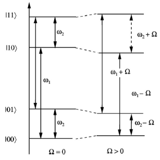
Figure 2.1: Energies of the basis states with coupling ($\Omega\neq 0$) and without coupling ($\Omega=0$). Without coupling, the signal is highly peaked around frequencies $\omega_{1}$ and $\omega_{2}$. When the coupling between spins of the corresponding NMR molecule is on, there appear four peaks due to splitting ($\omega_{1}\pm\Omega$ and $\omega_{2}\pm\Omega$). With $\omega_{2}<\omega_{1}$, this states represent the abstract computational ones $|00\rangle$, $|01\rangle$, $|10\rangle$ and $|11\rangle$.

The NMR quantum computers have poor scaling with the number of qubits. The measured signal is of the order $\alpha\,N/2^{N}$, with $\alpha=\hbar\omega/k_{B}T$ and $N$ being the number of molecules. This feature limits NMR quantum computing to applications requiring only 10 to 20 qubits [93]. Certainly, NMR technology does not offer a solution to the requirements of quantum computation. However, this technology has demonstrated the basic effects of quantum computing and quantum information.

Finally, the fact that we deal with mixed states which are weakly entangled (expansion of $\rho_{eq.}(T)$ around the maximally mixed state $\frac{1}{N}\hat{I}$) raised an interesting discussion to what extent entanglement is necessary for quantum computing [94, 95]. Even though there is still no general answer, it was shown [94] that Shor’s algorithm requires entanglement. This is indeed the case for Grover’s (see Chapter 13).

2.5.2 The ion-trap quantum computer

In the ion-trap quantum computer [73, 81] a one-dimensional lattice of identical ions is stored and laser cooled in a linear Paul trap, which is a radio frequency quadrupole trap. This linear array of ions acts as a quantum register. The trap potential strongly confines the ions radially about the trap axis, and an electrostatic potential causes the ions to oscillate along the trap axis in an effective harmonic potential (see Fig.2.2). A set of lasers shines the atoms, which are cooled so that they are localized along the trap axis, with spacing determined by Coulomb repulsion and the confining axial potential. The lowest collective excitation is the axial centre-of-mass mode (see Fig.2.2). Each of the trapped ions acts as a qubit, in which the two pertinent states are the electronic ground state and a long-lived excited state. By means of coherent interaction of a precisely controlled laser pulse with any one of the ions in a standing wave configuration, one can manipulate the ion’s electronic state and the quantum state of the collective centre of mass mode of the oscillator. The centre of mass mode can then be used as a bus, quantum dynamically connecting the qubits, to implement the necessary quantum logic gates. The general state of the line of ions comprising the quantum register is an entangled linear superposition of their states. Experimental demonstration of the ion-trap approach began with state preparation, quantum gates, and measurement for a single trapped ion [96]. Since then, a number of experimental and theoretical issues regarding the ion-trap approach to quantum computation have been explored [34].

The primary source of decoherence is apparently the heating due to coupling between the ions and noise voltages in the trap electrodes. Besides decoherence, the main goal of ion-trap set ups is to maintain an equilibrium with loading more and more ions in the trap. Also, the speed of an ion trap quantum computer would apparently be limited by the frequencies of vibrational modes in the trap.

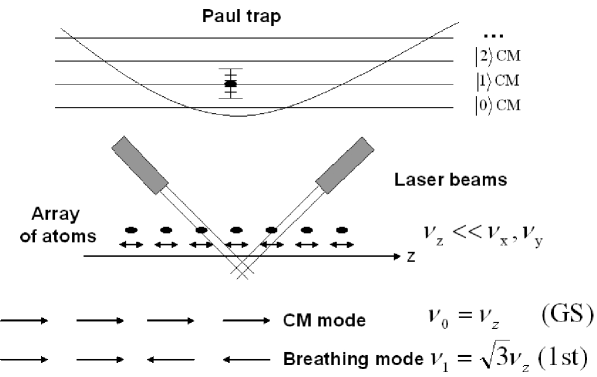
Figure 2.2: The ion-trap quantum computer confines an array of atoms along the axis of a combined electrostatic and radio frequency trap (the Paul trap). Qubits are stored in the spin states of the atoms, which can be addressed individually with high-precision lasers. The combination of internal degrees of freedom of the atom plus the quantized harmonic motion of the whole system of atoms is the basis of performing one an two-qubit gates.

2.5.3 Quantum computing using optical lattices

There exists a wide interest in the study of cold atoms confined in optical lattices, which are systems with remarkable features for quantum computing. An optical lattice [97] is essentially an artificial crystal of light, which is obtained when a periodic intensity pattern is formed by the interference of two or more laser beams. Typically, a periodic 2D intensity pattern is formed where two perpendicular standing waves interfere. The atoms sit in a regular array at every position of maximum brightness, like eggs in an egg-box. An optical lattice is able to trap atoms because the electric fields of the lasers induce an electric dipole moment in the atom [97]. If the laser frequency is less than a specific electronic transition one within the atom, they are then pulled towards regions of maximum intensity. Conversely, if the laser frequency is higher, the atoms are pushed away. These lattices are “loaded” with cold bosonic atoms which are transferred from a Bose condensate from a magnetic trap to an optical lattice. By controlling the confining lasers it is possible to move the atoms over precise separations, and even to make them contact with neighbouring atoms, with exquisite degree of control. The interesting thing about this set-up is that it is possible to convert a weakly interacting Bose gas into a Mott insulator –a strongly interacting quantum state. This proposal has been achieved experimentally [97]. When the system is in the form of a Mott insulator, each lattice is occupied by a single atom or qubit, the interaction energy is zero and there is no phase coherence between atoms. This fact converts this set-up in a perfect quantum “simulator” for several models of current study in mesoscopic systems (Hubbard model, Anderson model, etc.).

In these systems, a large number of atoms can be trapped in the lattice at very low temperatures, providing a large number of qubits. Besides, neutral atoms interact weakly with the environment, which boils down to slow decoherence times. In an experiment reported in 2004, Bloch and co-workers created a Bose Einstein condensate of Rubidium atoms, and about 10,000 them were transferred to an optical lattice. Optical lattices pose important experimental challenges, such as loading the lattice with one atom per site or being able to measure the interaction and tunnelling constants with high accuracy. See Ref. [98] for current proposals for quantum computations with neutral atoms. Very briefly, one considers a set of bosonic atoms confined in a periodic lattice at sufficiently low temperatures such that the only first Bloch band is occupied. The qubit is then stored in the two relevant ground levels $|0\rangle$ and $|1\rangle$ [98]. In [98], single qubit gates are realized using lasers and two-qubit gates are obtained by displacing the atoms in a particular internal state to a next neighbour site.

Chapter 3 Novel (or improved) aspects in quantum information: quantum communication

Entangled states have offered a new perspective on secret communication between parties, usually two parties, named Alice (A) and Bob (B). This Chapter is far from being a comprehensive study of the quantum communication features. Our aim is to grap some of the applications that are of current research interest in quantum communication. For instance, quantum channels are not discussed, though their study constitutes a basic means for successful communication. The reader is intended to Refs. [34, 87] for a comprehensive review of the subject.

3.1 Quantum dense coding

Entangled states permit a completely new way of encoding information, as first suggested by Bennett and Wiesner in 1992 [99]. Suppose Alice wants to send two bits of classical information to Bob. One possibility is to send him two particles with information encoded in their polarization states. From the point of view of (classical) information theory, two bits is the maximum Alice can send in this way. One method of doing this would be to send one of the four Bell states $|\Phi^{+}\rangle$, $|\Phi^{-}\rangle$, $|\Psi^{+}\rangle$, $|\Psi^{-}\rangle$, with probability 1/4. Suppose on the contrary that Alice and Bob share the Bell state $|\Phi^{+}\rangle$, from a EPR source. The local actions that alice can perform (on the polarization state of the entangled photons) are given by the transformations $U_{0}=\hat{I}\otimes\hat{I}$, $U_{1}=\hat{\sigma}_{x}\otimes\hat{I}$, $U_{2}=\hat{\sigma}_{y}\otimes\hat{I}$ and $U_{3}=\hat{\sigma}_{z}\otimes\hat{I}$. Applying the aforementioned transformations to $|\Phi^{+}\rangle$, we have $U_{0}|\Phi^{+}\rangle=|\Phi^{+}\rangle$, $U_{1}|\Phi^{+}\rangle=|\Psi^{+}\rangle$, $U_{2}|\Phi^{+}\rangle=-i|\Psi^{-}\rangle$ and $U_{3}|\Phi^{+}\rangle=|\Phi^{-}\rangle$.

Now Alice and Bob take out their EPR pairs, and Alice performs one of these operations on her side. She sends her qubit $A$ of pair $|\Phi^{+}\rangle$ to Bob, who performs the measurements $\sigma_{x}^{A}\sigma_{x}^{B}$ and $\sigma_{z}^{A}\sigma_{z}^{B}$ (the superindex labels the side where the particle forming the shared entangled state of two qubits $|\Phi^{+}\rangle$ comes from). Because all Bell states are eigenstates of these operators, with different eigenvalues, these measurements completely identify the state. Once Bob obtains his outcome, he can infer which of the four local operations Alice used. He has received two bits of information despite the fact that Alice only sent him one qubit (a two-level system). This is the basis of superdense coding. Quantum dense coding has been achieved experimentally by Mattle et al. from the group of Innsbruck [100], among other laboratories. The experiment relies on the process of spontaneous parametric down-conversion in a non-linear crystal, which produces pairs of photons with entangled polarizations. Quantum dense coding was the first experimental demonstration of the basics of quantum communication.

The maximum “compression factor”, so to speak, for superdense coding in the case of pure states was given by Hausladen et al. in [101], where for any pure $N$-state entangled state that Alice can send, she communicates log$N$ bits of information. As one should expect, the excess from superdense coding is exactly equal to the entanglement of the state.

3.2 Quantum teleportation

An even more interesting process in quantum communication is given by quantum teleportation. Let us suppose that Alice has an object and wants Bob the have the same object she has. In principle she could (classically) sent all information relative to that object to Bob, in order to reconstitute it. But this is forbidden in quantum mechanics, which prohibits a complete knowledge of the state of any object.

Luckily, there exists another strategy. All one has to do is to guarentee that what Bob receives has the same properties as Alice’s original, without knowing the properties of the original object, that is, without measurement. This was the Bennett’s way to avoid the measuring process through teleportation [102]. Let us suppose as in the case of dense coding that that Alice and Bob share the Bell state $|\Phi_{AB}^{+}\rangle$. Also, on one side, Alice holds an (unknown) qubit state $|\Psi\rangle_{C}=a|0\rangle_{C}+b|1\rangle_{C}$ on system $C$. Coefficients $a$ and $b$ need not be known, otherwise the teleportation scheme is not valid (a measurement process would destroy the quantum information). The nice feature about system $A\oplus B\oplus C$ is that the state $|\Phi_{AB}^{+}\rangle|\Psi\rangle_{C}$ can be written as

$$\frac{1}{2\sqrt{2}}\,\bigg{(}|\Phi^{+}\rangle_{AC}(a|0\rangle_{B}+b|1\rangle_{B})+|\Phi^{-}\rangle_{AC}(a|0\rangle_{B}-b|1\rangle_{B})+$$ (3.1)

$$|\Psi^{+}\rangle_{AC}(a|0\rangle_{B}+b|1\rangle_{B})+|\Psi^{-}\rangle_{AC}(a|0\rangle_{B}-b|1\rangle_{B})\bigg{)}.$$ (3.2)

Alice then performs a joint Bell-state measurement on the photon se wants to teleport and one of the ancilliary photons. This measurement projects the other ancillary photon into a quantum state (one of the four in (3.1)), which is uniquely linked to $|\Psi\rangle$ up to some rotations. Alice then telephones Bob, telling him the result of her measurement. All Bob has to do is to perform the appropriate operation on his qubit and ends up with the state $|\Psi\rangle$.

No faster than speed of light transmission of information takes place, as one might wonder. Quantum teleportation does not violate causality because it requires a means of classical communication in order to restore the original state. Quantum teleportation has been experimentally realized using single photons [103, 104] and nuclear spins as qubits (NMR techniques) [105]. Recently, the group of R. Blatt reported the teleportation of the quantum state of a trapped calcium ion to another calcium ion [106], and the group of M. D. Barrett reported a similar experiment with beryllium ions [107]. Ref. [108] offers a critical view of the nuts and bolts of the experimental and theoretical status of teleportation. Still, we are far from Star Trek.

3.3 Quantum cryptography

“Shaken, not stirred.”

Bond, James Bond.

Quantum cryptography, also known as quantum key distribution (QKD), exploits the principles of quantum mechanics to enable secure distribution of private communication. The scenario is the following: we have Alice and Bob who want to communicate with each other, and an eavesdropper Eve, who wants to “listen” to what they say. In classical cryptography, public key distribution is widely used in the Internet in the form of the RSA cryptosystem, developed by Rivest, Shamir, and Adleman in 1978 [109]. Its security lies on the difficulty of factorizing large numbers with the available classical algorithms, even for supercomputers. It is based on secret key sharing and public key distribution. Suppose that Alice has her the message $Y$ encoded in a string of bits (an integer number), and so does Bob with $Z$, both of them being private and random. $X$ and $N$ are public and random. Alice perfoms $X^{Y}$mod$N$ on her side, while Bob does the same thing with $X^{Z}$mod$N$. Now they exchange information. Alice will have $(X^{Z}{\rm mod}N)^{Y}$mod$N$=$(X^{ZY}{\rm mod}N)$ and Bob $(X^{Y}{\rm mod}N)^{Z}$mod$N$=$(X^{YZ}{\rm mod}N)$, which is clearly the same message. These operations are easy to do. For Eve to find the secret message $(X^{ZY}{\rm mod}N)$, knowing $X$, $N$, $X^{Y}$mod$N$ and $X^{Z}$mod$N$ (all public stuff), would require a very long time with a classical algorithm.

A quantum computer would factorize numbers quickly in the RSA scenario, thus revealing secret messages. This is why, among other reasons, quantum cryptography is the most mature area of quantum information, both at the theoretical and experimental level (it has been demonstrated over distances of tens of kilometres!). See Ref. [110] for a comprehensive survey of experimental results. However, this does not imply that a classical breaking of the RSA cryptosystem is not possible. A classical algorithm –in case of existence– that factorizes large integers in a polynomial number of steps, has not yet been found.

In the context of QKD, using the quantum mechanical properties of information carriers, Alice and Bob can generate a truly random sequence of classical bits - 0’s and 1’s - which they both know perfectly, unknown by any third party. If Alice and Bob share a secret key in this way, they can transmit information completely securely over a public (insecure) channel. They do this by using the One-Time Pad, which is the only guaranteed unbreakable code known. If Alice wishes to send the secret message 101110 to Bob and they share a secret key 001011, then by bitwise-adding the message and the key she arrives at the encrypted message 100101 which she sends to Bob. By bitwise-adding the secret key to the message, Bob uncovers the original message. It can be shown that, as long as Alice and Bob use the secret key only once, an eavesdropper Eve can obtain no information about the message [34]. The problem is how to share a secret key with someone when one cannot decide on a capable courier to carry it. There are several protocols in QKD that solve this problem using properties of quantum mechanics. The first one is the BB84 protocol, conceived by Bennett and Brassard in 1984 [111]. Let us encode the information in the polarization state of a photon. First Alice chooses randomly one state out of four (four non-orthogonal vectors in $C^{2}$), and sends a qubit to Bob. Then, Bob measures the qubits that receives (he selects two operators, say $\hat{\sigma}_{x},\hat{\sigma}_{z}$) and obtain the outcomes. After this there is a public discussion (classical communication), where they want to get rid of the uncorrelated results (both look at the coincidences and erase those which are uncorrelated). Finally there comes an authentification, where they check that nobody has been listening. They can do so because due to the quantum measurement Eve disturbs the system when she tries to obtain information. Also, as we shall see, she cannot make perfect copies of states by virtue of the non-cloning theorem. Therefore secret communication is based on basic principles of quantum mechanics.

3.4 The non-cloning theorem and quantum repeaters

Perfect copies of classical bits of information are carried out in everyday life technology. The copy-paste routine of text editors is possible because classical information can be copied at will. It took considerable long time to realize that this simple procedure is not possible in the quantum domain. This is the surprising “Non-cloning Theorem” due to W. K. Wootters and W. H. Zurek [112]. Let us consider the Hilbert space $H_{n}$ of a system having $n$ basis states $\{|a_{1}\rangle...|a_{n}\rangle\}$. The action of cloning a given state $|a_{1}\rangle$ is given by a unitary mapping in $H_{n}\otimes H_{n}$ that, for any state $|{\bf x}\rangle\in H_{n}$, results in $U(|{\bf x}\rangle|a_{1}\rangle)=|{\bf x}\rangle|{\bf x}\rangle$. The proof that this is not possible is so simple that it can be done in few lines. Assume that a quantum copymachine exists and $n>1$. Therefore two orthogonal states $|a_{1}\rangle$ and $|a_{2}\rangle$ exist. The application of the copymachine leads to $U(|a_{1}\rangle|a_{1}\rangle)=|a_{1}\rangle|a_{1}\rangle$ and $U(|a_{2}\rangle|a_{1}\rangle)=|a_{2}\rangle|a_{2}\rangle$. Combining both of them, we have

$$U\big{(}\frac{1}{\sqrt{2}}(|a_{1}\rangle+|a_{2}\rangle)\,|a_{1}\rangle\big{)}\, = \,\big{(}\frac{1}{\sqrt{2}}(|a_{1}\rangle+|a_{2}\rangle)\,\frac{1}{\sqrt{2}}(|a_{1}\rangle+|a_{2}\rangle)\big{)}$$ (3.3)

$$= \,\frac{1}{2}\,(|a_{1}\rangle|a_{1}\rangle+|a_{1}\rangle|a_{2}\rangle+|a_{2}\rangle|a_{1}\rangle+|a_{2}\rangle|a_{2}\rangle).$$ (3.4)

Owing to linearity of $U$, we also have

$$U\big{(}\frac{1}{\sqrt{2}}(|a_{1}\rangle+|a_{2}\rangle)\,|a_{1}\rangle\big{)}\, = \,\frac{1}{\sqrt{2}}U(|a_{1}\rangle|a_{1}\rangle)\,+\,\frac{1}{\sqrt{2}}U(|a_{2}\rangle|a_{1}\rangle)$$ (3.5)

$$= \,\frac{1}{\sqrt{2}}\,(|a_{1}\rangle|a_{1}\rangle)\,+\,\frac{1}{\sqrt{2}}\,(|a_{2}\rangle|a_{2}\rangle).$$ (3.6)

Formulas (3.3) and (3.5) clearly do not coincide. We thus have arrived to a contradiction and a quantum state cannot be perfectly cloned.

We just have shown that a quantum state cannot be perfectly cloned, but this fact does not mean that imperfect copies of states can be supplied, with a degree of accuracy (as measured by so called fidelity $F$) high enough so that certain processes of quantum communication are possible.

The non-cloning theorem has to be taken into account in the design of quantum channels. Because of decoherence and absorption by fibres, entangled pair of particles (or qubits, photons in this case) can only be maintained through finite lenghts, so it is required a number of repetitions, hence quantum repeaters, for a succesful transmission. Amplification of the qubit cannot be done without destroying the quantum correlations present [112]. A solution [87] is obtained in a way simmilar to classical communication. The channel is divided in $N$ parts, where a combination of fidelity-enhancement, entanglement purification and entanglement swapping take place in small “quantum processors” (composed by a few qubits) at every connection point. See Ref. [87] and [113] for more details on quantum repeaters.

Part II Quantum Entanglement

Chapter 4 Detection of entanglement

Entanglement is one of the most fundamental and non-classical features exhibited by quantum systems [110], that lies at the basis of some of the most important processes studied by quantum information theory [12, 34, 110, 114, 115] such as quantum cryptographic key distribution [116], quantum teleportation [102], superdense coding [99], and quantum computation [72, 117]. It is plain from the fact that entanglement is an essential feature for quantum computation or secure quantum communication, that one has to be able to develop some procedures (physical or purely mathematical in origin) so as to ascertain whether the state $\rho$ representing the physical system under consideration is appropriate for developing a given non-classical task. Besides, detecting entanglement is a way of characterizing the system possessing quantum correlations, a fundamental physical property that need not have to find any application whatsoever.

In this chapter we state the so called “separability problem”, which is of great importance in quantum information theory, and expose the methods or criteria (operational and non-operational) available in order to detect quantum entanglement. Unless explicitly stated we consider entanglement between two parties, which is the common situation, say, in quantum communication protocols. Although some results can be extended to multipartite systems easily, some other scenarios are either under current research or remain open questions, in the same manner that some problems in the bipartite case have not yet been solved.

4.1 The separability problem

As pointed out before, it is essential to discriminate the states that contain classical correlations only. Historically, the violation of Bell’s inequalities have become equivalent to non-locality or, in our this context, to entanglement. For every pure entangled state there is a Bell inequality that is violated and, in consequence, from a historic viewpoint, the first separability criterion is that of Bell (see [118] and references therein). It is not known, however, whether in the case of many entangled mixed states, violations exist: some states, after “distillation” of entanglement (this is done by performing local operations and classical operations (LOCC), that is, operations performed on each side independently) eventually violate the inequalities, but some others don’t.

The first to point out that an entangled state did not imply violation of Bell-type inequalities (that is, they admit a local hidden variable model) was Werner [42], providing himself with a family of mixed states (the Werner $\rho_{W}$) that do no violate the aforementioned inequalities. Werner also provided the current mathematical definition for separable states: a state of a composite quantum system constituted by the two subsystems $A$ and $B$ is called “entangled” if it can not be represented as a convex linear combination of product states. In other words, the density matrix $\rho_{AB}\in{\cal H}_{A}\otimes{\cal H}_{B}$ represents an entangled state if it cannot be expressed as

$$\rho_{AB}\,=\,\sum_{k}\,p_{k}\,\rho_{A}^{(k)}\otimes\rho_{B}^{(k)},$$ (4.1)

with $0\leq p_{k}\leq 1$ and $\sum_{k}p_{k}=1$. On the contrary, states of the form (4.1) are called separable. The above definition is physically meaningful because entangled states (unlike separable states) cannot be prepared locally by acting on each subsystem individually [119] (LOCC operations). An example of a LOCC operation is provided by

$$\rho\prime\,=\,(U_{A}\otimes U_{B})\,\rho\,(U_{A}\otimes U_{B})^{\dagger},$$ (4.2)

where $U_{A}$($U_{B}$) represents a local action (unitary transformation) acting on subsystem $A$($B$). Equivalently, a separable state is a state that can be written as a mixture of factorizable pure states. Apparently this should be the end of the story. If one is able to write a given state as a convex combination of product states as in (4.1), then that state is separable. In practice, though, this is an impossible task because there are infinitely many ways of decomposing a state $\rho$ (for instance, the pure states constituting the alluded mixture need not be orthogonal, what makes it even more arduous). Physically, it means that the state can be prepared in many ways. Another intriguing feature is that a mixture of entangled states is not necessary entangled. On the contrary, the set of separable or unentangled states is convex: any linear convex combination of separable states gives another separable state. Thus we arrive at the separability problem: given a state $\rho$ describing a quantum system, is it entangled or not?

This (not generally solved) problem can be related, as we shall see, to challenging open questions of modern linear algebra: the characterization of positive maps. However, we require a criterion which could decide wheter a state $\rho$ is entangled or not. Such procedure can be cast following a simple algorithm or recipe (a functional criterion) or abstractly (a non-functional criterion). The next sections give an account of such criterions.

4.2 Functional criteria: PPT, reduction, majorization and $q$-entropic. Inclusion relations among them

The development of criteria for entanglement and separability is one aspect of the current research efforts in quantum information theory that is receiving, and certainly deserves, considerable attention [118]. Indeed, much progress has recently been made in consolidating such a cornerstone of the theory of quantum entanglement [118]. Before discussing the general mixed case, we must mention that there is a simple necessary and sufficient separability criterion for pure states, namely, the Schmidt decomposition [118]. Given a pure state $\rho_{AB}\in{\cal H}_{A}\otimes{\cal H}_{B}$, $N$ being the dimension of system $A$ and $M\geq N$ the one for system $B$, with rank $r\leq N$, it can be decomposed as a sum of products of orthogonal states

$$|\Psi\rangle\,=\,\sum_{i=1}^{r}w_{i}|x_{i}\rangle\otimes|y_{i}\rangle,$$ (4.3)

with $w_{i}>0$ and $\sum_{i=1}^{r}w^{2}_{i}=1$, $\langle x_{i}|x_{j}\rangle=\langle y_{i}|y_{j}\rangle=\delta_{ij}$. The criterion is then extremely simple: a the state $|\Psi\rangle$ is separable or unentangled iff $r=1$.

Returning to the mixed case, from the formal point of view it was shown by the Horodecki family (see [118] and references therein) that a density matrix $\rho\equiv\rho_{AB}$ is entangled if and only if there exists an entanglement witness (a hermitian operator $\hat{W}=\hat{W}^{\dagger}$) such that

$$Tr\,\hat{W}\,\hat{\rho} \leq 0,\,\,\,\,{\rm while}$$

$$Tr\,\hat{W}\,\hat{\rho}_{s} \geq 0,\,\,{\rm for\,\,all\,\,separable\,\,states\,\,\rho_{s}}.$$ (4.4)

This rather abstract definition (it defines what is called an entanglement witness) exposes the need of more operational criteria that are easy to check in an explicit case. Let us briefly sketch the situation of the state-of-the-art functional criteria, and later on explain in more detail each one of them. A special, but quite important LOCC operational separability criterion, necessary but not sufficient, is provided by the positive partial transpose (PPT) one. Let $T$ stand for matrix transposition. The PPT requires that

$$[\hat{1}\otimes\hat{T}](\rho)\geq 0.$$ (4.5)

Another operational criterion is called the reduction criterion, that is satisfied, for a given state $\rho\equiv\rho_{AB}$, when both [118]

$${\hbox{\Bbb I}}\otimes\rho_{B}-\rho \geq 0$$

$$\rho_{A}\otimes{\hbox{\Bbb I}}-\rho \geq 0.$$ (4.6)

Intuitively, the distillable entanglement is the maximum asymptotic yield of singleton states that can be obtained, via LOCC, from a given mixed state. Horodecki et al. [120] demonstrated that any entangled mixed state of two qubits can be distilled to obtain the singleton. This is not true in general. There are entangled mixed states of two qutrits, for instance, that cannot be distilled, so that they are useless for quantum communication. These are the so called bound entangled states. An important fact is that all states that violate the reduction criterion are distillable [121].

Another criterion associates PPT to the rank of a matrix. Consider two subsystems $A$, $B$ whose description is made, respectively, in the Hilbert spaces ${\cal H}_{n}$ and ${\cal H}_{m}$. Focus attention now in the density matrix $\rho\equiv\rho_{AB}$ for the associated composite system. If

1. $\rho$ has PPT, and

2. its rank ${\cal R}$ is such that ${\cal R}\leq{\rm max}(n,m)$,

then, as was proved in [122], $\rho$ is separable.

The entropic criteria are also functional separability ones. Still another one is majorization.

PPT

The PPT criterion was suggested by Peres in [123]. So far, it has been shown to be the strongest criterion providing the closest approximation to the set of separable states. Formally, it can be cast in the following way. Let $\rho_{AB}$ be a generic state of a bipartite Hilbert space ${\cal H}={\cal H}_{A}\otimes{\cal H}_{B}$, with $N_{A}$ and $N_{B}$ the dimensions of the concomitant subsystems. If we express $\rho\equiv\rho_{AB}$ in the corresponding ortonormal product basis

$$\rho\,=\,\sum_{i,j=1}^{N_{A}}\sum_{m,n}^{N_{B}}\langle i,m|\rho|,j,n\rangle\,|i,m\rangle\langle j,n|\,=\,\sum_{i,j=1}^{N_{A}}\sum_{m,n}^{N_{B}}\langle i,m|\rho|,j,n\rangle\,|i\rangle_{A}\langle j|\otimes|m\rangle_{B}\langle n|,$$ (4.7)

the partial transpose with respect to $A$ is given by

$$\rho^{T_{A}}\,=\,\sum_{i,j=1}^{N_{A}}\sum_{m,n}^{N_{B}}\langle i,m|\rho|,j,n\rangle\,|{\bf j}\rangle_{A}\langle{\bf i}|\otimes|m\rangle_{B}\langle n|.$$ (4.8)

If $\rho$ is separable, then $\rho^{T_{A}}$ must have all their eigenvalues defined positive (positive operator). The reverse it was conjectured to be true. In Fig.4.1 we provide a pictorial image of partial trasposition in system of two qubits, expressed in the so called computational basis ($|0_{A}\rangle\otimes|0_{B}\rangle,|0_{A}\rangle\otimes|1_{B}\rangle,|1_{A}\rangle\otimes|0_{B}\rangle,|1_{A}\rangle\otimes|1_{B}\rangle$). A state that fullfils $\rho^{T_{A}}\geq 0$ is called PPT, otherwise NPT. If a state $\rho$ is separable, that is, it can be written as (4.1), then it must possess a $\rho^{T_{A}}\geq 0$. It was shown by the Horodecki family [124] with use of positive maps, that PPT in systems of dimensions $2\times 2$ and $2\times 3$ is not only necessary but sufficient for separability.

Figure 4.1: Pictorial action of partially transposing a state $\rho$ in the computational basis $|00\rangle,|01\rangle,|10\rangle,|11\rangle$. PPT action on subsystem $A$ moves the matrix elements as shown is the figure.

The physical significance of the positivity of (4.8) is the following. Precisely, it’s all about producing unphysical results. Taking the partial transposition of a separable state $\rho$, which can be written in the form (4.1), does not produce any new matrix due to the fact that (4.1) factorizes, and therefore must be a valid state (must remain positive). If applied to a state that is entangled, then it can give an unphysical result (some negative eigenvalue). Partial transposition is equivalent to time reversal on either one of the parties!

Reduction

The reduction criterion certainly resembles PPT in the fact that a certain operation is done on one of the subsystems independently. What lies beneath is more about positive maps, and will be apparent from the discussion in the next section. Quite recently [125] it was shown that if a bipartite quantum state satisfies the reduction criterion for distillability, then it satisfies the majorization criterion for separability, therefore stablishing a strong link between reduction and the next criterion.

Majorization

Let $\{\lambda_{i}\}$ be the set of eigenvalues of the matrix $\xi_{1}$ and $\{\gamma_{i}\}$ be the set of eigenvalues of the matrix $\xi_{2}$. We assert that the ordered set of eigenvalues $\vec{\lambda}$ of $\xi_{1}$ majorizes the ordered set of eigenvalues $\vec{\gamma}$ of $\xi_{2}$ (and writes $\vec{\lambda}\succ\vec{\gamma}$) when $\sum_{i=1}^{k}\,\lambda_{i}\,\geq\,\sum_{i=1}^{k}\,\gamma_{i}$ for all $k$. It has been shown [126] that, for all separable states $\rho_{AB}\equiv\rho$,

$$\vec{\lambda}_{\rho_{A}} \succ \vec{\lambda}_{\rho},\,\,{\rm and}$$

$$\vec{\lambda}_{\rho_{B}} \succ \vec{\lambda}_{\rho}.$$ (4.9)

This last fact can be cast in the following sentence: separable states are more disordered globally than locally.

In point of fact, it is not possible to find a necessary and sufficient criterion for separability based solely upon the eigenvalue spectra of the three density matrices $\rho_{AB},\rho_{A}=Tr_{B}[\rho_{AB}]$, and $\rho_{B}=Tr_{A}[\rho_{AB}]$ associated with a composite system $A\oplus B$ [126]. That is why both majorization and the $q$-entropic criterions are weaker than PPT. Besides, there is an intimate relation between this majorization criterion and entropic inequalities, as discussed in [118, 127]: if a state is separable in view of the reduction criterion then it must comply with the $q$-entropic criterion.

$q$-Entropic

The separability question has quite interesting echoes in information theory and its associate information measures or entropies. When one deals with a classical composite system described by a suitable probability distribution defined over the concomitant phase space, the entropy of any of its subsystems is always equal or smaller than the entropy characterizing the whole system. This is also the case for separable states of a composite quantum system [126, 127]. In contrast, a subsystem of a quantum system described by an entangled state may have an entropy greater than the entropy of the whole system. Indeed, the von Neumann entropy of either of the subsystems of a bipartite quantum system described (as a whole) by a pure state provides a natural measure of the amount of entanglement of such state. Thus, a pure state (which has vanishing entropy) is entangled if and only if its subsystems have an entropy larger than the one associated with the system as a whole.

Regrettably enough, the situation is more complex when the composite system is described by a mixed state. There are entangled mixed states such that the entropy of the complete system is smaller than the entropy of one of its subsystems. Alas, entangled mixed states such that the entropy of the system as a whole is larger than the entropy of either of its subsystems do exist as well. Consequently, the classical inequalities relating the entropy of the whole system with the entropy of its subsystems provide only necessary, but not sufficient, conditions for quantum separability. There are several entropic (or information) measures that can be used in order to implement these criteria for separability. Considerable attention has been paid, in this regard, to the $q$-entropies [118, 127, 128, 129, 130, 131, 132, 133, 134], which incorporate both Rényi’s [135] and Tsallis’ [136, 137, 138] families of information measures as special instances (both admitting, in turn, Shannon’s measure as the particular case associated with the limit $q\rightarrow 1$). Here we recall the definitions that appear in the Introduction.

The “$q$-entropies” depend upon the eigenvalues $p_{i}$ of the density matrix $\rho$ of a quantum system through the quantity $\omega_{q}=\sum_{i}p_{i}^{q}$. More explicitly, we shall consider either the Rényi entropies [135],

$$S^{(R)}_{q}\,=\,\frac{1}{1-q}\,\ln\left(\omega_{q}\right),$$ (4.10)

or the Tsallis’ entropies [136, 137, 138]

$$S^{(T)}_{q}\,=\,\frac{1}{q-1}\bigl{(}1-\omega_{q}\bigr{)},$$ (4.11)

which have found many applications in many different fields of Physics. These entropic measures incorporate the important (because of its relationship with the standard thermodynamic entropy) instance of the von Neumann measure, as a particular limit ($q\rightarrow 1$) situation

$$S_{1}\,=\,-\,Tr\left(\hat{\rho}\ln\hat{\rho}\right).$$ (4.12)

The concomitant ${\it conditional\,q-entropies}$ are defined as

$$S^{(T)}_{q}(A|B)\,=\,\frac{S^{(T)}_{q}(\rho_{AB})-S^{(T)}_{q}(\rho_{B})}{1+(1-q)S^{(T)}_{q}(\rho_{B})}$$ (4.13)

for the Tsallis case, while its Rényi counterpart is

$$S^{(R)}_{q}(A|B)\,=\,S^{(R)}_{q}(\rho_{AB})-S^{(R)}_{q}(\rho_{B}),$$ (4.14)

where $\rho_{B}=Tr_{A}(\rho_{AB})$ (the conditional $q$-entropy $S^{(T)}_{q}(B|A)$ is defined in a similar way as (4.13), replacing $\rho_{B}$ by $\rho_{A}=Tr_{B}(\rho_{AB})$). The “classical $q$-entropic inequalities” finally read

$$S^{(T,R)}_{q}(A|B) \geq 0,$$ (4.15)

$$S^{(T,R)}_{q}(B|A) \geq 0,$$ (4.16)

accomplished by all separable states for several $q$-values [121].

The early motivation for the studies reported in [127, 128, 129, 130, 131, 132, 133, 134] was the development of practical separability criteria for density matrices. The discovery by Peres of the partial transpose criteria, which for two-qubits and qubit-qutrit systems turned out to be both necessary and sufficient, rendered that original motivation somewhat outmoded. However, their study provide a more physical insight into the issue of quantum separability.

We have shown that all these criterions obey a chain of implications: if a state complies with PPT, it follows that it must satisfy reduction; in turn, majorization is satisfied, as well as the entropic inequalities [139]. Symbolically, we have

${\it\rho\,\,separable\rightarrow PPT\rightarrow reduction\rightarrow majorization\rightarrow q-entropic}$.

None of the implication relations can be reversed for a general state, except for systems in $2\times N_{B}$ dimensions, where reduction is equivalent to PPT. Also, PPT provides a necessary and sufficient condition in $2\times 2$ and $2\times 3$ dimensions. This implications and other results are exhaustively studied in Chapter 7.

4.3 Non-functional criteria: the theory of positive maps and entanglement witnesses

The criterions described in this section are not easy to implement in practice, but nevertheless constitute necessary and sufficient means of discriminated whether a state $\rho$ possesses entanglement or not.

There is an interesting connection between entanglement and the theory of positive maps [140], which requires some mathematical definitions regarding positive operators, positive and completely positive maps. First of all we recall that any physical action is represented by a positive map. Let us suppose that ${\cal O}_{A}$ and ${\cal O}_{B}$ denote the set of operators acting on the subsystems of ${\cal H}={\cal H}_{A}\otimes{\cal H}_{B}$, and let us denote by $L({\cal O}_{A},{\cal O}_{B})$ the space of the linear maps from ${\cal O}_{A}$ to ${\cal O}_{B}$. Then, a map $\Lambda\in L({\cal O}_{A},{\cal O}_{B})$ is said to be positive if it maps positive operators in ${\cal O}_{A}$ into positive operators.

Completely positive is an extension of the previous maps. A map $\Lambda\in L({\cal O}_{A},{\cal O}_{B})$ is completely positive if the extended map

$$\Lambda_{x}=\Lambda\otimes{\hbox{\Bbb I}}_{x}:{\cal O}_{A}\otimes{\cal M}_{x}\rightarrow{\cal O}_{B}\otimes{\cal M}_{x}$$ (4.17)

is positive for all extensions of dimension $x$, where ${\hbox{\Bbb I}}_{x}$ is the identity map on the space ${\cal M}_{x}$. Now here we have the desired characterisation of separable states via positive maps, bearing in mind that complete positivity is not equivalent to positivity. A state is separable iff for any positive map [140] $\Lambda$

$$({\hbox{\Bbb I}}\otimes\Lambda)\rho\geq 0$$ (4.18)

holds.

Interpretation of PPT is thus straightforward if we regard the action of partial transposition in (4.8) as an extension on the total transposition $\hat{T}$ of a state (a positive map that leaves the positive eigenvalues of $\rho$ untouched): $[{\hbox{\Bbb I}}\otimes\hat{T}](\rho)\geq 0$ (or its dual form $[\hat{T}\otimes{\hbox{\Bbb I}}](\rho)\geq 0$). Thus, a state $\rho$ that verifies PPT (thus separable) has an associated completely positive map. The fact that systems in low dimensions can be characterised without much difficulty, allow us to ascertain that PPT is a necessary and sufficient criterion for $2\times 2$ and $2\times 3$ systems ($\Lambda:M_{2}\rightarrow M_{2}$, $\Lambda:M_{3}\rightarrow M_{2}$). However, the problem remains open (here we have the link with unsolved challenges of modern mathematics) because the full description of separability is equivalent to the characterization of the set of all positive maps, which is per se a formidable task.

The reduction criterion can also be reviewed in terms of positive maps. In this case, the map under consideration is given by $\Lambda({\cal O})=$Tr$({\cal O}){\hbox{\Bbb I}}-{\cal O}$. The eigenvalues of the resulting operator $\Lambda({\cal O})$ are given by $\lambda_{i}=$Tr$({\cal O})-o_{i}$ where $o_{i}$ are eigenvalues of $O$. It follows immediately that if ${\cal O}\geq 0$, the map is positive ($\lambda_{i}\geq 0$). Taking the formula (4.18) and its dual form $(\Lambda\otimes{\hbox{\Bbb I}})\rho\geq 0$ for the aforementioned map, the following inequalities

$${\hbox{\Bbb I}}\otimes\rho_{B}-\rho\geq 0,\quad\rho_{A}\otimes{\hbox{\Bbb I}}-\rho\geq 0\,$$ (4.19)

must be observed by separable states. That is, a separable state must remain a physical operator (non-negative eigenvalues) under the action of a complete positive map. If not, there is room for entanglement.

The next non-functional criterion is the one provided by entanglement witnesses, which is, roughly speaking, a kind of Bell inequality. As already stated, $\rho$ is entangled if and only if there exists an entanglement witness (a hermitian operator $\hat{W}=\hat{W}^{\dagger}$) such that

$$Tr\,\hat{W}\,\hat{\rho} \leq 0,\,\,\,\,{\rm while}$$

$$Tr\,\hat{W}\,\hat{\rho}_{s} \geq 0,\,\,{\rm for\,\,all\,\,separable\,\,states\,\,\rho_{s}}.$$ (4.20)

As expected from linear algebra, which is the mathematical framework of these non-functional criterions, there is a correspondence between the two approaches. They are linked together through the Jamiolkowski isomorphism [141]. Here we do not expose the details of the relation between them, focusing our attention only in the properties of entanglement witnesses.

As stated, there is a fundamental difference between the set of separable or unentangled states ${\cal S}_{sep}$ and the remaining entangled states ${\cal S}-{\cal S}_{sep}$ (${\cal S}$ being the set of all states): while the former is convex, that is, any linear convex combination of separable states gives another separable state, we find counterexamples to the latter. As a consequence, the mathematical grounds for the existence of entanglement witnesses lie basically in the fact that ${\cal S}_{sep}$ is convex and compact . This allow us to introduce the Hahn-Banach theorem [142]: For any convex, compact subset ${\cal S}_{sep}$ of a finite Hilbert space ${\cal H}$ and $\rho\not\in{\cal S}_{sep}$, there exist a hyperplane $W$ that separates $\rho$ from ${\cal S}_{sep}$. Fig.4.2 illustrates this fact.

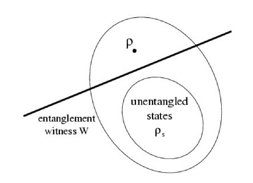
Figure 4.2: Hyperplane $W$ that separates the entangled state $\rho$ from the set of separable states ${\cal S}_{sep}$. See text for details.

Noting that Tr$(W\rho)$ is nothing but an inner product for operators in ${\cal H}$, it can be regarded as a scalar product (indeed Tr$(W)=1$) of two vectors, where the orientation of the hyperplane is taken such that separable states always lie on the positive side, whereas the entangled ones remain on the negative side (4.3). From Fig.4.3 we see that parallel transports of witness $W$ can be performed until it becomes “tangent” to ${\cal S}_{sep}$, which defines an optimal witness $W_{opt}$. By no means this is the end of the story, because one then has to perform a minimization over all possible optimal $\{$$W_{opt}$$\}$ (see Fig.4.4), which is tantamount to explore the whole shape of ${\cal S}_{sep}$ and, unless it is a polytope, it is an impossible task. Thus, the difficulty of the complete characterization of all positive maps here is translated into the complexity of “moulding” the egg-type shape of ${\cal S}_{sep}$. Nevertheless several steps have been done towards a better characterization on entanglement using these operator witnesses.

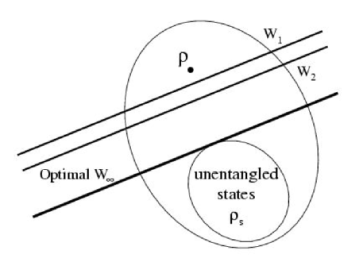
Figure 4.3: There exist different witnesses. Once a “direction” in the space of mixed states is given, the optimal witness $W_{\infty}$ is reached ($W$ “tangent” to ${\cal S}_{sep}$). See text for details.

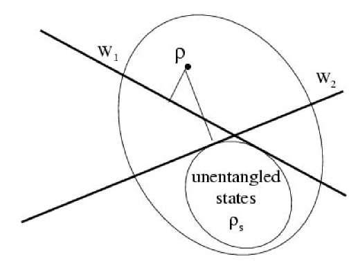
Figure 4.4: Entanglement witnesses $W_{1}$ and $W_{2}$ are optimal. The witness we seek is obtained after a survey of all optimal witnesses. See text for details.

Lots of fruitful results have been obtained with the theory of entanglement witnesses, when applied not only to separability, but also to the distillability problem. The work [143] reviews the achievements of the active group of Hannover and Innsbruck. Nevertheless, there is no general procedure for obtaining an optimal witness for a given arbitrary state $\rho$ yet.

The problem of distillability, that is, given a certain state $\rho$, the possibility of ascertaining whether it is distillable or not, follows the footsteps of the separability problem. One way of solving to problem finds its way in a non-operational criteria, which turns out to be necessary and sufficient [143]: The state $\rho$ is distillable iff there exists $|\psi\rangle=a_{1}|e_{1}\rangle|f_{1}\rangle+a_{2}|e_{2}\rangle|f_{2}\rangle$ such that $\langle\psi|(\rho^{T_{A}})^{\otimes n}|\psi\rangle<0$ for some n. The operational criteria provide some insight into the problem, but still remains open.

4.4 Schematics of the set of all states

Bipartite quantum states are classified into three categories: separable states, bound entangled states, and free entangled states. It is of great relevance to completely characterize these families of states for the full development of quantum information theory. We recall that PPT is the strongest operational criterion known to date, which provides a necessary condition for separability in any bipartite system, being indeed sufficient for cases of small dimensionality ($2\times 2$ and $2\times 3$ systems). Also, bound entangled states are those which preserve positivity (positive eigenvalues) under the action of partial transposition (PPT) and cannot be distilled. In the following, we clarify the meaning of distillation.

Thus, in view of the existence of these particular states, the set of all states ${\cal S}$ must be described either according to the separability problem (through PPT) or the distillability problem (PPT + reduction/majorization).

4.4.1 Decomposition according to PPT

If we are interested only in the separability problem, the only operational tool that we have at hand in order to describe the entanglement properties of the set ${\cal S}$ is the positive partial transposition (PPT). While waiting for a new general and more restrictive separability criterion, we discriminate states according to PPT in Fig.4.5. The only clear solution provided by PPT is restricted to low dimensions, alas, simple states easily described by positive maps or entanglement witnesses. Such states are the two-qubits systems ($2\times 2$) and the qubit-qutrit systems ($2\times 2$).

Figure 4.5: a) Decomposition of mixed states according to PPT for $2\otimes 2$ and $2\otimes 3$ systems and b) for higher dimensions (after [140]).

4.4.2 Decomposition according to distillability. Bound entanglement

It is known that the creation of maximally (ergo, pure) entangled states is possible in principle, but the most common situation encountered in practice is that those pure states evolve to mixed states due to interactions with the environment. This is the norm, for instance, whenever trying to create entangled pairs of photons for quantum communication protocols. Thus we are naturally led to the idea of distillation: we must concentrate the entanglement present in the mixed state by LOCC operations. Therefore, the classification of bipartite states according to their distillability properties is an important problem in quantum information theory.

There is something strange about those mixed states that, being already entangled, cannot be distilled: bound entangled states are invariant under the operation of partial transposition. Physically, it means that they remain physical under the unphysical action of partial transposition (time-reversal on one side only). Undistillable – separable and bound entangled – states have a common property when viewed through the glass of the characterized separability criteria: the eigenvalue vector of the global system is majorized by that of the local system. In other words, the majorization criterion is implied by reduction, and both of them constitute sufficient conditions for distillability of bipartite quantum states. Thus, whenever any of these criterions is violated, the state is distillable (the converse is not true). Using these tools, we characterize the set ${\cal S}$ of all states according to their distillability features in Fig.4.6. We must point out that that PPT and reduction coincide in $2\times N_{B}$ systems, and particularly in $2\times 2$ and $2\times 3$ systems – which are distillable (have got no bound entanglement) – PPT is also a sufficient criterion for separability.

Figure 4.6: a) Decomposition of mixed states according to distillability for $2\otimes 2$ and $2\otimes 3$ systems and b) for higher dimensions (after [140]).

Chapter 5 Characterization of entanglement

Detecting entanglement may not be sufficient. Given a matrix $\rho$ representing the state of the system, it is possible that interaction with environment destroys the entanglement present in $\rho$. We therefore require a means of quantifying entanglement. This feature, quantification, it is decisive whenever we must decide whether the entanglement provided by a physical set up (e.g. a certain physical implementation for quantum computation) is sufficient or not in order to accomplish with the quantum information related tasks. One such dramatic example is provided by nuclear magnetic resonance (NMR) computing, as explained throughout this Chapter.

A fundamental question remains still. The characterization of entanglement obviously implies a knowledge of the physical meaning of entanglement itself. In point of fact entanglement should be regarded as a resource, like energy, which underlies most of the striking new applications of the newborn science of quantum information. This extremely non-classical feature that is assumed to be the characteristic feature of quantum mechanics – even more than the superposition of possible states of a particle or the impossibility of attribution of a priori well defined properties to quantum states (problem of measurement) – looses its merely fundamental aspect in physics and finds lots of practical applications impossible to achieve before. This is perhaps what is more striking about entanglement, and indeed it is hardly possible to find a similar analogue that had undergone a similar transition in quantum mechanics.

However, we have not answered the question regarding the meaning of entanglement. As a matter of fact, no one really knows what entanglement is. This is a similar problem encountered whenever trying to define the absolute meaning of the word “energy”. In an analogous way, one describes the spectra of capacities for what entanglement is able to perform instead. This situation is somewhat similar to the historical development of Thermodynamics. The familiar entropy appeared in order to clarify the processes involving temperature, work and heat, and one had to find links to that newborn quantity through specific heat, Joules and calories, that is, computable magnitudes.

In the context of quantum information, entanglement receives several definitions depending on the discipline:

• for a physicist working in quantum cryptography, entanglement is an essential tool for absolute secure communication;

• for a physicist working in teleportation, entanglement is the basic tool for making teleportation of states possible;

• for a physicist in the field of quantum correlations/Bell inequalities, entanglement represents some sort of “extra” correlation that enables to refute local hidden variable theories, which try to describe physical reality in local terms;

• for a computer scientist, entanglement is the basic ingredient for building new kinds of algorithms that solve problems exponentially faster that classical Turing machines;

• for a any physicist interested in solving hard problems, entanglement is the 8th Wonder of the World that provides him/her with a tool that is able to simulate a given physical system.

Probably the best way to tackle this precise definition could be the one originally provided by Schrödinger himself: a state becomes entangled when after some interaction of its parts, the knowledge of the whole state does not include the best knowledge of its parts. This sentence reminds us that entanglement between parties, i.e. between certain degrees of freedom of the parties, arises in the form of correlations between them after these parties have “spoken” to each other through some interaction. This fact is physically meaningful because particles which do not interact or have interacted in the past are not expected to shown any quantal correlation. Of course this is not the case for non-interacting particles with some associated statistics (e.g. identical fermions or bosons), which clearly possess intrinsic correlations, though they are useless for quantum information purposes. Thus, the characterization of entanglement takes into account the distinguishability of the subsystems, as exposed in detail throughout this Chapter.

To characterize entanglement is tantamount to quantify this resource as well. Let us take the International System of Units and the meter, wherefrom any lenght is described in units of that bar. Any distance is then described in terms of meters, and eventually “distance” and “meters” become linked. This of course does not define length, but describes it in terms of meters. Similarly, when we consider entanglement, one might choose a physical system being representative of maximal quantal correlation, and define it as an “entanglement ruler”. Of course the situation is more involved, but intuitively it remains the same. One feature that has to be taken into account is the fact that entanglement cannot be enhanced by local operations acting on the subsystems individually or by classical communication between them (LOCC operations), albeit it can be decreased. We revisit this situation when we expose several physically motivated measures.

New definitions of entanglement may come through the field of relativity [37] (bear in mind that the theory of entanglement is developed in the framework of non-relativistic quantum mechanics) or even from information theoretical aspects [144] (entanglement arises whenever there is an incomplete information transfer between quantum systems), or some new approximations to the problem. For instance, one of the first ones points out the induced tensor product partition of the Hilbert space representing a physical system [145] and the corresponding way in which entanglement is described, or relates the available information about the system (in the form of Lie algebras) with the quantum correlations present [146, 147]. The usual definitions and the new views of entanglement are exposed in this Chapter.

5.1 Entanglement for distinguishable particles

To start with, let us recall the usual definition of entanglement (4.1) generalized here to an arbitrary number of parties $N$: a state $\rho$ is entangled iff it cannot be written in the form

$$\rho\,=\,\sum_{k}p_{k}\,\rho^{(k)}_{1}\otimes...\otimes\rho^{(k)}_{N}$$ (5.1)

with $0\leq p_{k}\leq 1$ and $\sum_{k}p_{k}=1$. It is implicit from (5.1) that the $N$ parties of this composite system, whose state $\rho$ belongs to the Hilbert space ${\cal H}={\cal H}_{1}\otimes...\otimes{\cal H}_{N}$, are distinguishable or, on the contrary, are indeed identical but can be addressed individually because the individual wavefunctions do not overlap. Furthermore, for all practical purposes encountered so far, it suffices to consider localized particles. If we had been given a system of $N$ identical particles, we could no longer use (5.1) as a definition for entanglement. Thinking of fermions, we should rather had used Slater determinants, so as to take into account the antisymmetric features of the associated statistics.

However, the most common situation found in practice is that of a bipartite system, where each subsystem is clearly localized. Notice for instance quantum communication, when the exchange of information takes place between two entities, or the teleportation of a state between two parties. Even in this – apparently simple – case the general detection of entanglement is a highly non-trivial task.

5.1.1 Bipartite entanglement

As mentioned, most of the protocols for quantum communication and related tasks deal with two separated physical systems which may or may not become entangled or use entangled states to transfer information. The cases of entanglement present in pure and mixed bipartite states appear next.

Pure states and their entanglement

The simplest quantum mechanical systems that exhibit the feature of quantum entanglement are bipartite systems composed of two subsystems, each one described by a two-dimensional Hilbert space ($2\times 2$). These systems are generically known as two-qubit systems. Let us recall that “qubit” stands for “quantum bit”, and constitutes the quantum extension of the binary digits $|0\rangle$ and $|1\rangle$ in the form of $\alpha|0\rangle+\beta|1\rangle$, with $\alpha,\beta\in{\cal C}^{2}$ and $|\alpha|^{2}+|\beta|^{2}=1$. The usual classical bits 0 and 1 can refer to voltages in a certain logical gate in a transistor, which appropriately used constitute the Boole algebra upon which modern – though classical – computers base their operations. Even though the aforementioned voltages have a quantal origin due to doping in semiconductors, they have a well defined property after and during the measure of the state of the gate. On the contrary, a qubit has not a well defined state, being a superposition of two possible states. After a measurement is performed, the state of the qubit collapses to either $|0\rangle$ or $|1\rangle$ with a definite probability given by $|\alpha|^{2}$ or $|\beta|^{2}$, respectively. In point of fact, the previous definition of a qubit can be rewritten in a more elegant fashion: any state of a qubit $|\psi\rangle=\cos(\theta)|0\rangle+e^{i\phi}\sin(\theta)|1\rangle$ corresponds to a point in the so called Bloch sphere $S^{2}$ (see Fig.5.1). Also, a particularly convenient representation of such the state $|\psi\rangle\langle\psi|$ is given by

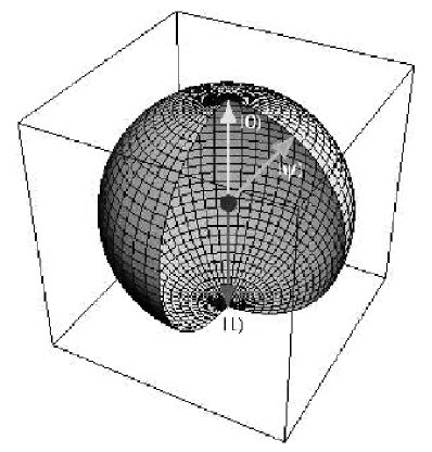
Figure 5.1: Representation of a qubit as a Bloch sphere. Any state of a qubit $|\psi\rangle=\cos(\theta)|0\rangle+e^{i\phi}\sin(\theta)|1\rangle$ corresponds to a point in the so called Bloch sphere $S^{2}$. The states $|0\rangle$ and $|1\rangle$ are localized in the poles. See text for details.

$$\rho\,=\,\frac{1}{2}\big{[}I+{\bf r\sigma}\big{]}$$ (5.2)

where $I$ is the $2\times 2$ identity matrix, ${\bf r}\in{\cal R}^{3}$ and $\{$$\sigma_{n}$$\}_{n=1}^{3}$ are the Pauli matrices. Gathering two-qubits, we have a two-qubit system.

A pure state $\rho_{AB}=|\psi\rangle_{AB}\langle\psi|$ representing an arbitrary two-qubits system can be written as

$$|\psi\rangle_{AB}\,=\,a|0\rangle_{A}\otimes|0\rangle_{B}+b|0\rangle_{A}\otimes|1\rangle_{B}+c|1\rangle_{A}\otimes|0\rangle_{B}+d|1\rangle_{A}\otimes|1\rangle_{B},$$ (5.3)

with $a,b,c,d\in{\cal C}^{2}$ and $|a|^{2}+|b|^{2}+|c|^{2}+|d|^{2}=1$. From now on we omit the tensor product symbol between kets and the subscript referring to which system they belong (e.g. $|0\rangle|1\rangle\equiv|0\rangle_{A}\otimes|1\rangle_{B}$). The definition of entanglement for pure states is particularly simple: after Schmidt-decomposing (5.3) into (4.3) with rank $k$ and coefficients $\{$$w_{i=1..k}$$\}$, entanglement is defined as the Shannon entropy of $\{$$w_{i=1..k}$$\}$ squared. Thus, a state is separable if $k=1$ (zero entropy).

An alternative way of describing the entanglement of a pure state of two-qubits is the following. Consider the total density matrix $\rho_{AB}=|\psi\rangle_{AB}\langle\psi|$. By the action of partial tracing we eliminate the degrees of freedom of either subsystem and end up with a reduced or marginal density matrix (e.g. $\rho_{A}=$Tr_B($\rho_{AB}$)= $\langle 0_{B}|\rho_{AB}|0_{B}\rangle$+$\langle 1_{B}|\rho_{AB}|1_{B}\rangle$). The entanglement $E$ of $\rho_{AB}$ is then defined as the von Neumann entropy of $\rho_{A}$, $E\equiv S(\rho_{A})=-$Tr($\rho_{A}\,\log\rho_{A}$). In point of fact, it is not difficult to see that $S(\rho_{A})=S(\rho_{B})$, as it should be for symmetry reasons. The logarithm of the von Neumann entropy is taken is base 2 ($\log_{2}$) such that maximum entanglement corresponds to 1.

A very interesting family of bipartite pure states is constituted by the so called Bell states. The Bell states correspond to pure states with maximal entanglement and are defined, up to a global phase, as

$$|\Phi^{\pm}\rangle = \frac{1}{\sqrt{2}}(|00\rangle\pm|11\rangle),$$ (5.4)

$$|\Psi^{\pm}\rangle = \frac{1}{\sqrt{2}}(|01\rangle\pm|10\rangle),$$ (5.5)

where $|\Psi^{-}\rangle$ is nothing but the singlet state of two $\frac{1}{2}$-spins. These states have lots of theoretical and practical uses, as we shall see. They are synonymous with EPR states, named after Einstein, Podolsky and Rosen (see Appendix A). As a matter of fact, our “entanglement ruler” could be defined as the quantum correlations contained in the antisymmetric singlet state $|\Psi^{-}\rangle$. Indeed, its entanglement $E$ is maximum ($E(|\Psi^{-}\rangle\langle\Psi^{-}|)=1$).

Mixed states and their entanglement

Pure states are difficult to obtain in the laboratory and hard to store for long periods of time. Due to the interaction with the environment ${\cal E}$, they rapidly spread (decoherence time) into an statistical mixture of different available pure states (a mixed state). In a way, it is more natural to think of entangled mixed states rather than entangled pure states. Actually, if $|\psi_{S}\rangle$ is our initial pure state of the system at $t=0$, the environment described by the state $|{\cal E}\rangle$ dilutes the individuality of $|\psi_{S}\rangle$ into some new state $|\psi_{SE}\rangle$ at $t=T$. Mathematically, $|\psi_{S}\rangle\otimes|{\cal E}\rangle(t=0)\rightarrow|\psi_{SE}\rangle(t=T)$, wherefrom if one could trace out the degrees of freedom of the environment, we would end up with the state of the system at $t=T$ ($\rho_{S}=$Tr_E($|\psi_{SE}\rangle\langle\psi_{SE}|$)). The characterization of entangled mixed states is also necessary for the study of the entanglement properties of pure states of multipartite systems with more than two components. For instance, let us consider a pure state $|\psi_{ABC}\rangle$ of a system with three subsystems A, B, and C. If we want to know the amount of entanglement present between subsystems say A and B, we have to consider the state $\rho_{AB}=$Tr_C($|\psi_{ABC}\rangle\langle\psi_{ABC}|$) which is, in general, mixed.

The complete characterization of mixed two-qubits states requires $4^{2}-1=15$ real parameters. This is so because $\rho$ is a $4\times 4$ hermitian, positive semidefinite matrix ($\rho=\rho^{{\dagger}}$), which implies that $N^{2}$ real entries are needed. The requirement of normalization Tr($\rho$)$=1$ reduces the number to $N^{2}-1$. This is the most general structure of the space of two-qubits given in the so called computational basis ($|00\rangle,|01\rangle,|10\rangle,|11\rangle$). Because a mixed state can be prepared in infinitely many ways, some other decompositions can be more or less interesting depending on the context:

• Sometimes it is useful to decompose a given mixed state in the form of a superposition of Bell states (Bell states form an ortonormal basis). A subclass of these states are named Bell diagonal states, and are written as the convex sum

  $$\rho\,=\,p_{1}|\Psi^{-}\rangle\langle\Psi^{-}|+p_{2}|\Psi^{+}\rangle\langle\Psi^{+}|+p_{3}|\Phi^{+}\rangle\langle\Phi^{+}|+p_{4}|\Phi^{-}\rangle\langle\Phi^{-}|.$$ (5.6)

  The entanglement properties of these states are easy to describe, as we shall see. They appear quite often in quantum teleportation. One such example of Bell diagonal state is given by the so called “Werner states” $\rho_{W}$. The Werner density matrix reads

  $$\rho_{W}\,=\,x|\Phi^{+}\rangle\langle\Phi^{+}|\,+\,\frac{1-x}{4}I,$$ (5.7)

  where $|\Phi^{+}\rangle$ is a Bell state (maximally entangled). $\rho_{W}$ is a mixture of a Bell state, usually a singlet, with the remaining states. The state (5.7) is separable (unentangled) for the mixing coefficient $x\leq 1/3$ [42]. For $x>1/3$ they are entangled and violate the CHSH inequality for $x>1/\sqrt{2}$ [148, 149]. We see that Werner states are mixtures of noise and a maximally entangled state, and therefore, for values of the mixing parameter $x>1/3$ they are entangled and exhibit non-classical features [148, 149]. The fact that Werner density matrices violate the CHSH Bell inequality (when each of the two concomitant subsystems is subjected to a single ideal measurement) for $x>1/\sqrt{2}$, but being entangled, motivated Werner himself to provide a hidden variable simulation of these correlations [42]. The Werner state (5.7) is very popular in the literature. For instance, we have shown [150] that there is a one-to-one correspondence between Werner states and the Heisenberg anti-ferromagnet thermal states of two spinors (two qubits), that is, $\rho(T)=\exp(-H/k_{B}T)/Z(T)$ with $H$ being the Heisenberg Hamiltonian.

• There exists a more pedagogical way of presenting two-mixed states which owes much of its simplicity to the use of Pauli matrices. Resembling Eq. (5.2) for one qubit, any given two-qubits state can decomposed in the following way:

  $$\rho\,=\,\frac{1}{4}\big{[}I\otimes I+{\bf r\sigma}\otimes I+I\otimes{\bf s\sigma}+\sum_{m,n=1}^{3}t_{m,n}\sigma_{n}\otimes\sigma_{m}\big{]}$$ (5.8)

  where $I$ is the identity matrix, ${\bf r,s}\in{\cal R}^{3}$, $\{$$\sigma_{n}$$\}_{n=1}^{3}$ are the Pauli matrices, and $t_{m,n}=$Tr($\rho\,\sigma_{n}\otimes\sigma_{m}$) are the coefficients of a real matrix. The state (5.8) is written in such a way that all non-local terms are contained in the last addend. All quantum correlations present in the mixed state appear due to this last term, while all the others refer to local addressings. Notice that we still need 15 real parameters. This form is specially suitable in the field of quantum optics and quantum tomography.

Nevertheless, when we study global properties of the set of all states ${\cal S}$ we use the generic form in the computational basis. The quantification of entanglement for mixed states is much more difficult than for pure states. Due to this fact, several measures of entanglement that recover the usual one for pure states had been advanced. A concise study is done in the following sections. Also, a thorough exposition of the space of two-qubits and entanglement is drawn in Chapter 8.

5.1.2 Multipartite entanglement

Contrary to what may seem an exception, multipartite entanglement is the rule. The outcome of many parties in mutual interaction result in a statistical matrix $\rho$ that, if entangled, cannot be decomposed as a mixture of product states of the individual subsystems. Nevertheless, at present we have only partial knowledge of the complete picture of multiparticle entanglement. For instance, several quantum algorithms require two registers, that is, two bunches of qubits, to be entangled and this feature is essential for quantum computation. This latter case, however, only requires entanglement of multipartite pure states. A much more difficult problem consists in the classification of multipartite mixed states, which is still under current study.

Historically, the interest in entanglement between more than two parties was motivated by the fact that that correlations among more than two particles present novel and highly nontrivial features not present in states of two particles. This fruitful path was opened by the seminal paper by Greenberger, Horne, and Zeilinger [151]. Here we present a brief sketch of the GHZ experiment. Let us take three well-separated parties $A$, $B$ and $C$, each one of those having two observables $X$ and $Y$, which can adopt the discrete values $\{$$\pm 1$$\}$ only. Let us suppose that we perform three measurements 1, 2 and 3, where in each experiment we measure either $X$ ($m_{x}$) or $Y$ ($m_{y}$) for every party, as arranged in Table 5.1.

	A	B	C	product
1	$m_{x}$	$m_{y}$	$m_{y}$	$r_{1}$
2	$m_{y}$	$m_{x}$	$m_{y}$	$r_{2}$
3	$m_{y}$	$m_{y}$	$m_{x}$	$r_{3}$
$X-$result	$m^{A}_{x}m^{A}_{y}m^{A}_{y}=m^{A}_{x}$	$m^{B}_{y}m^{B}_{x}m^{B}_{y}=m^{B}_{x}$	$m^{C}_{y}m^{C}_{y}m^{C}_{x}=m^{C}_{x}$	$r_{1}r_{2}r_{3}$

Table 5.1: Scheme for the GHZ experimental setting.

The last column reports the product of the outcomes of the different parties. The last row shows the results of the product of the outcomes of the individual measurements (note that $(m^{\mu}_{y})^{2}=1\leavevmode\nobreak\ \forall\mu$). One then should expect that $r_{1}r_{2}r_{3}$ be equal to $m^{A}_{x}m^{B}_{x}m^{C}_{x}$. Let us go to the laboratory and prepare three photons in the state

$$|GHZ\rangle\,=\,\frac{1}{\sqrt{2}}(|000\rangle-|111\rangle),$$ (5.9)

where $|0\rangle$ or $|1\rangle$ may denote opposite states of polarization of a photon. Suppose that we perform, in analogy with the $r_{i}$ results, the following measurements ((5.9) is an eigenstate of these operators)

$$\sigma^{A}_{x}\sigma^{B}_{y}\sigma^{C}_{y}\,|GHZ\rangle = +1\,|GHZ\rangle$$

$$\sigma^{A}_{y}\sigma^{B}_{x}\sigma^{C}_{y}\,|GHZ\rangle = +1\,|GHZ\rangle$$

$$\sigma^{A}_{y}\sigma^{B}_{y}\sigma^{C}_{x}\,|GHZ\rangle = +1\,|GHZ\rangle,$$ (5.10)

we therefore expect $\sigma^{A}_{x}\sigma^{B}_{x}\sigma^{C}_{x}|GHZ\rangle$ to be $(+1)(+1)(+1)=+1$, but if we check the experimental results, we find $\sigma^{A}_{x}\sigma^{B}_{x}\sigma^{C}_{x}|GHZ\rangle=-1\,|GHZ\rangle$ instead! The contradiction with the “expected” value expresses the fact that the GHZ state (5.9) is an entangled state of three particles. Any separable state of the form $|\psi^{A}\rangle\otimes|\psi^{B}\rangle\otimes|\psi^{C}\rangle$ would comply with the value predicted by a local variable theory. It is a kind of Bell theorem without inequalities: superposition exists and properties are not sharp (one cannot attribute properties before measurement, that is why $r_{1}r_{2}r_{3}$ does not equal $m^{A}_{x}m^{B}_{x}m^{C}_{x}$).

Already in the simplest extension of a bipartite system of two qubits, that is, a three qubit system, the characterization of entangled states (pure or mixed) is not an easy task. Even the detection of entanglement is not clear. However, classes of multipartite pure states are known [152] such as

$$|GHZ\rangle = \frac{1}{\sqrt{2}}(|000\rangle-|111\rangle)$$

$$|W\rangle = \frac{1}{\sqrt{3}}(|001\rangle+|010\rangle+|100\rangle)$$

$$|B\rangle = |\Psi^{+}_{AB}\rangle\otimes|0_{C}\rangle$$

$$|S\rangle = |\psi^{A}\rangle\otimes|\psi^{B}\rangle\otimes|\psi^{C}\rangle,$$ (5.11)

where $|B\rangle$ correspond to biseparable states and $|S\rangle$ belong to the class of product states (ergo separable). In the class $|B\rangle$ one can encounter for instance that A(BC) and (AB)C partitions are separable, while (AC)B is entangled! Another interesting example is provided by the complementary state to the so called SHIFTS UPB tripartite mixed state introduced in [153]. Given the set SHIFTS UPB of product states $|\psi_{i}=\{|0,1,+\rangle,|1,+,0\rangle,|+,0,1\rangle,|-,-,-\rangle\}$, with $|\pm\rangle=(|0\rangle\pm|1\rangle)/\sqrt{2}$, one defines its complementary state

$$\rho\,=\,\frac{1}{4}\bigg{(}1\,-\,\sum_{i=1}^{4}|\psi_{i}\rangle\langle\psi_{i}|\bigg{)}.$$ (5.12)

According to [153], state (5.12) has the curious property that it is not only two-way PPT, but also two-way separable, which means that (5.12) has got genuine tripartite mixed entanglement.

In the case of pure states of three qubits, a pioneer result [154] in the description of entanglement in many systems states the “monogamy of entanglement”. That is, for a certain bipartite entanglement measure $E$ and a given system composed by three qubits A, B and C, it is found that

$$E[\rho_{AB}]\,+\,E[\rho_{AC}]\leq E[\rho_{A(BC)}],$$ (5.13)

where $\rho_{AB}=$Tr_C($|\Psi\rangle_{ABC}\langle\Psi|$) and $\rho_{A(BC)}=$Tr_BC($|\Psi\rangle_{ABC}\langle\Psi|$) are the concomitant reduced density matrices. The result (5.13) is conjectured to hold in for arbitary number of qubits. A more detailed account is given in Chapter 11.

In general terms, the characterization of multipartite entanglement is an open question, at least in the terms of the mathematical problem of separability (5.1). When more than two parties are involved, the notion of partitions of the system has to be taken into account, which induces a certain arbitraricity in a rigorous definition of entanglement.

5.1.3 Physically motivated entanglement measures. General properties

Bearing in mind the aforementioned problem of the lack of a general and complete description of the entanglement present in many-body systems, next we give an account of several well known bipartite entanglement measures. To start with, let us investigate some properties of the already used von Neumann entropy (of a subsystem) as a measure of the quantal correlations $E(|\Psi\rangle)$ present in a pure state $|\Psi\rangle$. One such characteristic is that $E(|\Psi\rangle)$ is invariant under local unitary transformations $U=U_{A}\otimes U_{B}$. That is, $E(|\Psi^{\prime}\rangle=U|\Psi\rangle)=E(|\Psi\rangle)$. In other words, $E(|\Psi\rangle)$ cannot increase under LOCC. Thus, one of the many features required by a proposed entanglement measure is that it cannot increase under the action of local operations. In point of fact, the fundamental property is that entanglement between two systems cannot be increased without quantum interaction between them. If the systems are spatially separated, then entanglement between the quantum systems is only allowed to decrease under LOCC. A good source on entanglement measures can be found in [155].

The basic postulates or properties that a reasonable measure of entanglement must exhibit can be summarized as follows.

• 1) For any separable state $\rho_{sep}$ the entanglement measure should be null

  $$E(\rho_{sep})\,=\,0.$$ (5.14)

• 2) The entanglement of a state $\rho$ must remain invariant under local unitary transformations $U=U_{A}\otimes U_{B}$,

  $$E(\rho)\,=\,E(U\,\rho\,U^{{\dagger}}).$$ (5.15)

  It is equivalent to say that a change in the two local basis (associated with each of the two subsystems) upon which states $\rho$ are decomposed must not neither augment nor diminish the entanglement. Besides, any LOCC operation $\Lambda$ should at most leave the entanglement of $\rho$ untouched: $E(\Lambda(\rho))\leq E(\rho)$.

• 3) Suppose that a LOCC operation action on $\rho$ is capable of transforming our initial state into a series of possible final states $\{$$\rho_{f}^{(i)}$$\}$ (an ensemble), each one of those with probability $p_{i}$. We then require

  $$E(\rho)\,\geq\,\sum_{i}p_{i}\,E(\rho_{f}^{(i)}).$$ (5.16)

  This last condition is strongly related to the purification procedure of extracting pure maximally entangled states out of a noisy state $\rho$. Also, we must require a good measure $E$ to be a convex function, $E\big{(}\sum_{i}p_{i}\rho_{i}\big{)}\leq\sum_{i}p_{i}E(\rho_{i})$.

• 4) Once we gather together two entangled non-interacting states $\rho_{1}$ and $\rho_{2}$ in the form $\rho_{1}\otimes\rho_{2}$, we must have that

  $$E(\rho_{1}\otimes\rho_{2})\,=\,E(\rho_{1})+E(\rho_{2}).$$ (5.17)

As we can see, most of these conditions form a set of statements that linger around the notion that entanglement is something that cannot be created or prepared locally, and therefore different local, linear manipulations of states can only diminish – never increase – the “quantity” of quantum correlations.

In the case where $\rho$ corresponds to the density matrix of a pure state, all measures must recover the von Neumann entropy of the reduced density matrix $S(\rho_{A})=-$Tr($\rho_{A}\log_{2}\rho_{A}$), which complies with these demandings. The problem arises in the case of mixed states. There are not many measures that observe the aforementioned demands. One then can either extend the definition for pure states to mixed states $\rho$ by performing a minimization over all possible decompositions of $\rho$ (what is known as a convex roof procedure) or introduce some new measure based on distances between states (distance-based measures), which can relax (not always) some postulate of the previous list.

A. Entanglement of distillation, entanglement cost and entanglement of formation

Suppose that two parties $A$ and $B$ share $N$ pairs of pure states of the form $\psi=a|00\rangle+b|11\rangle$, with $a,b\in{\cal R}$ and $a^{2}+b^{2}=1$ without loss of generality. It is known that these states are partially entangled, because maximum entanglement occurs for $a=b=\frac{1}{\sqrt{2}}$. Imagine that both parties would like to convert these entangled states $\psi^{\otimes N}$ to a smaller supply of $M$ singlet states $\Psi^{-}$, which are maximally entangled. This process is known as distillation of entanglement. In other words, entanglement is concentrated in fewer pairs. Fig.5.2 provides an sketch of the situation. By acting under LOCC operations, one may wonder what is the yield $\frac{M}{N}$. This is the starting point for defining the entanglement of distillation or distillable entanglement of $\psi$, $D(\psi)$

$$Sup._{LOCC}\lim_{N\to\infty}\frac{M(N)}{N}\equiv D(\psi).$$ (5.18)

For pure states, it can be shown that $D(\psi)=S(\rho_{A})$. It gives us the number of units of singlets that can be distilled out of a given state $\psi$.

$\parbox{51.21504pt}{$\rho^{\otimes N}$ \\ pairs}\kern-17.07164pt\left\{\begin{array}[]{l}$$A\,\,\,\,\,\,\,\,\,\,\,\,\,\,\,\,\,\,\,\,\,\,\,\,\,\,\,\,\,\,\,\,\,\,B$$\\ $$\bullet\smile\!\!\frown\!\!\smile\!\!\frown\!\!\smile\!\!\frown\!\!\smile\!\!\frown\bullet$$\\ $$\bullet\smile\!\!\frown\!\!\smile\!\!\frown\!\!\smile\!\!\frown\!\!\smile\!\!\frown\bullet$$\\ $$\bullet\smile\!\!\frown\!\!\smile\!\!\frown\!\!\smile\!\!\frown\!\!\smile\!\!\frown\bullet$$\\ $$\bullet\smile\!\!\frown\!\!\smile\!\!\frown\!\!\smile\!\!\frown\!\!\smile\!\!\frown\bullet$$\\ $$\bullet\smile\!\!\frown\!\!\smile\!\!\frown\!\!\smile\!\!\frown\!\!\smile\!\!\frown\bullet$$\\ .\\ .\\ .\\ $$\bullet\smile\!\!\frown\!\!\smile\!\!\frown\!\!\smile\!\!\frown\!\!\smile\!\!\frown\bullet$$\\ $$\bullet\smile\!\!\frown\!\!\smile\!\!\frown\!\!\smile\!\!\frown\!\!\smile\!\!\frown\bullet$$\end{array}\right.\quad\begin{array}[]{c}{\rm L\ O\ C\ C}\\ {\rm operations}\\ \\ \Longrightarrow\\ \\ \\ \\ \\ \end{array}\quad\left.\begin{array}[]{r}$$A\,\,\,\,\,\,\,\,\,\,\,\,\,\,\,\,\,\,\,\,\,\,\,\,\,\,\,\,\,\,\,\,\,\,B$$\\ $$\bullet\backslash\!/\!\backslash\!/\!\backslash\!/\!\backslash\!/\!\backslash\!/\!\backslash\!/\!\backslash\!/\!\backslash\!/\bullet$$\\ $$\bullet\backslash\!/\!\backslash\!/\!\backslash\!/\!\backslash\!/\!\backslash\!/\!\backslash\!/\!\backslash\!/\!\backslash\!/\bullet$$\\ .\\ .\\ $$\bullet\backslash\!/\!\backslash\!/\!\backslash\!/\!\backslash\!/\!\backslash\!/\!\backslash\!/\!\backslash\!/\!\backslash\!/\bullet$$\\ $$\bullet\backslash\!/\!\backslash\!/\!\backslash\!/\!\backslash\!/\!\backslash\!/\!\backslash\!/\!\backslash\!/\!\backslash\!/\bullet$$\\ \end{array}\right\}\hskip 2.84526pt\parbox{51.21504pt}{$(\Psi^{-})^{\otimes M}$}$

Figure 5.2: Distillation of entanglement.

The reverse process is called dilution of entanglement. Starting from $M$ singlets, $N$ copies of the state $\psi$ are obtained under LOCC operations, defining the entanglement cost $E_{C}(\psi)$

$$Sup._{LOCC}\lim_{N\to\infty}\frac{M(N)}{N}\equiv E_{C}(\psi).$$ (5.19)

Also for pure states, $E_{C}(\psi)=S(\rho_{A})$. Thus, we have that both distillation and dilution of entanglement are equal and reversible asymptotically. The proof that $D(\psi)$ equals the reduced von Neumann entropy $S(\rho_{A})$ is not difficult, but tedious. It basically consists in expanding the general form of $\psi^{\otimes N}$. After assuming that the unit of entanglement is given by the entanglement of the singlet state and some asymptotic approximation is made, it is seen that $E(\psi)\sim NS(\rho_{A})$, for $N\rightarrow\infty$. The formal proof of $E_{C}(\psi)=S(\rho_{A})$ is a bit more involved, and can be performed with the aid of the theory of generalized measurements.

It is also important to stress that the above procedure of distillation is reversible, but this is not the case for mixed states, where both entanglement of distillation and entanglement cost differ from each other. This is an important issue: there appears an intrinsic irreversibility feature in passing from pure to mixed states: the so called bound entangled states are so thoroughly mixed that cannot be distilled. This fact has indeed led to conjecture some connection between the theory of entanglement and the Second Law, as discussed in forthcoming sections.

Now then, how can we define a measure of entanglement for mixed states? If we agree that the reduced von Neumann entropy is a good measure of entanglement for pure states, it is somewhat natural to extend this definition to mixed states. One way to do so is by doing the convex roof

$$E(\rho)\,=\,inf\,\sum_{i}p_{i}E(|\psi\rangle\langle\psi|),$$ (5.20)

with $\sum_{i}p_{i}=1$ and $0\leq p_{i}\leq 1$. The minimum is taken over all possible decompositions of the mixed state $\rho=\sum_{i}p_{i}|\psi\rangle\langle\psi|$ into pure states (which need not be orthogonal). This huge task of optimizing (5.20) is still an open problem, but luckily for us there exists a closed formula for the two-qubits instance, which results in the physically motivated measure of entanglement provided by the entanglement of formation $E_{F}$ [157, 158]. This measure quantifies the resources needed to create a given entangled state $\rho$. That is, $E_{F}(\rho)$ is equal to the asymptotic limit (for large $N$) of the quotient $\frac{M}{N}$, where $M$ is the number of singlet states needed to create $N$ copies of the state $\rho$ when the optimum procedure based on local operations is employed. This procedure goes in the opposite direction to the one sketched in Fig.5.2. The relationship between the entanglement of formation $E_{F}$ and the entanglement cost $E_{C}$ in the case of mixed states remains and open question. That is, it is not known if $E_{F}=E_{C}$ in the general mixed-state case, as it is for pure states.

The entanglement of formation for two-qubit systems is given by Wootters’ expression [158]

$$E[\rho]\,=\,h\left(\frac{1+\sqrt{1-C^{2}}}{2}\right),$$ (5.21)

where

$$h(x)\,=\,-x\log_{2}x\,-\,(1-x)\log_{2}(1-x),$$ (5.22)

and the concurrence $C$ is given by

$$C\,=\,max(0,\lambda_{1}-\lambda_{2}-\lambda_{3}-\lambda_{4}),$$ (5.23)

$\lambda_{i},\,\,\,(i=1,\ldots 4)$ being the square roots, in decreasing order, of the eigenvalues of the matrix $\hat{\rho}\tilde{\rho}$, with

$$\tilde{\rho}\,=\,(\sigma_{y}\otimes\sigma_{y})\rho^{*}(\sigma_{y}\otimes\sigma_{y}).$$ (5.24)

The above expression has to be evaluated by recourse to the matrix elements of $\hat{\rho}$ computed with respect to the product basis. $C^{2}$ can be regarded as a proper measure of entanglement, as (5.21) is a monotonic increasing function of $C^{2}$. For pure states (5.21) reduces to the usual von Neumann entropy. As a matter of fact, $C^{2}=4\,$det$\rho_{A}$ for pure two-qubits states. The general form for a bipartite pure state [159] $|\psi\rangle\in{\cal H}_{N}\otimes{\cal H}_{K}$ is ($N\leq K$ is assumed) $C(|\psi\rangle)=\sqrt{2[|\langle\psi|\psi\rangle|^{2}-Tr(\rho_{N}^{2})]}$, with $\rho_{N}=$Tr${}_{K}(|\psi\rangle\langle\psi|)$. Although there is no general expression for the concurrence of mixed bipartite states, F. Mintert et al. derive in [160] a lower bound for the concurrence of mixed bipartite quantum states, valid in arbitrary dimensions.

In the case of Bell diagonal states $\rho$ (5.6), which appear quite often in quantum teleportation and quantum cryptography scenarios, the concurrence reads $C=2\lambda_{m}-1$, where $\lambda_{m}$ is the maximum eigenvalue of $\rho$. Thus, for this family of states, it suffices to say that a given state is entangled if $\lambda_{m}\geq\frac{1}{2}$.

B. Robustness of entanglement

A nice measure is provided by the robustness of entanglement [161]. Given an entangled state $\rho$ and separable state $\rho_{s}$, a new density matrix $\rho(s)$ can be constructed as

$$\rho(s)=\frac{1}{s+1}(\rho+s\rho_{s}),\quad s\geq 0.$$ (5.25)

The ensuing state $\rho(s)$ can be either separable or entangled. What is certain is that there always exits a minimal ${\bf s}$ corresponding to $\rho_{s}$ such that $\rho(s)$ is separable. This optimal value ${\bf s}$ is called the robustness of $\rho$ with respect to $\rho_{s}$, and expressed as $R(\rho\parallel\rho_{s})$. The inferior of all optimal values is known as the absolute robustness of $\rho$, or simply the robustness of entanglement

$$R(\rho\parallel S)\equiv\min_{\rho_{s}\in S_{sep}}R(\rho\parallel\rho_{s}),$$ (5.26)

where the whole set of separable states ${\cal S}_{sep}$ is explored. This measure is based on a simple physical operation: mixing with locally prepared states, and certainly it does not increase under LOCC operations. It admits the geometrical interpretation of the minimal distance of the entangled state $\rho$ to the boundary of the set ${\cal S}_{sep}$.

The robustness of entanglement can be computed analytically for pure states. Recalling the Schmidt decomposition (4.3) for a pure state in a system ${\cal H}_{N}\otimes{\cal H}_{M}$, with $K=$min$(N,M)$ being the rank of the state and coefficients $\{$$w_{i}$$\}_{1}^{K}$, $R(\rho\parallel S)=\big{(}\sum_{i=1}^{K}w_{i}\big{)}^{2}-1$. There is no general expression, to our knowledge, even for the bipartite case of two-qubits systems. However (5.26) is not difficult to compute numerically taking advantage of the fact that ${\cal S}$ is a convex and compact set.

C. Relative entropy of entanglement and similar measures

The relative entropy measure belongs to the class of entanglement measures that are based on distances between states. It need not has to be a proper metric is the space of all states ${\cal S}$, and in fact it is not, but it can be extended to recognized metrics in that space ${\cal S}$. The relative entropy of formation is defined as [163]

$$E^{rel}[\hat{\rho}]\,\equiv\,min_{\sigma\in{\cal S}_{sep}}\,D(\rho||\sigma),$$ (5.27)

where the minimum is taken over all possible states $\sigma$ that are unentangled (set ${\cal S}_{sep}$), and $D$ is the quantum version of the Kullback-Leibler relative entropy[164] $S^{rel}(\rho||\sigma)=$Tr$\left(\rho\log\rho-\rho\log\sigma\right)$. The measure (5.27) can be interpreted as the minimum distance from the set ${\cal S}$ when one uses $S^{rel}(\rho||\sigma)$ as a ruler. Besides, measure (5.27) acquires a well-defined statistical meaning, in terms of the quantum Sanov’s Theorem [87]: the probability of not distinguishing two quantum states $\sigma$ and $\rho$ after $n$ measurements is

$$p(\rho\rightarrow\sigma)\,=\,e^{-n\,S(\sigma||\rho)}.$$ (5.28)

In this context the situation deals with the probability of mistaken an entangled state from a disentangled one.

This measure possesses some similarities with the robustness of entanglement (5.26): they are both taken as minima of quantities representative of the entangled state $\rho$ with respect to ${\cal S}_{sep}$, and the two of them are easy to extend to arbitrary number of parties and dimensions. However, (5.27) reduces to the von Neumann entropy of entanglement for pure states, while this is not the case for (5.26). The relative entropy fulfils the requirement of a “decent” entanglement measure. There exists only one serious drawback, though: it can only be computed analytically for Bell diagonal states (5.6). However, convexity of ${\cal S}_{sep}$ again allows us to numerically compute [165] the quantity (5.27).

Other measures for $D(\rho||\sigma)$ can be used instead of $S^{rel}(\rho||\sigma)$. In point of fact, the latter expression is not a true metric simply because it is not symmetric. Therefore one could in principle use some metric distance to be minimized, such as the Bures or Hilbert-Schmidt distances [166] between states, but they do not incorporate the von Neumann entropy of entanglement for pure states.

5.2 Entanglement for indistinguishable particles

So far we have delt with entanglement for distinguishable particles, assuming that a qubit or a qudit (coherent superposition of $D$ states) is encoded in the degrees of freedom of that particle. Examples of this situation could be the spin degrees of freedom of a spin-$s$ particle ($2s+1$), the $D$ relevant energy levels of an atom, or the polarizations of a photon. Speaking of qubits, we have implicitly supposed that the $N$ parties possess identical qubits (encoded in identical particles), but this is not at all the general framework. We could easily create an entangled state of two-qubits where the two important energy levels are encoded in each one of two perfectly distinguishable atoms, say Rubidium and Calcium. In this picture of entanglement, the distinction of states as tensor products is perfectly licit. Even in the case where the particles (representing the qubits) are identical, this picture preserves its validity because the systems are well-located and far apart from each other, so that the intrinsic correlations – which are always present – due to the statistics of identical particles is practically negligible for all practical purposes.

Now let us tackle the problem of entanglement between identical particles where the overlap of the wavefunctions is neither zero nor negligible. This is a typical situation encountered in the proposals of quantum gates for quantum computation based on the present semiconductor technology (see [167] and references therein). It is possible nowadays to confine a well defined number of electrons in quantum dots. Even for the simple case of two quantum dots confining one electron per site, the global wave function $|\Psi\rangle_{AB}$ has to be properly antisymmetrized unless they do not interact by any means. As soon as the electrons start to “see” each other, we can no longer describe the concomitant Hilbert space ${\cal H}$ as a tensor product of individual subspaces ${\cal H}_{A}$,${\cal H}_{B}$. Let us consider the case of two identical fermions (bosons receive similar a treatment) in an $N$-dimensional single particle space ${\cal H}_{N}$, where the total Hilbert space corresponds to ${\cal A}({\cal H}_{N}\otimes{\cal H}_{N})$ with ${\cal A}$ being the antisymmetrization operator. Under this conditions, an arbitrary state can be written as

$$|w\rangle=\sum_{i,j=1}^{N}w_{ij}f^{\dagger}_{i}f^{\dagger}_{j}|vacuum\rangle,$$ (5.29)

where $f^{\dagger}_{i}$ are the fermionic creation operators, and the antisymmetric matrix $w_{ij}$ fulfils the normalization condition Tr$(w^{*}w)=-1/2\,$. The cases of pure and mixed two-fermion states have been studied in [168] and an extension of the concurrence measure (5.23) is given.

• i) Pure states. Rotating appropriately the state basis of a two-fermion state $|w\rangle$ we obtain

  $$|w\rangle=2\sum_{k=1}^{m}r_{k}f^{\dagger}_{2k}f^{\dagger}_{2k-1}|vacuum\rangle,$$ (5.30)

  with $2m\leq N$ and $r_{k}$ real and positive. Regarding each term as an Slater determinant, $|w\rangle$ has a minimal number $m$ of Slater determinants, in analogy with the Schmidt rank (4.3). In this case ($N=2\times 2=4$) the concurrence $C(|w\rangle)$ is defined as

  $$C(|w\rangle)=\Big{|}\frac{1}{2}\sum_{i,j,k,l=1}^{4}\epsilon^{ijkl}w_{ij}w_{kl}\Big{|},$$ (5.31)

  where $\epsilon$ is the usual antisymmetric tensor.

• ii) Mixed states. Let $\rho=\sum_{i}p_{i}|w_{i}\rangle\langle w_{i}|$ be a given mixed two-fermion state. Defining $|\widetilde{w}_{i}\rangle=\sum_{i,j,k,l=1}^{4}\epsilon^{ijkl}w_{kl}f_{i}^{\dagger}f_{jl}^{\dagger}|vaccum\rangle$, $\tilde{\rho}=\sum_{i}p_{i}|\widetilde{w}_{i}\rangle\langle\widetilde{w}_{i}|$ and $\lambda_{i}$ as the eigenvalues (real and positive) of $\rho\tilde{\rho}$ in decreasing order, the concurrence for mixed states is constructed as

  $$C(\rho)=\max(0,\lambda_{1}-\sum_{i=2}^{6}\lambda_{i}).$$ (5.32)

  Note the similarities between (5.32) and the definition (5.23) for distinguishable two-qubits. This last definition is obtained as the convex roof of (5.31).

Antisymmetrization, essential whenever we deal with identical (fermionic or bosonic) particles, might lead to misunderstandings as far as entanglement is concerned. This was clearly pointed out in [169]. Suppose that we have the state $|R\rangle=|Me$ exposing $\rangle\otimes|You$ reading $\rangle$ describing two composite systems. From the tensor product structure one judges that this state is separable. The systems need not be identical, but if they do are, we must antisymmetrize the global state even if they are far apart. The ensuing state ${\cal A}|R\rangle$ possesses no entanglement at all because identical particles do not produce entanglement by themselves. On the contrary, a state like $\frac{1}{\sqrt{2}}\big{[}|Me$ exposing $\rangle\otimes|You$ reading $\rangle$ - $|Me$ reading $\rangle\otimes|You$ exposing $\rangle\big{]}$, which is entangled from the very beginning, must remain non-separable after ${\cal A}$.

However, the correlations that arise from the statistics of the particles find interesting applications in quantum information theory. In [170, 171] it is shown that indistinguishability enforces a transfer of entanglement from internal to spatial degrees of freedom of a system without interaction, and an entanglement concentration scheme which uses only the effects of quantum statistics of indistinguishable particles is exposed.

Summing up, the total correlations present in a given state representing the concomitant physical system are the result of the sum of statistical correlations plus quantum correlations, which arise from previous interactions between the constituents of the system. It is difficult to ascertain the feasibility of addressing the latter type of correlations in quantum information, at least experimentally. There might be some reason for choosing distinguishable qubits to the detriment of indistinguishable particles. However, systems of indistinguishable particles possess very interesting features as described in the field of condensed matter. It is in along this line of reasoning that a novel approach to entanglement makes its appearing.

5.3 Relativity of entanglement: a new insight

In the previous case of the problem of indistinguishable particles there are some important difficulties in the partition of the Hilbert space: when adding a particle $s$ to a system of $N$ identical particles, formally one can write the total Hilbert space of the system as ${\cal H}_{N+1}\cong{\cal H}_{N}\otimes h_{s}$, where $h_{s}$ is Hilbert space of $s$. If the particle which is added is identical to the rest of $N$ particles, then this description cannot be possible because it does not take into account the statistics of identical particles, either bosons or fermions. Instead, one has to recall the Fock space of second quantization $\oplus_{N=0}^{\infty}{\cal H}^{(N)}_{F,B}$. It is nothing but the occupation number representation: $({\cal C}^{2})^{\otimes N}$ for fermions and $(h_{\infty})^{\otimes N}$ for bosons, where $h_{\infty}$ spans the harmonic oscillator basis. These considerations led us to Eq. (5.29). However, some paradoxes appear. Suppose that we have a single particle state which can be either in the states $A$ or $B$, similar to two different sites or “parties”. In second quantization, it reads as

$$|\Psi\rangle\,=\,\frac{1}{\sqrt{2}}(c_{A}^{\dagger}+c_{B}^{\dagger})|vacuum\rangle\,=\,\frac{1}{\sqrt{2}}(|1,0\rangle+|0,1\rangle),$$ (5.33)

where $c_{A,B}^{\dagger}$ are the creation operators of sites $A$ and $B$ acting on the vacuum, respectively. This case is illustrative of the fact that even in the case of a single particle, we can have entanglement between its possible modes. This is what is known as the counterpart of “particle entanglement”, wherefrom we now deal with modes. This picture [172] is in some sense complementary to the one presented in the discussion of identical particles. Now, the paradox arises when (5.33) can be transformed into the state $|1,0\rangle$ after a unitary transformation action upon $c_{A,B}^{\dagger}$. How is it possible to convert a maximally entangled state like (5.33) into a separable state like $|1,0\rangle$? The solution consists in differentiating mode from particle entanglement, pointing out that entanglement may not be an absolute quantity. In other words, a state is entangled with respect to which picture you use. This fact induces some loose sense of arbitrarity in the definition of entanglement.

Due to this last consideration, the formal description of the separability problem and, in turn, of entanglement, in terms of (5.1) has been questioned. Zanardi et al. pointed out in [145] that the partition of a quantum system into subsystems is dictated by the set of operationally accessible interactions and measurements available by the observer: “Suppose one is given a four-state quantum system. How does one decide whether such a system supports entanglement or not? In other words, should the given Hilbert space (${\cal C}^{4}$) be viewed as bipartite ($\cong{\cal C}^{2}\otimes{\cal C}^{2}$), or irreducible?” [145].

This idea arises at the same time that a new theory of entanglement is developed in the enlightening work of H. Barnum et al. from the group of Los Alamos [146, 147]. This new theory argues that entanglement is relative to a distinguished subspace of observables (in terms of algebras) rather than a distinguished subsystem decomposition. A new measure of entanglement – the purity $P_{h}$ – is properly introduced. It is remarkable that in this new framework the measure for pure states is recovered under certain conditions of the information available to the observer. As we shall see next, it also finds an exciting place in the description of many-body systems.

5.3.1 The Purity measure $P_{h}$. Mathematical grounds

In this subsection we shall highlight the basics of the mathematical theory of Generalized Entanglement (GE) developed by the group of Los Alamos, together with the concomitant definition of the so called “purity” measure $P_{h}$. It will be necessary to say a few words on Lie algebras, in order to clarify the tenets of GE. Finally, we will establish a link between the purity measure $P_{h}$ and condensed matter theory, through the issue of quantum phase transitions (QPTs).

Let us start by recalling the standard framework for entanglement. Throughout this Chapter and the previous one, devoted to the detection of entanglement, it has become clear that the Hilbert space ${\cal H}$ of a given system may support different tensor product decompositions. In fact, the entanglement of state $\rho$ in ${\cal H}$ is defined once a preferred subsystem decomposition has been chosen (${\cal H}\cong\otimes_{i}\,{\cal H}_{i}$). One interesting feature of entanglement in the usual context is that a pure state $|\Psi\rangle\in{\cal H}$ is entangled iff the state of any of its subsystems is described by a mixed state. In point of fact, if $|\Psi_{AB}\rangle$ happens to be any of the Bell states, which are maximally entangled, it is immediate to obtain that the reduced density matrices $\rho_{A,B}=$Tr${}_{B,A}|\Psi\rangle_{AB}\langle\Psi|$ represent maximally mixed states, and therefore are unentangled states. In other words, entangled pure states look mixed to local observers. This observation will be of crucial importance in the development of a theory of GE.

Usually these decompositions appear naturally in the description of quantum information processing features, because when that parties are well-separated (in real space), one can treat them as distinguishable quantum subsystems. The problem arises in the conflict described previously between particle or mode entanglement, and the question of describing the entanglement of more than two particles, specially crucial in the case of indistinguishable particles.

Entanglement as an observer-dependent concept

The formal theory describing the GE is given in references [146, 147]. Let us recall here the key concepts.

i) The GE is relative to a subspace of observables $\Omega$ of the quantum system.

Let us start with the description of the usual Lie algebra. A Lie algebra $h$ is a vector space endowed with a binary operation or map (the commutator operation) satisfying antisymmetry, and the well-known Jacobi identity. It is said that an ideal $I$ in a Lie algebra is a subalgebra such that for $x\in I$ and arbitrary h $\in h$, $[{\rm h},x]\in I$. A Lie algebra is simple if it contains no proper ideals. The algebra $h$ will be semisimple iff it can be written as a direct sum of simple Lie algebras. Given a semisimple Lie algebra $h$, a maximal commutative subalgebra is known as a Cartan subalgebra $c$ of $h$. If a vector space carries a representation of $h$, then it decomposes into orthogonal joint eigenspaces $V_{\lambda}$ of the operators in $c$, that is, for each $V_{\lambda}$ there exists a set of states $|\psi\rangle$ such that for $x\in c$, $x|\psi\rangle=\lambda(x)|\psi\rangle$ ($\lambda$ is called the weight of $V_{\lambda}$). The space of operators of $h$ orthogonal to $c$ can be classified as raising ($e_{\mu}$) and lowering ($e_{-\mu}$) operators. The set of lowest-weight spaces for all Cartan subalgebras is the orbit of any one such state under the Lie group generated by $h$. These states are the generalized coherent states [146, 147], which can be represented as

$$|GCS\rangle\,=\,e^{\sum_{\mu}(\alpha_{\mu}\,e_{\mu}-\overline{\alpha}_{\mu}\,e_{-\mu})}|ref\rangle,$$ (5.34)

with $|ref\rangle$ being an extremal state (in physical terms, the ground state of a system Hamiltonian, for instance). These generalized coherent states constitute a natural extension of the familiar ones corresponding to the harmonic oscillator.

ii) Extension of the fact that entangled pure states look mixed locally.

The basic idea is to generalize the observation previously made, namely, that pure entangled states possess maximally mixed states when we trace over the degrees of freedom of the rest of the subsystems (reduced state). In other words, they look entangled as a whole, but unentangled locally. Once we are given a pure state and we distinguish a relevant subspace of observables $\Omega$, with respect to which the GE is considered, the associated reduced state is obtained in this framework by only taking into account the expectation values of those $\Omega$-observables. Therefore, we say that a state is generalized unentangled relative to $\Omega$ if its reduced state is pure, and vice versa. Mixed unentangled states are addressed in the usual way (convex combinations of unentangled pure states). One can grasp more physical insight about generalized unentangled states when viewed as the set of states that are unique ground states of a distinguished observable, say a Hamiltonian. The rest of extensions of this theory, such as the generalized LOCC operations can be found in [146, 147].

The Purity measure $P_{h}$

Let us give the definition of the $h$-purity. Let $\{x_{i}\}$ be a Hermitian and normalized orthogonal basis for $h$, that is, $x_{i}^{\dagger}=x_{i}$ and Tr($x_{i}x_{j}$)$\infty\,\delta_{ij}$. For any pure state $|\Psi\rangle\in{\cal H}$, the purity of $|\Psi\rangle$ relative to $h$ is

$$P_{h}(|\Psi\rangle)\,=\,\sum_{i}|\langle\Psi|x_{i}|\Psi\rangle|^{2}.$$ (5.35)

This measure is endowed with a clear geometric meaning: $P_{h}(|\Psi\rangle)$ is the (square) distance from 0 of the projection of $|\Psi\rangle\langle\Psi|$ onto $h$, provided we employ the usual trace inner-product norm. In the case that $h$ is a Lie algebra, the purity measure (5.35) is invariant under group transformations, $\tilde{x}_{i}=g^{\dagger}x_{i}g$, where $g\in e^{i\,h}$. Let us suppose that we have a preferred set of operators $h$, say Hamiltonians for instance. These Hermitian operators may generate a Lie group of unitary operators via $h\rightarrow e^{i\,h}$, or observables.

With this definition of the purity measure $P_{h}$, it is plain that the previous generalized coherent states GCS possess maximal purity, that is, $P_{h}(|GHS\rangle)=1$, because they are already extremal (extremal projection onto $h$) with respect to 0. Therefore, in the framework of GE, the more entangled is a state with respect to some set $h$, the less $h$-purity it possesses, and vice versa. Once the mathematical details of the theory of GE are unfold, they prove the power of the Lie-algebraic setting.

This measure recovers the results obtained in the traditional framework of bipartite entanglement, provided the right set of observables is chosen. The physics behind these formulas is that entanglement is relative to the information (in terms of observables following an algebra) one has access to. On the one hand, in the case of two-spin 1/2 particles, having access to $\Omega=h=su(2)\oplus su(2)=\{S_{x}^{j},S_{y}^{j},S_{z}^{j},j=1,2\}$ give rise to quantum correlations –entanglement– between the spin degrees of freedom of the two particles, that is, a Bell state has zero $P_{h}$. On the other hand, if we have access to all correlations, expressed in the form $\Omega^{\prime}=h^{\prime}=su(4)$, a Bell state will have non-zero $P_{h^{\prime}}$.

The applications of this purity measure can extend to the condensed matter framework. In Chapter 14 we describe how the purity may describe a quantum phase transition, once a proper algebra of observables has been chosen.

5.4 Thermodynamic analogies for entanglement

This section is mainly devoted to the similarities that some authors have established between entanglement and the Laws of Thermodynamics [173]. One must say that entanglement is understood as the usual quantum correlation existing between definite distinguishable parties. The analogy no longer works outside the orthodox view of entanglement exposed in previous sections. Along these lines of reasoning, we clarify some aspects previously discussed regarding some processes involving manipulations of entanglement.

At first sight, the fact that there is a unique measure of entanglement for pure states (the von Neumann entropy of entanglement) shared with its thermodynamical counterpart may point out some connexion between the theory of quantum entanglement and Thermodynamics. Both of them share the historical problem of defining and quantifying the resources in terms of known quantities and brand new ones, such as entropy, which had little intuition by the time of Carnot. Also, strictly speaking we do not handle entanglement, but states that possess entanglement. Starting the analogy, the same situation is encountered in Thermodynamics, where work is the addressed quantity. The conjunction of work and heat (disordered work) boils down to the First Law, the preservation of energy. Irreversibility and reversibility appears in the manipulation of entangled states. We learned that the processes of distillation and dilution of entanglement for pure states are reversible: $E_{D}=E_{C}$, recalling that $E_{D}$ is the asymptotic yield of singletons drawn out of non-maximally pure states, and that $E_{C}$ is the reverse procedure. However, this is not the case for mixed states, where the total entanglement $E$ is imperfectly distilled so that $E_{D}<E_{C}$. This is due to the fact that some entanglement (the so called bound entanglement) can not be distilled. So some “arrow of time” appears in quantum information when dealing with mixed states. It is like there existed two fundamental classes of entanglement, namely, pure state – ordered – and mixed state – disordered – entanglement. Then the process of extracting useful “free” entanglement $E_{free}$ is similar to the one of drawing useful energy (work) between two heat reservoirs. The basic assumption in quantum information that entanglement cannot be created or increased by local operations or classical communications (LOCC) finds its counterpart (first emphasized by Popescu and Rohrlich in [174]) in the Second Law, which asserts that the entropy of a system cannot decrease in a isolated system. Going one step further along this analogy, one could in principle regard the free entanglement $E_{free}$ ($\equiv E_{D}$) as a sort of generic “free” energy $F$ [175], and the total entanglement $E$ as an internal energy $U$, so that $E_{bound}=E-E_{free}\equiv T_{x}S$ (recall $U=F+TS$). Thus, for entangled pure states $T_{x}S=0$, while some undefined “temperature” $T_{x}$ exists for entangled mixed states.

Some may argue that the generalization of the above conclusions to the whole class of states $\rho$ by means of thermodynamic analogies is somewhat risky, precisely because some problems regarding separability remain open still. Furthermore, the analogy with Thermodynamics is by far incomplete (e.g. what is the equivalent of the temperature $T$?). Perhaps the fact that entanglement can be regarded as a resource and that certain manipulations of it are irreversible opened a path for developing some analogy with energy and the way it is manipulated in physics, hence the connection with the First and Second Law. What is certain, however, is that the process of changing pure entanglement into mixed entanglement is irreversible, which makes the distinction between pure and mixed states essential for all practical purposes in quantum information theory.

Part III The role of entanglement in different physical scenarios

Chapter 6 The maximum entropy principle and the “fake” inferred entanglement

The inference of entangled quantum states by recourse to the maximum entropy principle has been considered in the literature [176, 177, 178, 179, 180]. In particular, the question of how to estimate in a reliable way the amount of entanglement of a bipartite quantum system when only partial, incomplete information about its state is available was addressed by Horodecki et al. [176]. Various strategies have been advanced in order to tackle this problem [176, 178, 179, 180, 181]. Horodecki’s question has also been considered in connection with procedures for the entanglement purification of unknown quantum states [182]. The motivation behind these lines of inquiry is the full description of quantum entanglement, which constitutes, as we know, the basic resource required to implement several of the most important processes studied by quantum information theory [110, 114, 115].

If one has enough information it is possible to determine the amount of entanglement of a quantum system even if the available information does not allow for a complete knowledge of the system’s state. An interesting example of this situation was discussed by Sancho and Huelga in [181], where the minimal experimental protocol required for determining the entanglement of a two-qubits pure state from local measurements is exposed. Another important result is that the knowledge of the expectation value of just one observable (local or not) does not suffice to determine the entanglement of a given unknown pure state of two particles. The case in which the prior information is not sufficient for a complete determination of the amount of entanglement was further examined by Horodecki et al. [176]. These authors did not restrict their analysis to pure states. They assumed that the available information consists of the mean values of a given set of observables $\hat{A}_{i}$. Jaynes’ maximum entropy (MaxEnt) principle [8, 9] provides a general inference scheme to treat this kind of situations. According to Jaynes’ principle, one must choose the state yielding the least unbiased description of the system compatible with the available data. That state is provided by the statistical operator $\hat{\rho}_{ME}$ that maximizes the von Neumann entropy $S\,=\,-Tr(\hat{\rho}\,\ln\hat{\rho})$ subject to the constraints imposed by normalization and the expectation values $\langle\hat{A}_{i}\rangle\,=\,Tr(\hat{\rho}\hat{A}_{i})$ of the relevant observables $\hat{A}_{i}$.

Even though Jaynes’ principle does provide a very satisfactory answer in many situations [8, 9], Horodecki et al. [176] showed that the straightforward application of Jaynes’ prescription in its usual form is not always an appropriate strategy for dealing with entangled states. It was shown in [176] that the standard implementation of Jaynes’ principle may create “fake” entanglement. For example, the MaxEnt density matrix may correspond to an entangled state even if there exist separable states compatible with the prior information. Since quantum entanglement is, in many cases, the basic resource needed when processing quantum information, statistical inference procedures that overestimate the amount of available entanglement should be handled with care. Furthermore, it is well-known that local operations and classical communication (LOCC) can never increase the amount of entanglement between remote systems, but they can make it decrease. As a consequence, one should often bet on the decrease of entanglement and not be very “optimistic” when estimating the available amount of this resource. The above considerations suggests that, in order to deal with some situations involving entanglement, the usual form of Jaynes’ prescription needs to be modified or supplemented in an appropriate way. Various such schemes have been proposed. Horodecki et al. [176] proposed a combined strategy based on a constrained minimization of entanglement followed by a maximization of the von Neumann entropy. Alternatively, Abe and Rajagopal [180] explored the possibility of inferring entangled states by recourse to a variational principle based on non-extensive information measures.

So far, the work done in connection with Horodecki’s problem of fake inferred entanglement focused on that particular case in which the prior information is given by the mean value of the Bell-CHSH operator [176, 178, 179, 180]. In this Chapter we explore what happens when the available prior information consists of the expectation value of operators exhibiting a more general form, such as operators diagonal and non diagonal in the Bell basis (5.6), while we provide counterexamples to the general prescription proposed in [179] by Rajagopal for solving the problem of fake entanglement. Finally, for bipartite systems consisting of two qubits, and assuming that we know the expectation value b of the most general operator diagonal in the Bell basis, we explore the whole set of physical states ${\hat{\rho}}$ in the $({\it b},E({\it b}))$-plane, where $E(\hat{\rho})$ is the entanglement of formation (5.21). States that possess the maximum, or the minimum, amount of entanglement are derived explicitly.

6.1 Sketch of Horodecki’s and Rajagopal’s treatment

Following Horodecki et al. let us assume that the prior (input) information is given by the expectation value $b$ of the Bell-CHSH observable [39]

$$\hat{B}=\sqrt{2}\,\Bigl{(}\sigma_{x}\otimes\sigma_{x}+\sigma_{z}\otimes\sigma_{z}\Bigr{)}=2\sqrt{2}\,\Bigl{(}|\Phi^{+}\rangle\langle\Phi^{+}|-|\Psi^{-}\rangle\langle\Psi^{-}|\Bigr{)}\,$$ (6.1)

which is defined in terms of the components of the well-known Bell basis,

$$|\Phi^{\pm}\rangle = \frac{1}{\sqrt{2}}\,\Bigl{(}|00\rangle\pm|11\rangle\Bigr{)},$$ (6.2)

$$|\Psi^{\pm}\rangle = \frac{1}{\sqrt{2}}\,\Bigl{(}|10\rangle\pm|01\rangle\Bigr{)}.$$ (6.3)

The Bell observable is nonlocal. In order to measure the Bell observable one relies upon local operations and classical communication between the parts (that is, LOCC operations). It can not be measured without interchange of classical information (e.g. a telephone call) between the observers [176].

The MaxEnt state obtained by recourse to the standard prescription, when the sole available information is given by $b=\langle\hat{B}\rangle$, is described by the density matrix [176]

$$\hat{\rho}_{ME}(b) = \frac{1}{4}\Bigg{[}\left(1+\frac{b}{\sqrt{2}}+\frac{b^{2}}{8}\right)|\Phi^{+}\rangle\langle\Phi^{+}|+\left(1-\frac{b}{\sqrt{2}}+\frac{b^{2}}{8}\right)|\Psi^{-}\rangle\langle\Psi^{-}|$$ (6.4)

$$+\left(1-\frac{b^{2}}{8}\right)\Bigl{(}|\Psi^{+}\rangle\langle\Psi^{+}|+|\Phi^{-}\rangle\langle\Phi^{-}|\Bigr{)}\Bigg{]}.$$

Rajagopal [179] and Abe and Rajagopal [180] showed that the inclusion of $\sigma^{2}=\langle\hat{B}^{2}\rangle$ within the input data set entails important consequences for the inference of entangled states. The main idea of Rajagopal’s proposal [179] is to consider the density matrix $\hat{\rho}_{MS}$ obtained by considering both mean values $b=\langle\hat{B}\rangle$ and $\sigma^{2}=\langle\hat{B}^{2}\rangle$ as constraints in the MaxEnt prescription, and assuming that the mean value of $\hat{B}^{2}$ adopts the minimum value compatible with the given value of $b$. Rajagopal proved that $\hat{\rho}_{MS}$ is separable if and only if $b<\sqrt{2}$. The method employed by Rajagopal to characterize the states $\hat{\rho}_{MS}$ of minimum-$\sigma^{2}$ rests heavily on the particular form of the Bell operator. A different approach is needed if one wants to implement Rajagopal’s inference scheme when the input information consists of the mean value of more general observables.

The operators $\hat{B}$ and $\hat{B}^{2}$ verify the relations

$$\hat{B}^{2}\, = \,16|\Phi^{+}\rangle\langle\Phi^{+}|\,-\,2\sqrt{2}\hat{B}$$ (6.5)

$$= \,16|\Psi^{-}\rangle\langle\Psi^{-}|\,+\,2\sqrt{2}\hat{B}.$$ (6.6)

It is easy to see, computing the trace of the above equations, that

$$\sigma^{2}\,\geq\,2\sqrt{2}\,\,|b|,$$ (6.7)

and, consequently, the minimum value of $\sigma^{2}$ compatible with a given value of $b$ is

$$\sigma^{2}=2\sqrt{2}|b|.$$ (6.8)

From the trace of equation (6.5) it also transpires that density matrices with the minimum value of $\sigma^{2}$ compatible with a given value of $b$ comply with

$$\langle\Phi^{+}|\hat{\rho}|\Phi^{+}\rangle\, = \,0\,\,\,\,\,\,\,\,\,\,\,\,\,\,({\rm if}\,\,\,b<0)$$ (6.9)

$$\langle\Psi^{-}|\hat{\rho}|\Psi^{-}\rangle\, = \,0\,\,\,\,\,\,\,\,\,\,\,\,\,\,({\rm if}\,\,\,b>0).$$ (6.10)

This means that a state complying with the minimum uncertainty requirement belongs to the three dimensional subspace spanned by the vectors $\{|\Psi^{\pm}\rangle,|\Phi^{-}\rangle\}$ ($b<0$), or by the vectors $\{|\Psi^{+}\rangle,|\Phi^{\pm}\rangle,|\Phi^{-}\rangle\}$ ($b>0$). For the density matrices defined within this subspaces we have

$$b\, = \,-2\sqrt{2}\,\langle\Psi^{-}|\hat{\rho}|\Psi^{-}\rangle\,\,\,\,\,\,\,\,\,\,\,\,\,\,\,\,\,\,({\rm if}\,\,\,b<0)$$ (6.11)

$$b\, = \,\,\,\,\,\,2\sqrt{2}\,\langle\Phi^{+}|\hat{\rho}|\Phi^{+}\rangle\,\,\,\,\,\,\,\,\,\,\,\,\,\,\,\,\,\,({\rm if}\,\,\,b>0).$$ (6.12)

The matrices provided by Rajagopal’s scheme are

$$\hat{\rho}_{MS}\, = \,\frac{-b}{2\sqrt{2}}|\Psi^{-}\rangle\langle\Psi^{-}|\,+\,\frac{1}{2}\left(1+\frac{b}{2\sqrt{2}}\right)\left[|\Psi^{+}\rangle\langle\Psi^{+}|+|\Phi^{-}\rangle\langle\Phi^{-}|\right],$$ (6.13)

$$\hat{\rho}_{MS}\, = \,\frac{b}{2\sqrt{2}}|\Phi^{+}\rangle\langle\Phi^{+}|\,+\,\frac{1}{2}\left(1-\frac{b}{2\sqrt{2}}\right)\left[|\Psi^{+}\rangle\langle\Psi^{+}|+|\Phi^{-}\rangle\langle\Phi^{-}|\right],$$ (6.14)

where the first (second) state corresponds to $b<0$ ($b>0$). States that are diagonal in the Bell basis (6.2) are separable if and only if they have no eigenvalue larger than $\frac{1}{2}$. Hence, it follows from equation (6.13) that the states $\hat{\rho}_{MS}$ are separable if and only if $|b|<\sqrt{2}$.

Let us now consider general minimum uncertainty states (that is, states $\hat{\rho}$ verifying (6.8) but not necessarily of the MaxEnt form). Expressing the matrix elements of $\hat{\rho}$ in the Bell basis (6.2), let us equate all the nondiagonal elements to zero and leave unchanged the diagonal ones. The new density matrix $\hat{\rho}_{D}$ thus obtained has always less entanglement than the original $\hat{\rho}$. If the original $\hat{\rho}$ is such that $b\,>\,\sqrt{2}$, then the matrix $\hat{\rho}_{D}$ (which is diagonal in the Bell basis) will have one eigenvalue greater than $1/2$ (see equation (6.11)). Thus, $\hat{\rho}_{D}$ is entangled and so is $\hat{\rho}$. Summing up, there is no separable density matrix complying with the minimum-$\sigma^{2}$ condition (6.8) and having $b\,>\,\sqrt{2}$. This means that, for $b\,>\,\sqrt{2}$, the inference scheme proposed by Rajagopal does not produce “fake” inferred entanglement. At least when the input data is related to the Bell observable (6.1), Rajagopal’s prescription does not lead to an entangled inferred state $\hat{\rho}_{MS}$ if there are separable states compatible with the constraints $b$ and $\sigma^{2}$. This is the main result obtained by Rajagopal [179, 180], although he arrived to it by recourse to a different line of reasoning.

Fig.6.1 depicts the entanglement of formation as a function of the input data $b$ (for $b>0$). Two types of inferred density matrix are used to compute the entanglement of formation, namely, (i) the density matrix $\hat{\rho}_{ME}$ yielded by the standard MaxEnt procedure (upper solid line) and (ii) the density matrix $\hat{\rho}_{MS}$ provided by Rajagopal’s minimum-$\sigma^{2}$ scheme (lower solid line).

Figure 6.1: The entanglement of formation $E[\hat{\rho}]$, as a function of i) the expectation value $b$ of the Bell operator, ii) the MaxEnt density matrix $\hat{\rho}_{ME}$ (Eq. (6.4)) (upper solid line), and iii) the minimum-$\sigma^{2}$ density matrix $\hat{\rho}_{MS}$ (Eq. (6.13)) (lower solid line). The results corresponding to the density matrix ansatz (6.16) (dashed lines) are shown in the inset.

Let us suppose that the “true” state of the system is described by a density matrix of the form

$$\hat{\rho}_{T}(\alpha) = \left(\frac{b}{2\sqrt{2}}+\alpha\right)|\Phi^{+}\rangle\langle\Phi^{+}|+\alpha|\Psi^{-}\rangle\langle\Psi^{-}|$$ (6.16)

$$+\frac{1}{2}\left(1-\frac{b}{2\sqrt{2}}-2\alpha\right)\Bigl{(}|\Phi^{-}\rangle\langle\Phi^{-}|+|\Psi^{+}\rangle\langle\Psi^{+}|\Bigr{)}.$$

The (“true”) density matrices belonging to the above family are characterized by a parameter $\alpha$ and verify $Tr(\hat{\rho}_{T}\hat{B})=b$. We assume that the only knowledge we have about $\hat{\rho}_{T}$ is given by the mean value $b$. From this piece of data we can determine the inferred matrices $\hat{\rho}_{ME}$ and $\hat{\rho}_{MS}$ provided, respectively, by the standard MaxEnt and Rajagopal’s prescriptions. In the inset of Fig.6.1 we can see, together with the entanglement of formation of both $\hat{\rho}_{ME}$ and $\hat{\rho}_{MS}$, the behaviour (as a function of $b$) of the entanglement of formation $E[\hat{\rho}_{T}(\alpha)]$, i.e., that of the “true” state. The ($b,E(b)$)-plane depicted in Fig.6.1, representing input information $b$ versus the inferred entanglement $E(b)$, constitutes a useful device for visualizing the entanglement-related properties of an inference scheme. In Fig.6.1 we can compare how both the standard MaxEnt scheme, and the one advanced by Rajagopal, behave in the ($b,E(b)$)-plane. The most noteworthy feature of Fig.6.1 is that (when the input information is related to the Bell observable) the results obtained using the usual MaxEnt method do not seem to differ too much from those obtained using Rajagopal’s prescription.

6.2 General non-diagonal and diagonal Bell states. Entanglement “boundaries”

Let us explore to what extent the conclusions previously reached are valid when the available prior information consists on the expectation values of more general observables. Let us explore first what happens when observables non diagonal in the Bell basis are considered. An interesting example is provided by the quantum observable associated with the hermitian operator

$$\hat{A}\,=\,\kappa\Bigl{(}|1\rangle\langle 1|\,+\,|3\rangle\langle 3|\Bigr{)}\,+\,\lambda|2\rangle\langle 2|,$$ (6.17)

where $\kappa$ and $\lambda$ are real parameters such that

$$\kappa\geq 0\geq\lambda,$$ (6.18)

and whose eigenvectors $|i\rangle\,\,(i=1,\ldots 4)$ are

$$|1\rangle\, = \,\frac{1}{\sqrt{2}}\,\Bigl{(}|11\rangle\,+\,|00\rangle\Bigr{)},$$ (6.19)

$$|2\rangle\, = \,\frac{1}{\sqrt{2}}\,\Bigl{(}|11\rangle\,-\,|00\rangle\Bigr{)},$$ (6.20)

$$|3\rangle\, = \,|01\rangle,$$ (6.21)

$$|4\rangle\, = \,|10\rangle.$$ (6.22)

It is clear that $\hat{A}$ is non diagonal in the Bell basis. The observable $\hat{A}$ is nonlocal. Consequently, and as far as its nonlocality properties are concerned, the observable $\hat{A}$ has the same status as the Bell-CHSH. Suppose that we know the expectation value $a$ of $\hat{A}$, given by

$$a\,=\,Tr(\hat{\rho}\hat{A})\,=\,\kappa\Bigr{(}\langle 1|\hat{\rho}|1\rangle+\langle 3|\hat{\rho}|3\rangle\Bigl{)}\,+\,\lambda\langle 2|\hat{\rho}|2\rangle.$$ (6.23)

Following the Rajagopal procedure, we incorporate a new constraint associated with the expectation value of

$$\hat{A}^{2}\,=\,\kappa^{2}\Bigl{(}|1\rangle\langle 1|\,+\,|3\rangle\langle 3|\Bigr{)}\,+\,\lambda^{2}|2\rangle\langle 2|,$$ (6.24)

which is

$$\sigma^{2}\,=\,Tr(\hat{\rho}\hat{A}^{2})\,=\,\kappa^{2}\Bigr{(}\langle 1|\hat{\rho}|1\rangle+\langle 3|\hat{\rho}|3\rangle\Bigl{)}\,+\,\lambda^{2}\langle 2|\hat{\rho}|2\rangle,$$ (6.25)

so that the problem of fake inferred entanglement can be solved if in order to describe our system we adopt a density matrix $\hat{\rho}_{MS}$ complying with two requisites. First, $\hat{\rho}_{MS}$ must have the MaxEnt form corresponding to the constraints associated with the expectation values of both $\hat{A}$ and $\hat{A}^{2}$. Secondly, the expectation value $\sigma^{2}$ must adopt the lowest value compatible with the given value of $a$. Notice that the mean value $a=\langle\hat{A}\rangle$ is the only independent input data. For the sake of simplicity we are going to restrict our considerations to the case of positive values of $\langle\hat{A}\rangle$.

The mean values of $\hat{A}$ and $\hat{A}^{2}$ are related by

$$\sigma^{2}\,=\,\kappa a\,+\,\lambda(\lambda-\kappa)\langle 2|\hat{\rho}|2\rangle,$$ (6.26)

which implies that those mixed states characterized by exhibiting the minimum possible $\sigma^{2}$-value compatible with a given $a>0$ must verify $\langle 2|\hat{\rho}|2\rangle=0$. Consequently, for those states with minimum $\sigma^{2}$ we have

$$\sigma^{2}\,=\,\kappa a.$$ (6.27)

When we have a single constraint corresponding to the mean value of $\hat{A}$, the maximum entropy density matrix is

$$\hat{\rho}_{ME}^{I}\,=\,\frac{1}{Z}\exp(-\beta\hat{A}),$$ (6.28)

where $\beta$ is a Lagrange multiplier and $Z=Tr(\exp(-\beta\hat{A}))$. Alternatively, $\hat{\rho}^{I}_{ME}$ can be cast as

$$\hat{\rho}_{ME}^{I}\,=\,\frac{1}{1+2w+w^{\lambda/\kappa}}\,\left[w\Bigl{(}|1\rangle\langle 1|\,+\,|3\rangle\langle 3|\Bigr{)}+w^{\lambda/\kappa}|2\rangle\langle 2|+|4\rangle\langle 4|\right],$$ (6.29)

where $w=\exp(-\beta\kappa)$ verifies

$$\frac{a}{\kappa}\,=\,\frac{2w+(\lambda/\kappa)w^{\lambda/\kappa}}{1+2w+w^{\lambda/\kappa}}.$$ (6.30)

The maximum entropy statistical operator associated with the expectation values $a$ and $\sigma^{2}$ as input information is

$$\hat{\rho}_{ME}^{II}\,=\,\frac{1}{Z}\exp(-\beta\hat{A}-\gamma\hat{A}^{2}),$$ (6.31)

where $\beta$ and $\gamma$ are appropriate Lagrange multipliers and the partition function $Z$ is given by

$$Z=Tr(\exp(-\beta\hat{A}-\gamma\hat{A}^{2})).$$ (6.32)

The matrix $\hat{\rho}^{II}_{ME}$ can be expressed explicitly in terms of the input mean values $a$ and $\sigma^{2}$,

$$\hat{\rho}_{ME}^{II}\, = \,\frac{1}{2}\frac{\sigma^{2}-\lambda a}{\kappa(\kappa-\lambda)}\,\Bigl{(}|1\rangle\langle 1|\,+\,|3\rangle\langle 3|\Bigr{)}\,+\,\frac{\kappa a-\sigma^{2}}{\lambda(\kappa-\lambda)}\,|2\rangle\langle 2|$$ (6.34)

$$\,+\,\frac{\sigma^{2}-a(\kappa+\lambda)+\lambda\kappa}{\lambda\kappa}\,|4\rangle\langle 4|.$$

When the further requirement of a minimum value for $\sigma^{2}$ is imposed, the above MaxEnt density matrix reduces to

$$\hat{\rho}_{MS}\,=\,\frac{a}{2\kappa}\,\Bigl{(}|1\rangle\langle 1|\,+\,|3\rangle\langle 3|\Bigr{)}\,+\,\left(1-\frac{a}{\kappa}\right)\,|4\rangle\langle 4|.$$ (6.35)

Since we always have $\kappa\geq a$, the above matrix is positive semidefinite.

Now, in order to find out whether Rajagopal’s prescription is plagued with the problem of fake inferred entanglement (when applied in connection with the observable $\hat{A}$), we need to proceed according to what follows. First, we adopt a form for the “true” density matrix describing the system. Second, we assume that the only available information about the true state consists on the expectation value of $\hat{A}$. From this sole piece of data we obtain, via the inference scheme we are studying, the inferred density matrix. Finally, we compare the entanglement properties associated with the original, true density matrix with the entanglement properties exhibited by the inferred one. In particular, we can evaluate on both matrices an appropriate quantitative measure of entanglement. In what follows we assume that the true state of the system is described by an statistical operator belonging to the family of density matrices

$$\hat{\rho}_{S}\,=\,p|1\rangle\langle 1|\,+\,\alpha|3\rangle\langle 3|\,+\,(1-p-\alpha)|4\rangle\langle 4|,$$ (6.36)

where $p$ and $\alpha$ are real positive parameters verifying

$$0\leq p\leq 1$$ (6.37)

$$0\leq\alpha\leq 1-p.$$ (6.38)

Notice that the “true” density matrices (6.36) that we are trying to infer by recourse to different schemes are not of the maximum entropy form, nor of the form associated with any other statistical inference scheme. The expectation values of $\hat{A}$ and $\hat{A}^{2}$, evaluated on $\hat{\rho}_{S}$ are

$$a\,=\,p\kappa\,+\,\alpha\kappa,$$ (6.39)

and

$$\sigma^{2}\,=\,p\kappa^{2}\,+\,\alpha\kappa^{2}.$$ (6.40)

Suppose we are given the expectation values $a$ and $\sigma^{2}$ corresponding to a given state belonging to the family (6.36) (notice that, for this family of density matrices, the mean values $a$ and $\sigma^{2}$ always verify the minimum-$\sigma^{2}$ condition (6.27)). We can take those mean values as input information and generate the concomitant inferred density matrix. That is, we can associate a MaxEnt state to each member of (6.36). The performance of the inference scheme can be studied by comparing the entanglement properties of a member of the parameterized family (6.36) with those of the concomitant inferred state. As a first step we are going to find out, by recourse to Peres’ PPT criterion , whether there are separable states of the form (6.36) leading to entangled inferred states. Applying PPT to the minimum-$\sigma^{2}$ MaxEnt density matrix $\hat{\rho}_{MS}$ (Eq. 6.35) we find that there is only one eigenvalue of the partial transpose matrix that may adopt negative values. This eigenvalue is

$$\delta\,=\,-\frac{a}{4\kappa}\,+\,\frac{1}{2}\,-\,\frac{1}{4}\sqrt{\frac{a}{\kappa}\,\left(10\frac{a}{\kappa}-12\right)+4}.$$ (6.41)

Hence, we have

$$a/\kappa\, \leq 8/9\,\Longleftrightarrow\,\delta\geq 0,$$ (6.42)

$$a/\kappa\, > 8/9\,\Longleftrightarrow\,\delta<0$$ (6.43)

Consequently, $\hat{\rho}_{MS}$ is separable if $a/\kappa\leq 8/9$ and entangled otherwise. Using the Peres’ criterion we can also determine just when the parameterized (true) density matrix $\hat{\rho}_{S}$ is separable. For the considerations that follow it will prove convenient to rewrite $\hat{\rho}_{S}$ in terms of the expectation value $a=Tr(\hat{\rho}_{S}\hat{A})$,

$$\hat{\rho}_{S}\,=\,\left(\frac{a}{\kappa}-\alpha\right)|1\rangle\langle 1|\,+\,\alpha|3\rangle\langle 3|\,+\,\left(1-\frac{a}{\kappa}\right)|4\rangle\langle 4|.$$ (6.44)

It is important to stress that the above expression describes the same family of mixed states defined by equation (6.36). The states $\hat{\rho}_{S}$ associated with equation (6.44) still depend on two independent parameters, i.e., $\alpha$ and $a/\kappa$. Equation (6.44) is just a re-parameterization of the family (6.36) where, for the sake of convenience, we have chosen $a/\kappa=Tr(\hat{\rho}_{S}\hat{A})/\kappa$ as one of the two relevant parameters. The separability of $\hat{\rho}_{S}$ is determined by the quantity

$$Q\,=\,\frac{1}{2}\,-\,\frac{a}{2\kappa}\,+\,\frac{\alpha}{2}\,-\,\frac{1}{2}\sqrt{2\left(\frac{a}{\kappa}\right)^{2}-\frac{2a}{\kappa}+1-2\alpha+2\alpha^{2}}.$$ (6.45)

Figure 6.2: Boundaries between the regions corresponding to separability and entanglement for states described by the density matrices $\hat{\rho}_{ME}^{I}$ (line $l$), $\hat{\rho}_{MS}$ (line $m$), and $\hat{\rho}_{S}$ (line $n$). The expressions for the matrices $\hat{\rho}_{ME}^{I}$, $\hat{\rho}_{MS}$, and $\hat{\rho}_{S}$ are given, respectively, by equations (6.29), (6.35), and (6.44).

The statistical operator $\hat{\rho}_{S}$ is separable if $Q\geq 0$ and entangled otherwise. The boundaries (in the plane $(\alpha,a)$) between the separability and the entangled regions corresponding to (i) the density operators $\hat{\rho}_{S}$, (ii) the standard MaxEnt statistical operators $\hat{\rho}_{ME}^{I}$, and (iii) the minimum-$\sigma^{2}$ MaxEnt density matrices $\hat{\rho}_{MS}$, are depicted in Fig.6.2, where we take $\kappa=1$ and $\lambda=-1$. Notice that only those points with $\alpha<a$ are physically meaningful, since $(\alpha,a)$ pairs not complying with that inequality lead to a matrix $\hat{\rho}_{S}$ with one negative eigenvalue. Fig.6.2 is to be interpreted as follows. There are three density matrices associated with each point in the plane $(\alpha,a)$:

• (i) The (“true”) $\hat{\rho}_{S}$ matrix given by the expression (6.44).

• (ii) The (inferred) density matrix $\hat{\rho}_{ME}^{I}$, of the standard MaxEnt form (6.28-6.29).

• (iii) The (inferred) density matrix $\hat{\rho}_{MS}$ of the minimum-$\sigma^{2}$ MaxEnt form (6.35).

For all the three aforementioned density matrices the expectation value of $\hat{A}$ is $a$, (that is, $a=Tr(\hat{\rho}_{MS}\hat{A})=Tr(\hat{\rho}_{ME}^{I})=Tr(\hat{\rho}_{S}\hat{A})$). The density matrix $\hat{\rho}_{MS}$ is the one yielded by Rajagopal’s prescription if one tries to infer $\hat{\rho}_{S}$ from the sole knowledge of the expectation value $a=Tr(\hat{\rho}_{S}\hat{A})$. The standard MaxEnt procedure, instead, would lead to $\hat{\rho}_{ME}^{I}$. Using the Peres’ criterium we can determine when the inferred density matrix $\hat{\rho}_{ME}^{I}$ is entangled. For $\kappa=1$ and $\lambda=-1$ we found that $\hat{\rho}_{ME}^{I}$ is separable when $a\leq 0.8564$ and entangled otherwise. The lines $l$ and $m$ in Fig.6.2 corresponds to $a=0.8564$ and $a=8/9$, respectively. The curve $n$ represents the equation $Q(a,\alpha)=0$. The density matrices $\hat{\rho}_{ME}$ ($\hat{\rho}_{MS}$) are entangled for points $(a,\alpha)$ lying above the line $l$ ($m$) and separable otherwise. On the other hand, the matrices $\hat{\rho}_{S}$ are separable when $(a,\alpha)$ lies below the curve $n$ and entangled if $(a,\alpha)$ lies above $n$. Of particular interest are the regions I and II. In region I the (“true”) density matrix to be inferred, $\hat{\rho}_{S}$, is separable, while the associated (“inferred”) matrix $\hat{\rho}_{MS}$, provided by Rajagopal’s inference scheme, is not. In region II things are quite different: the inference scheme provides a separable statistical operator $\hat{\rho}_{MS}$ while the matrix to be inferred, $\hat{\rho}_{S}$ is entangled. It is clear that the maximum entropy minimum-$\sigma^{2}$ inference procedure advanced by Rajagopal generates fake entanglement when applied to states $\hat{\rho}_{S}$ associated with points $(a,\alpha)$ belonging to region I. Contrary to previous evidence obtained when the Bell’s observable mean value is taken as the prior information, we must conclude that the MaxEnt minimum-$\sigma^{2}$ scheme does not provide a general solution to the problem of fake entanglement.

Figure 6.3: The entanglement of formation $E[\hat{\rho}]$ as a function the expectation value of the observable $\hat{A}$ (Eq. (6.17)) with $\kappa=1$ and $\lambda=-1$, corresponding to $\hat{\rho}_{ME}^{I}$ (upper solid line), to $\hat{\rho}_{MS}$ (lower solid line), and to $\hat{\rho}_{S}$, for the values of $\alpha$ indicated in the figure (dashed and dot-dashed lines). The expressions for the matrices $\hat{\rho}_{ME}^{I}$, $\hat{\rho}_{MS}$, and $\hat{\rho}_{S}$ are given, respectively, by equations (6.29), (6.35), and (6.44).

The comparison of the amount of entanglement of formation exhibited by the states $\hat{\rho}_{S}$ and $\hat{\rho}_{MS}$ enables us to study the problem of fake inferred entanglement in a quantitative way. The curves depicted in Fig.6.3 display the behaviour of $E[\hat{\rho}_{MS}]$ and $E[\hat{\rho}_{S}]$ as a function of the mean value $a$ of the observable $\hat{A}$ (again, with $\kappa=1$ and $\lambda=-1$). The upper solid line corresponds to $E[\hat{\rho}_{ME}^{I}]$, the lower solid line to $E[\hat{\rho}_{MS}]$, and the dashed and dot-dashed lines to $E[\hat{\rho}_{S}]$, for different values of the parameter $\alpha$. The results exhibited in Fig.6.3 illustrate how, for each given value of the input data $a=Tr(\hat{\rho}\hat{A})$, the entanglement of formation $E$ of the density operators yielded by both the standard MaxEnt method ($\hat{\rho}_{ME}^{I}$) and Rajagopal’s scheme ($\hat{\rho}_{MS}$) compare with the entanglement of formation of the state to be inferred ($\hat{\rho}_{S}$). It is clear from Fig.6.3 that, with regards to the behaviour of the inferred amount of entanglement as a function of the input information (at least when this input data consists of $\langle\hat{A}\rangle$), the prescription advanced by Rajagopal does not appreciably differ from the standard MaxEnt result. In particular, both prescriptions tend to yield the same results in the limit $a\rightarrow 1$. We have shown a more detailed account of the extensions to general observables in the Bell basis in [183].

Bell diagonal operators and states

Let us now slightly generalize the observable $\hat{B}$ (6.1), but first let us recall a basic property of the Bell basis [176]. For a given density matrix $\hat{\rho}$, let us consider the statistical operator $\hat{\rho}^{(Diag)}$ having (in the Bell basis) the same diagonal elements as $\hat{\rho}$, and all the non diagonal elements equal to zero. That is, $\hat{\rho}_{ii}=\hat{\rho}^{(Diag)}_{ii},\,\,(i=1,\ldots,4)$, and $\rho^{(Diag)}_{ij}=0,\,\,(i\neq j)$. Then, it can be shown that $E(\hat{\rho}^{(Diag)})\leq E(\hat{\rho})$. As a consequence, when seeking the state of minimum entanglement compatible with a constraint consisting on the expectation value of an observable diagonal in the Bell basis, we can restrict our search to the family of states diagonal in that basis. Notice that this situation does not necessarily hold when dealing with an observable diagonal in a basis different from Bell’s. We legitimately focus attention then on states of the general form
$\hat{\rho}_{E}=(p_{1},p_{2},p_{3},p_{4});\,0\leq p_{i}\leq 1;\,\sum_{i=1}^{4}p_{i}=1.$

Consider the $\lambda$-family, with $\lambda\in{\cal R}^{+}$, $\hat{D}=(2\sqrt{2},-\lambda,\lambda,-2\sqrt{2})$:

$$\hat{D} = 2\sqrt{2}|1\rangle\langle 1|-\lambda|2\rangle\langle 2|+\lambda|3\rangle\langle 3|-2\sqrt{2}\,|4\rangle\langle 4|$$ (6.46)

$$= (\sqrt{2}+\frac{\lambda}{2})\sigma_{x}\otimes\sigma_{x}+(\sqrt{2}-\frac{\lambda}{2})\sigma_{z}\otimes\sigma_{z}.$$ (6.47)

This observable is easily seen to violate the usual Bell’s inequalities [184]. As we know, for states $\hat{\rho}$ diagonal in the Bell basis the entanglement of formation $E(\hat{\rho})$ depends only on the largest eigenvalue $\lambda_{m}$ of $\hat{\rho}$. Furthermore, $E(\hat{\rho})$ is (for $\lambda_{m}>\frac{1}{2}$) an increasing function of $\lambda_{m}$. Consequently, to minimize $E(\hat{\rho})$ is tantamount to minimize the largest eigenvalue of $\hat{\rho}$. Given the prior information $d=\langle\hat{D}\rangle$, we proceed now to infer two states: i) $\hat{\rho}_{ME}$ and ii) $\hat{\rho}_{I}$.

We note that in order to apply here Horodecki’s scheme, a numerical minimization of entanglement is mandatory. We wish to ascertain just how far we can proceed with mere “algebraic” considerations. According to the operating constraints we have, $p_{1}-p_{4}=1/(2\sqrt{2})[d-\lambda(p_{3}-p_{2})]$, instead of $p_{1}-p_{4}=d/(2\sqrt{2})$ as one has for (6.1). Moreover, the inset of Fig.6.4 shows that i) $p_{3}>p_{2}$, and ii) $p_{1}$ is the largest eigenvalue. The idea is then to regard $p_{1},p_{4}$ as independent variables, that together with the constraints give

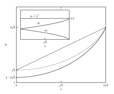
Figure 6.4: The quantity $d_{c}$ (see text) vs. $\lambda$ (that parameterizes the family of Bell operators (6.46)). The long dashed line corresponds to the minimum possible amount of entanglement ($d_{c}^{MM}$). The short dashed curve corresponds to the inference technique here advanced ($d_{c}^{I}$), the solid one to Jaynes’s MaxEnt approach ($d_{c}^{ME}$). The two inference schemes are seen to produce “fake” inferred entanglement. Inset: The eigenvalues of $\rho_{I}$ versus $\lambda$ for $\langle\hat{D}\rangle=d_{c}$. Note that $p_{1}=1/2^{+}\equiv 1/2+\epsilon$.

$$p_{3}\, = \,\{d+\lambda-(2\sqrt{2}+\lambda)p_{1}+(2\sqrt{2}-\lambda)p_{4}\}/2\lambda,$$ (6.48)

$$p_{2}\, = \,\{\lambda-d+(2\sqrt{2}-\lambda)p_{1}-(2\sqrt{2}+\lambda)p_{4}\}/2\lambda.$$ (6.49)

In view of the above facts i) and ii), it is obvious that one minimizes entanglement by letting $p_{4}\rightarrow 0$. Finally, we maximize the von Neumann entropy, which uniquely fixes the weight $p_{1}$, and yields the desired, final state $\hat{\rho}_{I}$. The present treatment can be regarded as a new inference procedure, reminiscent of that of Horodecki’s, although it does not coincide with it. It is introduced to show just how insidious the problem of overestimating the amount of entanglement problem really is.

For each value of $\lambda$ we have, of course, a different Bell observable and confront three (in principle, different) entanglement values, namely, (i) minimum minimorum $E_{MM}$, (ii) the one corresponding to $\hat{\rho}_{ME}$, namely, $E_{ME}$, and, (iii) the one corresponding to $\hat{\rho}_{I}$, that is, $E_{I}$, which will yield three monotonous $\lambda$-curves when these amounts of entanglement are plotted as a function of $d$. Let us call $d_{critical}\equiv d_{c}$ those particular $d$-values for which $E=0$. Fig.6.4 depicts, as a function of $\lambda$, the three values $d_{c}^{MM,\,ME,\,I}$. It is easy to see that $d_{c}^{MM}=\frac{2\sqrt{2}+\lambda}{2}.$ Clearly, at $\lambda=0$ we have $d_{c}^{MM}=d_{c}^{I}$. The three curves coincide at $\lambda=2\sqrt{2}$. At intermediate $\lambda$-values, both $\hat{\rho}_{ME}$ and $\hat{\rho}_{I}$ are afflicted by the problem of overestimation of entanglement. (The inset depicts $p_{1},\,p_{2},\,p_{3}\,\,versus\,\,\lambda$ for $d=d_{c}$, where $p_{1}$ is slightly larger that $1/2$, by an infinitesimal amount $\epsilon$.)

Entanglement boundaries

One would like to know, given some piece of information (constraint), just which state is the one with the minimum possible amount of entanglement. We will study now the whole set of states compatible with one a priori known mean value in a search for this desideratum. We restrict our consideration to operators diagonal in the Bell basis. Let ${\hat{B}}=(B_{1},B_{2},B_{3},B_{4})$ be a general operator describing some system’s observable, and $\hat{\rho}=(p_{1},p_{2},p_{3},p_{4})$ a normalized state with $b=Tr(\hat{\rho}\hat{B})=p_{1}B_{1}+p_{2}B_{2}+p_{3}B_{3}+p_{4}B_{4}$. Although in this Chapter we shall describe only non-degenerate ${\hat{B}}$, the most general case is considered in [185].

For the sake of simplicity we assume the eigenvalues of ${\hat{B}}$ ordered according to $B_{1}<B_{2}<B_{3}<B_{4}$, without loss of generality. Let us regard $p_{1}$ and $p_{2}$ as the“true” unknown weights. Thus, the positivity and normalization of $\hat{\rho}$ clearly determine the remaining weights. One writes then the final state in the following fashion $\hat{\rho}=(p_{1},p_{2},p_{3},p_{4})$, with

$$p_{3}\, = \,\{B_{4}-b+(B_{1}-B_{4})p_{1}+(B_{2}-B_{4})p_{2}/[B_{4}-B_{3}]\},$$ (6.50)

$$p_{4}\, = \,\{b-B_{3}-(B_{1}-B_{4})p_{1}-(B_{2}-B_{4})p_{2}/[B_{4}-B_{3}]\}.$$ (6.51)

Forcing both $p_{1}$ and $p_{2}$ to vanish, the remaining weights $p_{3}$ and $p_{4}$ adopt minimum or maximum values, depending on the value of $b$. This defines for the interval $[B_{3},B_{4}]$ low and high entanglement-degree states. Repeating this procedure for the remaining $\frac{N(N-1)}{2}=6$ different ways of selecting two independent weights (out $N=4$), we obtain a whole family of high and low degree of entanglement states.

To be more precise, these states are described by the following family

$$\hat{\rho}_{\lambda,\kappa}=(\frac{b-\kappa}{\lambda-\kappa},0,\frac{\lambda-b}{\lambda-\kappa},0)$$ (6.52)

where both $\kappa$ and $\lambda$ ($\kappa<\lambda$) belong to the set $\{B_{i}\}$. The positions of the non-zero weights should ensure that the condition $b=Tr(\hat{\rho}_{\lambda,\kappa}\hat{B})$ is fulfilled. We are now in a condition to ascertain which is the minimum amount of entanglement for a given observable $\hat{B}$ or, conversely, which states define the curve of least possible entanglement in the $({\it b},E({\it b}))$-plane. By evaluation of the concurrence [158] of (6.52), it is easy to show that the state $\hat{\rho}_{\lambda=B_{2},\kappa=B_{1}}$ defines the least entangled state for constraints ranging from $b=B_{1}$ up to $b=\frac{B_{1}+B_{2}}{2}$, where the entanglement of formation keeps vanishing till we reach, for our constraint, the value $b=\frac{B_{3}+B_{4}}{2}$. Afterwards, the state $\hat{\rho}_{\lambda=B_{4},\kappa=B_{3}}$ is the one that determines the curve of minimum possible entanglement, until we reach for $b$ the value $b=B_{4}$. These features are illustrated in Fig.6.5 for $\hat{B}=(2,-2,1,-1)$. A reasonable sample of all possible physical states is plotted (randomly) as background. The above determined boundaries are also drawn (dashed lines), together with the amounts of entanglement corresponding to both ${\hat{\rho}_{ME}}$ (dot-dashed line) and ${\hat{\rho}_{E}}$ (solid line).

Figure 6.5: States $\hat{\rho}_{\lambda,\kappa}$ defining the entanglement boundaries are plotted (dashed lines), together with the back-ground of accessible states. See text for details and Ref. [185].

6.3 Concluding remarks

In this Chapter we have exhaustively investigated Horodecki’s “fake” inferred entanglement problem, related with the use of the maximum entropy principle, with reference to distinct inference schemes, and advanced a new one, reminiscent of Horodecki’s, for dealing with more general observables than the Bell-CHSH one (6.1).

There is no doubt that Jaynes’ MaxEnt principle has to play an important role in any appropriate scheme for the inference of entangled quantum states. Indeed, one of the most remarkable features of Jaynes’ principle is its robustness: usually, when it seems to fail, the real problem is not the inadequacy of the MaxEnt principle itself, but rather that some piece of relevant (prior) information is not being taken into account. In point of fact it was pointed out in [182] that the various inference schemes advanced to solve the fake inferred entanglement problem admit of an interpretation within the strictures of Jaynes’ approach. These inference prescriptions may be regarded as implementations of the MaxEnt principle in which some extra prior information (that may not consists just of the expectation values of some observables) is assumed to be known. This is certainly the case with Rajagopal’s MaxEnt minimum-$\sigma^{2}$ proposal, which assumes extra information related to the square of the relevant observable. However, the results reported here show that this approach works only in very special situations.

Besides enabling us to asses the usefulness of the minimum-$\sigma^{2}$ scheme, we shed some light on the entanglement features exhibited by the standard MaxEnt principle within contexts more general than those previously considered in the literature [176, 178, 179, 180].

Summing up, we conclude that:

• For arbitrary operators of the type (6.17), Rajagopal’s $\sigma^{2}$-scheme does not provide a satisfactory solution as in the Bell-CHSH case.

• For a quite general Bell diagonal observable ${\hat{B}}=(B_{1},B_{2},B_{3},B_{4})$, we have studied all the normalized states $\hat{\rho}$ (pure and mixed) such that $Tr[\hat{\rho}\hat{B}]=b$ and established just which is the one with minimum (maximum) amount of entanglement. We have drawn the “entanglement boundaries” in the $(b,E(b))$-plane. Once these states have been found, the problem of “fake” inferred entanglement is immediately solved.

Chapter 7 Detection of entanglement at work: hierarchy of separability criteria. Volume occupied by the set of unentangled states according to different criteria

The development of criteria for entanglement and separability is one aspect of the current research efforts in quantum information theory that is receiving, and certainly deserves, considerable attention [118], and so we devote the present Chapter to its study. Indeed, much progress has recently been made in consolidating such a cornerstone of the theory of quantum entanglement [118]. The relevant state-space here is of a high dimensionality, already 15 dimensions in the simplest instance of two-qubit systems. The systematic exploration of these spaces can provide us with valuable insight into some of the theoretical questions extant.

As a matter of fact, important steps have been recently made towards a systematic exploration of the space of arbitrary (pure or mixed) states of composite quantum systems [186, 187, 188] in order to determine the typical features exhibited by these states with regards to the phenomenon of quantum entanglement [186, 187, 188, 189, 190, 191, 192].

It is well known that, for a composite quantum system, a state described by the density matrix $\rho$ is called “entangled” if it can not be represented as a mixture of factorizable pure states. Otherwise, the state is called separable. The separability question has interesting echoes in information theory and its associate information measures or entropies, as adressed in Chapter 4. We know that the early motivation for the studies reported in [127, 128, 129, 130, 131, 132, 133, 134] was the development of practical separability criteria for density matrices. However, the discovery by Peres of the partial transpose criteria, which for two-qubits and qubit-qutrit systems turned out to be both necessary and sufficient, rendered that original motivation somewhat outmoded. A crucial fact, it is not possible to find a necessary and sufficient criterion for separability based solely upon the eigenvalue spectra of the three density matrices $\rho_{AB},\rho_{A}=Tr_{B}[\rho_{AB}]$, and $\rho_{B}=Tr_{A}[\rho_{AB}]$ associated with a composite system $A\oplus B$ [126].

Interesting concepts that revolve around the separability issue have been developed over the years. A comprehensive account is given in Terhal in [118]. Among them we find criteria like the so-called Majorization, Reduction and Positive Partial Transpose (PPT) (all of them described in Chapter 4), together with the concept of distillability. Certainly, quantum entanglement is a fundamental aspect of quantum physics that deserves to be investigated in full detail from all possible points of view. The chain of implications,

${\it\rho\,\,separable\rightarrow PPT\rightarrow reduction\rightarrow majorization\rightarrow q-entropic}$

and the related inclusion relation, among the different separability criteria is certainly a vantage point worth of detailed scrutiny [139].

It is our purpose here to revisit, with such a goal in mind, the separability question by means of an exhaustive Monte Carlo exploration involving the whole space of pure and mixed states. Such an effort should shed some light on the inclusion issues that interest us here. Concrete numerical evidence will thus be provided on the relations among the separability criteria. We will then be able to quantify, for a bipartite system of arbitrary dimension, the proportion (or volume) of states $\rho$ that can be distilled according to a definite criterion.

Although the complete description of the separability criteria was already given in Chapter 4, let us briefly sketch the mathematics of these criteria. From a historic viewpoint, the first separability criterion is that of Bell (see Chapter 1 in the Introduction). For every pure entangled state there is a Bell inequality that is violated. It is not known, however, whether in the case of many entangled mixed states, violations exist. There does exist a witness for every entangled state though [193]. It was shown by Horodecki et al. that a density matrix $\rho\equiv\rho_{AB}$ is entangled if and only if there exists an entanglement witness (a hermitian superoperator $\hat{W}=\hat{W}^{\dagger}$) such that

$$Tr\,\hat{W}\,\rho \leq 0,\,\,\,\,{\rm while}$$

$$Tr\,\hat{W}\,\rho_{s} \geq 0,\,\,{\rm for\,\,all\,\,separable\,\,states\,\,\rho_{s}}.$$ (7.1)

Also, an important LOCC operational separability criterion, necessary but not sufficient, is provided by the positive partial transpose (PPT) one. Let $T$ stand for matrix transposition. The PPT requires that

$$[\hat{1}\otimes\hat{T}](\rho)\geq 0.$$ (7.2)

Another operational criterion is reduction, that is satisfied, for a given state $\rho\equiv\rho_{AB}$, when both [118]

$$\hat{1}\otimes\rho_{B}-\rho \geq 0$$

$$\rho_{A}\otimes\hat{1}-\rho \geq 0.$$ (7.3)

As we know, the distillable entanglement is the maximum asymptotic yield of singleton states that can be obtained, via LOCC, from a given mixed state. It was shown in [120] that any entangled mixed state of two qubits can be distilled to obtain the singleton. However, there are entangled mixed states (in higher dimensions) that cannot be distilled, so that they are useless for quantum communication. In our scenario an important fact is that all states that violate the reduction criterion are distillable [121].

Majorization criterion compares the spectra of two matrices in a special way. Let $\{\lambda_{i}\}$ be the set of eigenvalues of the matrix $\xi_{1}$ and $\{\gamma_{i}\}$ be the set of eigenvalues of the matrix $\xi_{2}$. We assert that the ordered set of eigenvalues $\vec{\lambda}$ of $\xi_{1}$ majorizes the ordered set of eigenvalues $\vec{\gamma}$ of $\xi_{2}$ (and writes $\vec{\lambda}\succ\vec{\gamma}$) when $\sum_{i=1}^{k}\,\lambda_{i}\,\geq\,\sum_{i=1}^{k}\,\gamma_{i}$ for all $k$. It has been shown [126] that, for all separable states $\rho_{AB}\equiv\rho$,

$$\vec{\lambda}_{\rho_{A}} \succ \vec{\lambda}_{\rho},\,\,{\rm and}$$

$$\vec{\lambda}_{\rho_{B}} \succ \vec{\lambda}_{\rho}.$$ (7.4)

There is an intimate relation between this majorization criterion and entropic inequalities, as discussed in [118, 127].

We ommit the description of the entropic criteria [194], which will constitute the subject of main study in the next Chapter.

7.1 Separability probabilities: exploring the whole state space

We shall perform a systematic numerical survey of the properties of arbitrary (pure and mixed) states of a given quantum system by recourse to an exhaustive exploration of the concomitant state-space ${\cal S}$. To such an end it is necessary to introduce an appropriate measure $\mu$ on this space. Such a measure is needed to compute volumes within ${\cal S}$, as well as to determine what is to be understood by a uniform distribution of states on ${\cal S}$. The natural measure that we are going to adopt here is taken from the work of Zyczkowski et al. [186, 187]. An arbitrary (pure or mixed) state $\rho$ of a quantum system described by an $N$-dimensional Hilbert space can always be expressed as the product of three matrices,

$$\rho\,=\,UD[\{\lambda_{i}\}]U^{\dagger}.$$ (7.5)

Here $U$ is an $N\times N$ unitary matrix and $D[\{\lambda_{i}\}]$ is an $N\times N$ diagonal matrix whose diagonal elements are $\{\lambda_{1},\ldots,\lambda_{N}\}$, with $0\leq\lambda_{i}\leq 1$, and $\sum_{i}\lambda_{i}=1$. The group of unitary matrices $U(N)$ is endowed with a unique, uniform measure: the Haar measure $\nu$ [195]. On the other hand, the $N$-simplex $\Delta$, consisting of all the real $N$-uples $\{\lambda_{1},\ldots,\lambda_{N}\}$ appearing in (7.5), is a subset of a $(N-1)$-dimensional hyperplane of ${\cal R}^{N}$. Consequently, the standard normalized Lebesgue measure ${\cal L}_{N-1}$ on ${\cal R}^{N-1}$ provides a natural measure for $\Delta$. The aforementioned measures on $U(N)$ and $\Delta$ lead then to a natural measure $\mu$ on the set ${\cal S}$ of all the states of our quantum system [186, 187, 195], namely,

$$\mu=\nu\times{\cal L}_{N-1}.$$ (7.6)

All our present considerations are based on the assumption that the uniform distribution of states of a quantum system is the one determined by the measure (7.6). Thus, in our numerical computations we are going to randomly generate states according to the measure (7.6). In the forthcoming Chapters we will be dealing several times with this measure, which is fully described in Appendix B.

7.2 Survey’s results

The overall scenario

An overall picture of the situation we encounter is sketched in Fig.7.1. The set of all mixed states presents an onion-like shape, as conjectured by Terhal [118]. Which among these states are separable? As reviewed above, several criteria are available. We start with the $q$-entropic one. By using a definite value of $q$, namely $q=\infty$, and the sign of the associated, conditional $q$-entropy, we are able to define a closed sub-region, whose states are supposedly separable. This region has a definite border, that separates it from the sub-region of states entangled according to this criterion. What we see now is that, if we use now other separability-criteria, the associated sub-regions shrink in a manner prescribed by the particular criterion one employs. The shrinking process ends when one reaches the sub-region defined by the Positive Partial Transpose (PPT) criterion, which is a necessary and sufficient separability condition for $2\times 2$ and $2\times 3$ systems, being only necessary for higher dimensions.

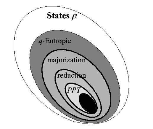
Figure 7.1: Schematics of the inclusion relations among separability criteria as given by the volume occupied by states $\rho$ for a given dimension $N$ which fulfil them.

Summing up, the volume of states which are separable according to different criteria diminish as we use stronger and stronger criteria. There is a first shrinking stage associated to entropic criteria, from its Von Neumann ($q=1$) size, as $q$ grows, to the limit case $q\rightarrow\infty$ [194]. A second stage involves majorization, reduction, and, finally positive partial transpose (PPT) [118].

PPT and Reduction

We report now on our state-space exploration with regards to the probability of finding a state with positive partial transpose. The results are depicted in Fig.7.2. The solid line corresponds to states with dimension $N=2\times N_{2}$, while the dashed line corresponds to $N=3\times N_{2}$ states. Note how similar are the pertinent values in both cases. The tiny difference between them can be inspected in the inset (a semi-logarithmic plot). To a good approximation, our PPT probabilities decrease exponentially. There exist lower bounds to the volume of separable states. In [161], G. Vidal and R. Tarrach show that the probability of finding a separable state in a $n$-party system with $N$-dimensional Hilbert space is

$$P_{sep}\,\geq\,\bigg{(}\frac{1}{1\,+\,\frac{N}{2}}\bigg{)}^{(n-1)(N-1)}$$ (7.7)

which is clearly nonzero for finite systems.

Figure 7.2: Probability of finding a state with positive partial transpose. The solid line corresponds to states with dimension $N=2\times N_{2}$, while the dashed line corresponds to $N=3\times N_{2}$ states. The difference between these curves can be appreciated in the inset (semi-logarithmic plot). Our probabilities decrease, to a good approximation, in exponential fashion.

Figure 7.3: Probability of finding a state fulfilling the reduction criterion for $N=2\times N_{2}$ (solid line) and $N=3\times N_{2}$ (dashed line). PPT and reduction coincide for $N=2\times N_{2}$ systems.

Fig.7.3 deals instead with the probability of finding a state which obeys the strictures of the reduction criterion, for $N=2\times N_{2}$ (solid line) and $N=3\times N_{2}$ (dashed line). As a matter of fact, PPT and reduction coincide for $N=2\times N_{2}$. It is known that if a state satisfies PPT, it automatically verifies the reduction criterion [118]. We have demonstrated that, at least in the $N=2\times N_{2}$-instance, the converse is also true [139]. However, in the $N=3\times N_{2}$-case, it is much more likely to encounter a state that verifies reduction than one that verifies PPT.

Entropic criteria and Majorization

We begin with a brief recapitulation of former $q$-entropic results. The situation encountered in [196] was that the “best” result within the framework of the “classical $q$-entropic inequalities” as a separability criterion was reached using the limit case $q\rightarrow\infty$, but considerably less attention was paid to other values of $q$. This was remedied in [194], where the question of $q$-entropic inequalities for finite $q$-values was extensively discussed. It was there re-confirmed that the above mentioned limit case does indeed the better job as far as separability questions are concerned [194]. For such a reason, this limit $q$-value is the only one to be employed below.

Figure 7.4: Probability of finding a state whose two relative $q$-entropies are positive for $q\rightarrow\infty$ (dashed curves). The probability that a state be completely majorized by both of their subsystems is represented by the solid line. Bottom: curves correspond to states $\rho$ with $N=2\times N_{2}$. Top: $N=3\times N_{2}$.

In Fig.7.4 we depict the probability of finding a state which, for $q\rightarrow\infty$, has its two conditional $q$-entropies positive (dashed curves). In view of the intimate relation of entropic inequalities with majorization [118, 127], we also analyze in Fig.7.4 the probability that a state is completely majorized by both of their subsystems (solid line). It is shown in [127] that, if $\rho_{AB}$ satisfies the reduction criterion, its two associated conditional $q$- entropies are non-negative as well.

In the same work the authors assert that majorization is not implied by the conditional entropy criteria. Our results confirm this assessment. In Fig.7.4, the lower curves correspond to states $\rho$ with $N=2\times N_{2}$, while the upper curves have $N=3\times N_{2}$. Majorization results and $q$-entropic do coincide for two-qubits systems ($N_{1}=N_{2}=2$). More generally, majorization probabilities are a lower bound to probabilities for conditional $q$-entropic positivity, an interesting new result, as far as we know. Notice also that the two approaches yield quite similar results in the $N=3\times N_{2}$ case.

Comparing more than two criteria together

We compare now the reduction criterion to the PPT one. The former is implied by the latter but is nonetheless a significant condition since its violation implies the possibility of recovering entanglement by distillation, which is as yet unclear for states that violate PPT [127]. Fig.7.5 a) depicts the probability that state $\rho$ with $N=3\times N_{2}$ either:

1. has a positive partial transpose and does not violate the reduction criterion, or

2. has a non positive partial transpose and violates reduction.

Remember that in the case $N=2\times N_{2}$, the two criteria always coincide [118]. For $3\times N_{2}$ the agreement between the two criteria becomes better and better as $N_{2}$ augments.

Figure 7.5: a) Probability that the state $\rho$ with $N=3\times N_{2}$ either has i) a positive partial transpose and does not violate the reduction criterion, or ii) has a non positive partial transpose and violates reduction. In the case $N=2\times N_{2}$ the outcome is always unity. b) Probability that i) PPT and majorization (solid line) and, ii) PPT and the $q$-entropic criterion (dashed line) lead to the same conclusion regarding separability. Top: $N=2\times N_{2}$. Bottom: $N=3\times N_{2}$.

Of more interest is to compare the relations among PPT, majorization, and the entropic criteria (Fig.7.5b), since it is not yet known how the majorization criterion is related to other separability criteria like PPT, undistillability, and reduction [127]. In this vein, Fig.7.5 b) plots the “coincidence-probability” between, respectively,

1. PPT and majorization (solid line), and

2. PPT and the $q$-entropic criterion (dashed line).

The curves on the top correspond to $N=2\times N_{2}$, while those at the bottom to $N=3\times N_{2}$. In this last case the two curves agree with each other quite well.

The conclusion here is that, as $N_{2}$ augments, the probability of coincidence among the three criteria, and in particular between majorization and PPT (our main concern), rapidly diminishes at first, and stabilizes itself afterwards. For two qubits the three criteria do agree with each other to a large extent.

Fig.7.6 a) depicts the probability that, for a given state $\rho$,

1. reduction and majorization (solid line) and

2. reduction and the $q$-entropic criterion (dashed line)

yield the same conclusion as regards separability. Without PPT in the game, and opposite to what we encountered in Fig.7.5, we find better coincidence for $N=3\times N_{2}$ systems (top) than for $N=2\times N_{2}$ (bottom). The deterioration of the degree of agreement as $N_{2}$ grows is similar to that of Fig.7.5, though.

Figure 7.6: a) Probability that reduction and majorization (solid line) and reduction and the $q$-entropic criterion (dashed line) yield the same conclusion reagrding separability. Top: $N=3\times N_{2}$. Bottom: $N=2\times N_{2}$ (lower curves). b) Probability that a state, for $q\rightarrow\infty$, either i) has both positive relative $q$-entropies and fulfils majorization, or ii) has a negative relative $q$-entropy and is majorized by both of their subsystems. The solid line corresponds to the case $N=2\times N_{2}$, while the dashed line corresponds to $N=3\times N_{2}$.

Fig.7.6b) represents the probability that a state, for $q\rightarrow\infty$, either:

1. has both positive conditional $q$-entropies and satisfies the majorization criterion, or

2. has a negative conditional $q$-entropy and is majorized by both of their subsystems.

The solid line corresponds to the case $N=2\times N_{2}$, while the dashed lines corresponds to the $N=3\times N_{2}$ instance. These results together with those of Figs.7.4-7.5 could be read as implying that majorization and the $q$-entropic criteria provide almost the same answer for dimensions greater or equal than $N=3\times N_{2}$.

Figure 7.7: Total probability that all criteria considered in the present work lead to the same conclusion regarding separability. Probabilities are plotted as a function of the total dimension $N=N_{1}\times N_{2}$, with $N_{1}=2$ (solid line) and $N_{1}=3$ (dashed line).

Finally, in Fig.7.7 we look for the probability $P_{agree}$ that all criteria considered in the present work do lead to the same conclusion on the separability issue. $P_{agree}$ is plotted as a function of the total dimension $N=N_{1}\times N_{2}$, with $N_{1}=2$ (solid line) and $N_{1}=3$ (dashed line). The agreement is quite good for two qubits, deteriorates first as $N_{2}$ grows, and rapidly stabilizes itself around a value of 0.26 for $N_{1}=2$ and of 0.1 for $N_{1}=3$.

Distilling

Let us at now consider the results plotted in Fig.7.8. We ask first for the relative number of states that violate the reduction criterion and are thus distillable [120] (solid line), and appreciate the fact that, as $N$ grows, so does the probability of finding distillable states. On the other hand, the probability of encountering states that violate the majorization criterion, represented by dashed lines, is much lower than that associated to distillation.

Figure 7.8: Solid line: probability that a state violates the reduction criterion. Dashed line: the same for violation of the majorization criterion. Top: $N=2\times N_{2}$. Bottom: $N=3\times N_{2}$. The dashed curve with crosses represents the case $N=2\times N_{2}$, while the one with squares indicates the $N=3\times N_{2}$ instance.

For both criteria, the upper solid line corresponds to the case $N=2\times N_{2}$, and the lower one to $N=3\times N_{2}$. The dashed curve with crosses represents the case $N=2\times N_{2}$, while the one with squares indicates the $N=3\times N_{2}$ instance. The dependence with $N_{2}$ of the dashed curves (majorization violation) is not so strong as that of the solid ones (distillability). Our results are lower bounds to the total volume of states that can be distilled.

7.3 Concluding remarks

In this Chapter, we have explored the application of different separability criteria by recourse to an exhaustive Monte Carlo exploration involving the pertinent state-space of pure and mixed states. The corresponding chain of implications of different criteria is in such a way numerically elucidated. We have also quantified, for a bipartite system of arbitrary dimension, the proportion of states $\rho$ that can be distilled according to a definite criterion.

To be more precise, we have performed a systematic numerical survey of the space of pure and mixed states of bipartite systems of dimension $2\times N_{2}$ and $3\times N_{2}$ in order to investigate the relationships ensuing among different separability criteria. Our main results are

• Regarding the line of separability implication, our graph in Fig.7.1 constitutes a confirmation of some propositions in Terhal’s work [118]

• It is known that if a state satisfies PPT, it automatically verifies the reduction criterion [118]. In the present work we show that in the $N=2\times N_{2}$-instance, the converse is also true. In the $N=3\times N_{2}$-case, it is much more likely to encounter a state that verifies reduction than one that verifies PPT.

• We have numerically verified the assertion made in [127] that majorization is not implied by the conditional entropic criteria. Majorization results and $q$-entropic criteria coincide for two-qubits systems. In general, majorization probabilities constitutes lower bounds for conditional $q$-entropic positivity.

• Regarding the relation between majorization and PPT, the agreement between the criteria deteriorates as $N_{2}$ grows.

• For dimensions $\geq 3\times N_{2}$, as illustrated by Figs.7.4-7.5, majorization and the $q$-entropic criteria provide almost the same answers.

• Lower bounds to the total volume of states that can be distilled are found.

We believe that the results of this numerical exploration shed some light on the intricacies of the separability issue. Indeed, the size of the volume of separable states would reflect the fact important for numerical analysis of entanglement, to what extent the separable or entangled states are typical. But, according to [140], also there appeared a technical motivation: the considerations on volume of separable states lead of important results concerning the question of relevance of entanglement in quantum computing [197], specifically NMR quantum computing. These considerations proved to be crucial for analysis of the experimental implementation of quantum algorithms in high-$T$ systems via NMR methods. This is because a generic state used in this approach is the maximally mixed one with a small admixture of some pure entangled state. In [197] the sufficient conditions of the above sort were further developed and it was concluded, that in all the NMR quantum computing experiments performed to date the admixture of the pure state was too small. Thus the total state used in these experiments was separable.

Chapter 8 Conditional $q$-entropies and quantum separability

Some entangled states of quantum composite systems (in particular, all pure entangled states) exhibit the notable property of having an entropy smaller than the entropies of their subsystems. This feature of composite quantum systems, and its connections with other of their entanglement-related properties, has been recently investigated by several authors [118, 127, 128, 129, 130, 131, 132, 133, 134, 198, 199]. The phenomenon of entanglement is one of the most fundamental and non-classical features exhibited by quantum systems [2, 110]. Quantum entanglement is the basic resource required to implement several of the most important processes studied by quantum information theory [12, 34, 110, 114, 115, 140], such as quantum teleportation [102], superdense coding [99] and the exciting issue of quantum computation [34]. Due to the significance of quantum entanglement, it is important to survey the state space of composite quantum systems, in order to get a clear picture of the concomitant entanglement properties, and of the relationships between entanglement and other relevant features exhibited by the quantum states. Significant advances have been made by a program that attempts performing a systematic exploration of the space of arbitrary (pure or mixed) states of composite quantum systems [186, 187, 188] in order to determine the characteristic features shown by these states with regards to the phenomenon of quantum entanglement [186, 187, 188, 189, 190, 191, 192, 194].

Separable quantum states share with classical composite systems the following basic property: the entropy of any of its subsystems is always equal or smaller than the entropy characterizing the whole system [126]. In contrast, as already mentioned, a subsystem of a quantum system described by an entangled state may have an entropy greater than the entropy of the whole system, thus violating the concomitant classical entropic inequalities. This situation holds for the well known von Neumann entropy, as well as for the more general $q$-entropic (or $q$-information) measures [118, 127, 128, 129, 130, 131, 132, 133, 134, 198, 199], which incorporate both Rényi’s [135] and Tsallis’ [136, 137, 138] families of measures as special instances. These entropic functionals are characterized by a real parameter $q$.

The alluded to classical entropic inequalities constitute necessary and sufficient separability criteria for pure states. The situation is, however, more involved in the case of mixed states. In the latter case we can find entangled states that do not violate these inequalities. Consequently, the classical entropic inequalities provide only necessary separability criteria. As a matter of fact, the main motivation for studying the classical entropic inequalities (and their violation by some entangled states) is not any more the development of practical separability criteria. This is the case particularly since the introduction of the Positive Partial Transposition (PPT) criterion by Peres [123], and the related results obtained by the Horodecki s [193]. However, the violation of the classical entropic inequalities is interesting in its own right, because they constitute, from the perspective of classical physics, a highly counterintuitive property exhibited by some entangled quantum states. Moreover, this non-classical feature of certain entangled states is of a clear and direct information-theoretical nature.

The goal of the present Chapter is to investigate further aspects of the relationship between quantum separability and the violation of the classical $q$-entropic inequalities.

8.1 Features of conditional $q-$entropies of composite quantum systems

By performing a systematic numerical survey of the space of pure and mixed states of bipartite systems of any dimension we are about to determine, for different values of the entropic parameter $q$, the volume in state space occupied by those states characterized by positive values of the conditional $q$-entropies. We pay particular attention to the monotonic tendency shown by these separability ratios as they evolve with $q$ from finite values to the limiting case $q\rightarrow\infty$, for any Hilbert space’s dimension.

8.1.1 $q$-Conditional entropies

As we have shown in Chapter 4, the “$q$-entropies” depend upon the eigenvalues $p_{i}$ of the density matrix $\rho$ of a quantum system through the quantity $\omega_{q}=\sum_{i}p_{i}^{q}$. More explicitly, we shall consider either the Rényi entropies [135],

$$S^{(R)}_{q}\,=\,\frac{1}{1-q}\,\ln\left(\omega_{q}\right),$$ (8.1)

or the Tsallis’ entropies [136, 137, 138]

$$S^{(T)}_{q}\,=\,\frac{1}{q-1}\bigl{(}1-\omega_{q}\bigr{)},$$ (8.2)

which have found many applications in many different fields of Physics. In the $q=2-$case, $S_{q=2}$ is often called the linear entropy $\mathcal{S}_{L}$ [189]. These entropic measures incorporate the important (because of its relationship with the standard thermodynamic entropy) instance of the von Neumann measure, as a particular limit ($q\rightarrow 1$) situation

$$S_{1}\,=\,-\,Tr\left(\hat{\rho}\ln\hat{\rho}\right).$$ (8.3)

Tsallis’ and Rényi’s measures are related through $S^{(T)}_{q}\,=\,F(S^{(R)}_{q}),$ where the function $F$ is given by $F(x)=\left\{e^{(1-q)x}-1\right\}/(1-q).$ As an immediate consequence, for all non vanishing values of $q$, Tsallis’ measure $S^{(T)}_{q}$ is a monotonic increasing function of Rényi’s measure $S^{(R)}_{q}$. We will be here rather more interested in ${\it conditional\,q-entropies}$ than in total entropies, because of the former’s relation with the issue of quantum separability. Conditional entropic measures are defined as

$$S^{(T)}_{q}(A|B)\,=\,\frac{S^{(T)}_{q}(\rho_{AB})-S^{(T)}_{q}(\rho_{B})}{1+(1-q)S^{(T)}_{q}(\rho_{B})}$$ (8.4)

for the Tsallis case, while its Rényi counterpart is

$$S^{(R)}_{q}(A|B)\,=\,S^{(R)}_{q}(\rho_{AB})-S^{(R)}_{q}(\rho_{B}).$$ (8.5)

Notice that the denominator in (8.4), $1+(1-q)S_{q}\,=\,w_{q}\,>\,0$ is always positive. Consequently, as far as the sign of the conditional entropy is concerned, the denominator in (8.4) can be ignored. Now, since Tsallis’ entropy is a monotonous increasing function of Rényi’s, it is plain that (8.4) has always the same sign as (8.5). The matrix $\rho_{AB}$ denotes an arbitrary quantum state of the composite system $A\otimes B$, not necessarily factorizable nor separable, and $\rho_{B}=Tr_{A}(\rho_{AB})$ (the conditional $q$-entropy $S^{(T)}_{q}(B|A)$ is defined in a similar way as (8.4), replacing $\rho_{B}$ by $\rho_{A}=Tr_{B}(\rho_{AB})$). Interest in the conditional $q$-entropy (8.4) arises in view of its relevance with regards to the separability of density matrices describing composite quantum systems [132, 133]. For separable states, we have [127]

$$S^{(T)}_{q}(A|B) \geq 0,$$ (8.6)

$$S^{(T)}_{q}(B|A) \geq 0.$$ (8.7)

As already mentioned, there are entangled states (for instance, all entangled pure states) characterized by negative conditional $q$-entropies. That is, for some entangled states one (or both) of the inequalities (8.6) are not verified. Since just the sign of the conditional entropy is important here, we can either use Tsallis’ or Rényi’s entropy, for (8.4) and (8.5) will always share the same sign. In what follows, when we speak of the positivity of either Tsallis’ conditional entropy (8.4) or of Rényi’s conditional entropy (8.5), we will make reference to the “classical $q$-entropic inequalities” issue.

8.1.2 Volumes in state space sccupied by states of special entropic properties.

The systematic numerical study of pure and mixed states of a bipartite quantum system of arbitrary dimension $N=N_{1}\times N_{2}$ requires the introduction of an appropriate measure $\mu$ defined over the corresponding space ${\cal S}$ of general quantum states. Such a measure is necessary in order to compute volumes within the space ${\cal S}$. The measure we are going to adopt in the present approach ($\mu=\nu\times{\cal L}_{N-1}$) was introduced by Zyczkowski et al. in several valuable contributions [186, 187], and is the same employed in Chapter 7 and throughout the present one. All our present considerations are based on the assumption that the uniform distribution of states of a quantum system is the one determined by measure $\mu$ (7.6). Thus, in our numerical computations we are going to randomly generate states according to measure (7.6). The situation that we shall encounter in next section is the following one: the volume in phase space corresponding to those states complying with the classical $q$-entropic inequalities monotonically decreases as the entropic parameter $q$ increases, adopting its minimum value in the limit case $q\rightarrow\infty$. In this limit case, the volume of states with positive conditional entropies adopts simultaneously: i) its lowest value and also ii) the one most closely resembling that of the set of states with positive partial transpose (PPT). The volume of states with positive conditional $q$-entropies is, however, even in the limit case $q\rightarrow\infty$, larger than the volume associated with states with a positive partial transpose. This means that, regarded as a separability criterion, the classical entropic inequality with $q=\infty$ is (among the conditional $q$-entropic criteria) the strongest one, though it is not as strong as the PPT criterion (see Fig.7.1). In point of fact, it has been proven that there is no necessary and sufficient criteria for quantum separability based solely on the eigenvalues of $\rho_{AB}$, $\rho_{A}$, and $\rho_{B}$. Our main concern here is not the study of the classical inequalities qua separability criteria. Their study is interesting per se because it provides us with additional insight into the issue of quantum separability, on account of their intuitive information-theoretical nature. We want to survey the state-space in order to obtain a picture, as detailed as possible, of i) how the signs of the $q$-conditional entropies are correlated with other entanglement-related features of quantum states, and ii) how these correlations depend both on the value of $q$ and on the dimensionality of the systems under consideration.

As reported in [196], the volume occupied by states with positive values of the conditional $q$-entropies decreases with $q$ in a monotonous fashion as the entropic parameter grows from finite $q$-values to $q=\infty$. It is to be remarked that some authors had previously conjectured [132] that the conditional $q$-entropy $S_{q}(A|B)[\rho]$, evaluated in each particular density matrix $\rho$, is a monotonous decreasing function of $q$. This conjecture implies that it should be enough to consider the value $q\rightarrow\infty$ in order to decide on the positivity of the conditional $q$-entropies for all $q$. If this conjecture were true it would lead, as an immediate consequence, to the monotonous behaviour (as a function of $q$) of the volume of states with positive values of the conditional $q$-entropies.

Alas, one can find several low-rank counterexamples to the monotonicity of the conditional Tsallis or Rényi entropies with $q$ (a particularly interesting case of non-monotonicity with $q$ of Tsallis’ conditional entropies has been recently discussed by Tsallis, Prato, and Anteneodo in [199]). A rather surprising situation ensues: the volumes associated with positive valued conditional $q$-entropies behave in a monotonous way in spite of the fact that the alluded to conjecture is not valid. One of the aims of the present effort is precisely to investigate this point in more detail. By recourse to a Monte Carlo calculation we have determined numerically (both for two-qubits and qubit-qutrit systems) the proportion of states which behave monotonously as $q$ changes. This involves exploring either the $15$-dimensional space of two-qubits ($N=4$) or the $35$-dimensional space of one qubit-one qutrit mixed states. Table 8.1 shows the results for different ranks, dimensions, and entropies used for the mixed state $\rho$. In each case (that is, for each set of values for $q$, total Hilbert Space dimension $N=N_{1}\times N_{2}$, and rank of $\rho$) we have randomly generated $10^{7}$ density matrices. This implies that the relative numerical error associated with the values reported in Table 8.1 is less than $10^{-3}$. We consider it remarkable that most of the states have a conditional entropy that behaves monotonically with $q$, this fact being more pronounced for the case of the Tsallis entropy. The proportion of these states diminishes as the rank of the state $\rho$ decreases, regardless of the dimension and the conditional entropy used. The general trend suggested by Table 8.1 is that the percentage of states with monotonous conditional $q$-entropies increases with the total (Hilbert space’s) dimension of the system and, for a given total dimension, increases with the rank of the density operator. This is fully consistent with the monotonic behaviour (as a function of $q$) exhibited by the total volume corresponding to states with positive conditional $q$-entropies.

	Tsallis	Rényi
$2\times 2.Rank,\ 4$	0.972	0.719
$Rank,\ 3$	0.850	0.434
$Rank,\ 2$	0.204	0.003
$2\times 3.Rank,\ 6$	0.996	0.888
$Rank,\ 5$	0.99	0.79
$Rank,\ 4$	0.96	0.64
$Rank,\ 3$	0.84	0.38
$Rank,\ 2$	0.32	0.003

Table 8.1: Proportion of states which behave monotonously as $q$ changes. Both Tsallis’ and Rényi’s conditional entropies, for two-qubits and one qubit-one qutrit systems, are considered. For a given dimensionality one is to notice how the system evolves with the rank of the pertinent state $\rho$.

Examples of non-monotonous behaviour of the conditional $q$-entropy are depicted in Fig.8.1, for a pair of two-qubits states of range four. The dashed line corresponds to a state whose conditional entropy, although non-monotonous, remains always positive. The continuous line refers to an entangled state such that $S^{(T)}_{q}(A|B)<0$ for large enough $q$-values. The $q$-interval in which the monotonicity of the last state is broken is depicted in the inset. One gathers form these results that it seems correct to regard $q\rightarrow\infty$ as the right value to ascertain positivity for a single given state $\rho$, as was recently suggested by Abe [134] on the basis of his analysis of a mono-parametric family of mixed states for multi-qudit systems.

Figure 8.1: Conditional Tsallis entropy $S_{q}(B|A)$ for two sample states $\rho$ of a two-qubits system (with rank 4) which do not change in monotonous fashion when $q$ grows. The dashed line corresponds to a state whose conditional entropy remains positive for all $q$-values. The solid line corresponds to a state whose conditional entropy eventually becomes negative (and, consequently, the state becomes entangled) for large values of $q$. The inset depicts, for the last case, details of the rather tiny region where monotonicity is broken. All quantities depicted are dimensionless.

To further explore the issue of monotonicity we have computed the fraction of the total state space volume occupied by (that is, the probabilities of finding) states with positive conditional $q$-entropies (for both (i) different finite values of $q$ and (ii) $q=\infty$), in the case of bipartite quantum systems described by Hilbert spaces of increasing dimensionality [194]. Let i) $N_{1}$ and $N_{2}$ stand for the dimension of the Hilbert space associated with each subsystem, and ii) $N=N_{1}\times N_{2}$ be the dimension of the Hilbert space associated with the concomitant composite system. We have considered two sets of systems: (1) systems with $N_{1}=2$ and increasing values of $N_{2}$, and (2) systems with $N_{1}=3$ and increasing dimensionality. The computed probabilities for the first set of systems are depicted in Fig.8.2, as a function of the total dimension $N$. The case of the second set is depicted in Fig.8.3. In order to obtain each point in Figs. 8.2 and 8.3 (as well as to obtain each of the points appearing in the subsequent Figures in this section) we have randomly generated $10^{7}$ density matrices. This leads to Monte Carlo results with a relative, numerical error less than $10^{-3}$. In Fig.8.2 one plots different values of the probabilities associated with positive conditional $q$-entropy for (a) $q=2,4,8,16,$ and $\infty$ and (b) different values of the total dimension $N$ of the system.

Figure 8.2: Probability of finding a state $\rho$ for systems in $2\times N_{2}$ dimensions which, for different values of $q$, has its two conditional $q$-entropies positive. Different curves are assigned to various values of $q$. These curves “saturate” when the limit $q\rightarrow\infty$ is reached. Also, two regimes of growth with the dimension are to be noticed. See text for details. The inset depicts the concomitant probabilities for PPT. The lines are just a guide for the eye. All quantities depicted are dimensionless.

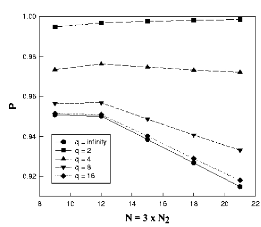
Figure 8.3: Same as in Fig.8.2 for systems of $3\times N_{2}$ dimensions. Values of probabilities are higher and the rate of saturation is different. All quantities depicted are dimensionless.

With respect to the behaviour of these probabilities, one is to focus attention upon two aspects: i) evolution with $q$ for a given $N$ and ii) evolution with the dimension for fixed $q$. In the first instance one clearly sees a common behaviour for all $N$. As $q$ increases, the probabilities of finding states that comply with the classical entropic inequalities decreases, with different rates, down to the saturating value corresponding to $q\rightarrow\infty$. This tendency is universal for any dimension and answers the query about the monotonicity of the “$q$-volumes” occupied by states behaving “classically” in what regards to their conditional $q$-entropy. With respect to the second aspect, i.e., evolution with $N$ for fixed $q$, one sees that for any value of $q$, and for $N\leq 6$, all the curves of Fig.8.3 behave in an approximately linear fashion (sure enough, this linear behaviour can not continue for arbitrarily large values of $N$). There is also a sort of “transition” in the behaviour of the probabilities, depending on the value of $q$. For small $q$ values, as the total dimension $N=2\times N_{2}$ grows, the conditional $q$-entropies tend to behave classically: the probabilities of positive conditional entropies increase in a monotonous way with $N$ and approach 1. This “classical behaviour” is ruled out beyond a certain value of $q$, when the system, as its dimension increases, exhibits the quantum feature given by negative conditional entropies. This behaviour is more pronounced for higher $q$-values. Interestingly, these two behaviours seem to be “separated” by a certain “critical” value $q=q{*}$. The probabilities of finding states with positive conditional $(q=q^{*})$-entropies are (when keeping $N_{1}$ constant) rather insensitive to changes in $N_{2}$. In the case of Fig.8.1 we have $q{*}\in[2,4]$.

We pass now to the consideration of systems for which the former qubit is replaced by a qutrit (Fig.8.3). This figure exhibits the features already encountered in Fig.8.2 (for the same values of $q$). For a fixed dimension, all probabilities are monotonous with $q$ and, again, the curves exhibit two types of qualitative behaviour. As $q$ grows, one seems to pass from one of them to the other at a certain critical $q=q^{*}$-value. This special $q$-value discriminates between i) the region where the “classical” behaviour of the conditional entropies becomes more important with increasing $N$, from ii) the region where negative conditional entropies (which can not occur classically) are predominant for large $N$. In this case, $q^{*}$ lies, as before, between the values 2 and 4. It is interesting to notice, after glancing at both Figs. 8.2 and 8.3, that the probabilities of finding states with positive conditional $q$-entropies are not just a function of the total dimension $N=N_{1}\times N_{2}$, as is the case, with good approximation, for the probability of having a positive partial transpose (this was already noted in [196]). The probabilities of having positive conditional $q$-entropies depend on the individual dimensions ($N_{1}$ and $N_{2}$) of both subsystems.

A better insight into the monotonicity issue (how the probabilities of having positive conditional entropies change with $q$) is provided by Figs. 8.4 and 8.5. In Fig.8.4 we depict, for $N=2\times N_{2}$ systems, the evolution of those probabilities with $q$, for fixed values of the total dimension $N$. A similar evolution is plotted in Fig.8.5 for $N=3\times N_{2}$ systems. The curves in these two figures behave in similar fashion. For given values of $N_{1}$ and $N_{2}$, the probabilities decrease in a monotonous way with $q$. On the other hand, for a fixed $q$-value, the probabilities behave in a monotonous fashion with $N_{2}$. Again (as was already mentioned in connection with Figs. 8.2 and 8.3), there seem to be a special q-value, $q^{*}$, such that above $q^{*}$ the probabilities decrease with $N_{2}$, while below $q^{*}$, the opposite behaviour is observed.

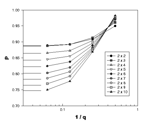
Figure 8.4: Probability of finding a state $\rho$ (for systems of $2\times N_{2}$ dimensions) which has its two conditional $q$-entropies of a positive nature vs. $1/q$. Different curves correspond to different dimensions. The monotonic decreasing behaviour of these probabilities is apparent. The lines are just a guide for the eye. All quantities depicted are dimensionless.

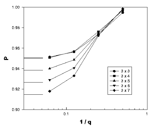
Figure 8.5: Same as in Fig.8.4, but for systems in $3\times N_{2}$ dimensions. All quantities depicted are dimensionless.

Thus far we have considered specific systems for which one of the parties has fixed dimension while that of its partner augments. But what if we consider the case of composite systems with $N_{1}=N_{2}=D$ (that is, two-qudits systems)?. It was already shown in [196], and as we shall see in the forthcoming section, for the case $q=\infty$ that the concomitant probabilities of finding states complying with the classical entropic inequalities (that is, having positive both conditional q-entropies) exhibit a behaviour that is quite different from the one previously discussed. Indeed, the numerical evidence gathered for $q=\infty$ in [196] suggests that, for an $N_{1}\times N_{2}$-composite system of increasing dimensionality, the probability trends that interest us here are clearly different if one considers either (i) increasing dimension for one of the subsystems and constant dimension for the other, or (ii) increasing dimension for both subsystems. In case (i) we have that, for $q=\infty$, the probabilities of finding states with positive conditional $q$-entropies diminish as $N$ grows. In the present effort we have extended the study of case (i) to finite values of $q$, obtaining a similar type of behaviour for $q$-values above a certain special value $q^{*}$. In case (ii) the probability of finding states complying with the classic entropic inequalities steadily grows with $N$ and approaches unity as $N\rightarrow\infty$. The reader is referred to the forthcoming Fig.8.15. The evolution of the probabilities for systems with $N=D\times D$ for finite $q$ does not qualitatively differ from that pertaining to the limit case $q\rightarrow\infty$. As far as monotonicity is concerned, these probabilities share the monotonic behaviour (with $q$) so far discussed for a fixed dimension.

We will now look at two-qudits systems from the following, different perspective: instead of considering the probability of states having positive conditional entropies for both parties, consider the behaviour, as a function of the entropic parameter $q$, of the global probability that an arbitrary state of a two-qudit systems exhibits either (i) both a positive conditional $q$-entropy and a positive partial transpose, or, (ii) both a negative conditional $q$-entropy and a non positive partial transpose. That is, we now focus attention on the probability that i) Peres’ PPT criterion and ii) the signs of the conditional $q$-entropies (regarded as the basis of a separability criterion), both lead to the same answer as far as separability or entanglement are concerned.

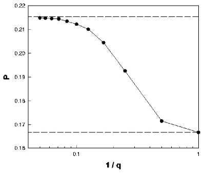
Figure 8.6: Probability (as a function of $q$) of finding a two-qudits state ($D\times D,D=3$) which is characterized by either i) positive conditional $q$-entropy and positive partial transpose, or ii) a negative conditional $q$-entropy and a non positive partial transpose. As $q$ grows so does the degree of agreement with the PPT-criterion, from the von Neumann ($q=1$) case to the “best” $q\rightarrow\infty$ improves. The lines are just a guide for the eye. All quantities depicted are dimensionless.

Fig.8.6 illustrates the case $D=3$ ($N=3\times 3$). We depict there the referred to probabilities as a function of $1/q$, for values of $q\in[2,20]$. Keeping also in mind the results plotted in Fig.8.11 in next section (for $D=2$), we conclude that (i) agreement with Peres’ criterion becomes larger in all cases as $q$ increases up to $q=\infty$, and (ii) the largest degree of agreement, achieved in this limit case, rapidly decreases as $D$ augments from its $D=2$-amount (nearly 75 per cent [196]) to the $D=3$-one (Fig. 8.6) of nearly 22 per cent, and further down to the $D=4$-instance in [196] of 4.5 per cent.

8.2 Probabilities of finding states with positive conditional $q$-entropies.

We have see that when one deals with a classical composite system, described by a suitable probability distribution defined over the concomitant phase space, the entropy of any of its subsystems is always equal or smaller than the entropy characterizing the whole system. This is also the case for separable states of a composite quantum system [126, 127]. In contrast, a subsystem of a quantum system described by an entangled state may have an entropy greater than the entropy of the whole system. Then we are naturally led to the entropic inequalities, whose violation provides a clear and direct information-theoretical manifestation of the phenomenon of entanglement.

This section is similar to the previous one, but we extend our results using the so called participation ratio,

$$R(\hat{\rho})\,=\,\frac{1}{Tr(\hat{\rho}^{2})},$$ (8.8)

and the maximum eigenvalue $\lambda_{m}$ of $\rho$ as a degree of mixture, $\rho$ being the density matrix describing the state of the system under consideration. Besides, we derive the proportion of states in $2\times 2$ and $2\times 3$ systems (two-qubits and qubit-qutrit systems) which are separable or unentangled vs. $R$.

We determined numerically, by recourse to the usual Monte Carlo calculation and for different values of the entropic parameter $q$, the probability of finding a two-qubits state which, for a given degree of mixture $R=1/Tr\,(\rho^{2})$, has positive conditional $q$-entropies. The results are depicted in Fig.8.7. The solid line in Fig.8.7 corresponds to the probability of finding, for a given degree of mixture $R=1/Tr\,(\rho^{2})$, a two-qubit state with a positive partial transpose. Since Peres’ criterium for separability is necessary and sufficient, this last probability coincides with the probability of finding a separable state. We see that, as the value of $q$ increases, the curves associated with the conditional entropies approaches the curve corresponding to Peres criterium. However, even in the limit $q\rightarrow\infty$ the entropic curve lies above the Peres’ one by a considerable amount. This means that, even for $q\rightarrow\infty$, there is a considerable volume in state space occupied by entangled states complying with the classical entropic inequalities (that is, having positive conditional entropies).

Figure 8.7: Probability of finding (for different values of $q$) a two-qubits state which, for a given degree of mixture $R=1/Tr\,(\rho^{2})$, has positive relative $q$-entropies. The solid line corresponds to the probability of finding, for a given degree of mixture $R=1/Tr\,(\rho^{2})$, a two-qubits state with a positive partial transpose.

The probability of finding separable states increases with the degree of mixture [186], as it is evident from the solid curve in Fig.8.7. Also, one can appreciate the fact that a similar trend is exhibited by the probability of finding, for a given $q$-value, states with positive conditional $q$-entropies.

We have computed numerically the probability (for different values of $q$) that a two-qubits state with a given degree of mixture be correctly classified, either as entangled or as separable, on the basis of the sign of the conditional $q$-entropies. The results are plotted in Fig.8.8. That is, Fig.8.7 depicts the probability of finding (for different values of $q$) a two-qubits state which, for a given degree of mixture $R=1/Tr\,(\rho^{2})$, either has (i) both conditional $q$-entropies positive, as well as a positive partial transpose, or (ii) has a negative conditional $q$-entropy and a non positive partial transpose. We see that, for all values of $q>0$, this probability is equal to one both for pure states ($R=1$) and for states with ($R>3$). The probability attains its lowest value $P_{m}(q)$ at a special value $R_{m}(q)$ of the participation ratio. Both quantities $R_{m}(q)$ and $P_{m}(q)$ exhibit a monotonic increasing behaviour with $q$, adopting their maximum values in the limit $q\rightarrow\infty$.

Figure 8.8: Probability of finding (for different values of $q$) a two-qubits state which, for a given degree of mixture $R=1/Tr\,(\rho^{2})$, either (i) has both relative $q$-entropies positive, as well as a positive partial transpose, or (ii) has a negative relative $q$-entropy and a non positive partial transpose.

In Fig.8.7 and Fig.8.8 we have used the participation ratio $R$ as a measure of mixedness. The quantity $R$ is, essentially, a $q$-entropy with $q=2$. The $q$-entropies associated with other values of $q$ are legitimate measures of mixedness as well, and have already found applications in relation with the study of entanglement [186, 192]. It is interesting to see what happens, in the present context, when we consider measures of mixedness based on other values of $q$. Of particular interests is the limit case $q\rightarrow\infty$ which, as already mentioned, is related to the largest eigenvalue of the density matrix. The largest eigenvalue constitutes a legitimate measure of mixture in its own right: states with larger values of $\lambda_{m}$ can be regarded as less mixed. Its extreme values correspond to (i) pure states (with $\lambda_{m}=1$) and (ii) the density matrix $\frac{1}{4}\hat{I}$ (with $\lambda_{m}=1/4$). In Figures 8.9-8.10 we have considered (in the horizontal axes) the largest eigenvalue $\lambda_{m}$ as a measure of mixedness. We computed the probability of finding (for different values of $q$) a two-qubits state which, for a given value of the maximum eigenvalue $\lambda_{m}$, has positive conditional $q$-entropies. The results are depicted in Fig.8.9. The solid line corresponds to the probability of finding, for a given degree of mixture $R=1/Tr\,(\rho^{2})$, a two-qubits state with a positive partial transpose. We see in Fig.8.9 that, for $\lambda<1/3$, the probability of finding states verifying the classical entropic inequalities (i.e., having positive conditional entropies) is, for all $q>0$, equal to one. This is so because all states whose largest eigenvalue $\lambda_{m}$ is less or equal than $1/3$ are separable [192].

Figure 8.9: Probability of finding (for different values of $q$) a two-qubits state which, for a given value of the maximum eigenvalue $\lambda_{m}$, has positive relative $q$-entropies. The solid line corresponds to the probability of finding, for a given value of $\lambda_{m}$, a two-qubits state with a positive partial transpose.

Figure 8.10: Probability of finding (for different values of $q$) a two-qubits state which, for a given value of the maximum eigenvalue $\lambda_{m}$, either (i) has its two relative $q$-entropies positive, as well as a positive partial transpose, or (ii) has a negative relative $q$-entropy and a non positive partial transpose.

Fig.8.10 depicts the probability of finding (for different values of $q$) a two-qubits state which, for a given value of the maximum eigenvalue $\lambda_{m}$, either has (i) both conditional $q$-entropies positive and a positive partial transpose, or (ii) a negative conditional $q$-entropy and a non positive partial transpose.

A remarkable aspect of the behaviour of the sign of the conditional $q$-entropies, which transpires from Figures 8.7 and 8.9, is that, for any degree of mixture, the volume corresponding to states with positive conditional $q$-entropies ($q>0$) is a monotonous decreasing function of $q$. This feature interesting because, for a single given state $\rho$, the conditional $q$-entropy is not necessarily decreasing in $q$ [127]. This means that the positivity of the conditional entropy of a given state $\rho$ and for a given value $q^{*}$ of the entropic parameter does not imply the positivity of the conditional $q$-entropies of that state for all $q<q{*}$. That is, $q<q^{*}$ does not imply that the family of states exhibiting positive conditional $q^{*}$-entropies is a subset of the family of states with positive $q$-entropies. This fact notwithstanding, the numerical results reported here indicate that for $0<q<q{*}$ the volume of states with positive $q^{*}$-conditional entropies is smaller than the volume of states with positive $q$-entropies. This implies that, among all the $q$-entropic separability criteria, the one corresponding to the limit case $q\rightarrow\infty$ is the strongest one, as was suggested by Abe in [134] on the basis of his analysis of a monoparametric family of mixed states for multi-qudit systems.

It is interesting to see the behaviour, as a function of the entropic parameter $q$, of the global probability (regardless of the degree of mixture) that an arbitrary state of a two-qubit system exhibits simultaneously (i) a positive conditional $q$-entropy and a positive partial transpose, or (ii) a negative conditional $q$-entropy and a non positive partial transpose. In order words, this is the probability that for an arbitrary state the entropic separability criterium and the Peres’ criterium lead to the same “conclusion” with respect to the separability (or not) of the state under consideration. In Fig.8.11 we depict this probability as a function of $1/q$, for values of $q\in[2,20]$. We see that this probability is an increasing function of $q$. In the limit $q\rightarrow\infty$ this probability approaches the value $0.7428$. On the other hand, for $q=1$ (that is, when we use the standard logarithmic entropy) the probability is approximately equal to $0.6428$.

Figure 8.11: Probability (as a function of $q$) of finding a two-qubits state which either has both positive relative $q$-entropies and a positive partial transpose, or has a negative relative $q$-entropy and a non positive partial transpose.

We have performed for qubit-qutrit systems calculations similar to the ones that we have already discussed for two-qubits systems. The results are summarized in Figures 8.12 and 8.13. Fig.8.12 depicts the probability of finding (for different values of $q$) a qubit-qutrit state which, for a given degree of mixture $R=1/Tr\,(\rho^{2})$, has positive conditional $q$-entropies. The solid line in Fig.8.12 corresponds to the probability of finding, for a given degree of mixture $R=1/Tr\,(\rho^{2})$, a qubit-qutrit state with a positive partial transpose. Fig.8.13 depicts the probability of finding, for different values of $q$, a qubit-qutrit state which has, for a given degree of mixture $R=1/Tr\,(\rho^{2})$, either (i) its two conditional $q$-entropies positive, as well as a positive partial transpose, or (ii) a negative conditional $q$-entropy and a non positive partial transpose. We have also computed the probability (for different values of $q$) that an arbitrary qubit-qutrit state (regardless of its degree of mixture) be correctly classified, either as entangled or as separable, on the basis of the sign of the conditional $q$-entropies. These probabilities are depicted in Fig.8.14, for values of $q$ in the interval $q\in[2,20]$. As happens with two-qubits systems, this probability is an increasing function of $q$. For $q=1$ the probability is equal to $0.3891$ and approaches the (approximate) value $0.4974$ as $q\rightarrow\infty$. For a given value of $q$, the probability of coincidence between the Peres’ and the entropic separability criteria are seen to be smaller in the case of qubit-qutrit systems than in the case of two-qubits systems.

Figure 8.12: Probability of finding (for different values of $q$) a qubit-qutrit state which, for a given degree of mixture $R=1/Tr\,(\rho^{2})$, has positive relative $q$-entropies. The solid line corresponds to the probability of finding, for a given degree of mixture $R=1/Tr\,(\rho^{2})$, a qubit-qutrit state with a positive partial transpose.

Figure 8.13: Probability of finding a qubit-qutrit state which, for a given degree of mixture $R=1/Tr\,(\rho^{2})$, and for different values of $q$, either (i) has its two relative $q$-entropies positive, as well as a positive partial transpose, or (ii) has a negative relative $q$-entropy and a non positive partial transpose.

Figure 8.14: Probability (as a function of $q$) of finding a qubit-qutrit state which either has both positive relative $q$-entropies and a positive partial transpose, or has a negative relative $q$-entropy and a non positive partial transpose.

Finally, we have computed the probabilities of finding states with positive conditional $q$-entropies (for the case $q=\infty$) for bipartite quantum systems described by Hilbert spaces of increasing dimensionality. Let $N_{1}$ and $N_{2}$ stand for the dimensions of the Hilbert spaces associated with each subsystem, and $N=N_{1}\times N_{2}$ be the dimension of the Hilbert space associated with the concomitant composite system. We have considered three sets of systems: (i) systems with $N_{1}=2,3$ and increasing values of $N_{2}$, and (ii) systems with $N_{1}=N_{2}$ and increasing dimensionality. The computed probabilities are depicted in Fig.8.15, as a function of the total dimension $N$. The three upper curves correspond (as indicated in the figure) to composite systems with $N_{1}=2$, $N_{1}=3$, and $N_{1}=N_{2}$. For the sake of comparison, the probability of finding states complying with the Peres partial transpose separability criterium (lower curve) is also plotted. In order to obtain each point in Fig.8.15, $10^{8}$ states were randomly generated.

Some interesting conclusions can be drawn from Fig.8.15. In the case of composite systems with $N_{1}=N_{2}$, the probability of finding states complying with the classical ($q=\infty$) entropic inequalities (that is, having positive both conditional q-entropies) is an increasing function of the dimensionality. Furthermore, this probability seems to approach $1$, as $N\rightarrow\infty$. In other words, Fig.8.15 provides numerical evidence that, in the limit of infinite dimension, two-qudits systems behave classically, as far as the signs of the conditional $q$-entropies are concerned.

When considering composite systems with increasing dimensionality, but keeping the dimension of one of the subsystem constant ($N_{1}=2,3$), we obtained numerical evidence that the probability of having positive conditional $q$-entropies (again, with $q=\infty$) behave in a monotonous decreasing way with the total dimension $N$.

It is interesting to notice that the probabilities of finding states with positive $q$-entropies are not just a function of the total dimension $N=N_{1}\times N_{2}$ (as happens, with good approximation, for the probability of having a positive partial transpose). On the contrary, they depend on the individual dimensions ($N_{1}$ and $N_{2}$) of both subsystems. Furthermore, the trend of the alluded to probabilities are clearly different if one considers composite systems of increasing dimension with either (i) increasing dimensions for both subsystems or (ii) increasing dimension for one of the subsystems and constant dimension for the other one.

Figure 8.15: Global probability of finding a state (pure or mixed) of a bipartite quantum system with positive relative $q$-entropies. $N_{1}$ and $N_{2}$ stand for the dimensions of the Hilbert spaces associated with each subsystem, and $N=N_{1}\times N_{2}$ is the dimension of the Hilbert space associated with the composite system as a whole. The three upper curves correspond (as indicated in the figure) to composite systems of increasing dimensionality, and with $N_{1}=2$, $N_{1}=3$, and $N_{1}=N_{2}$. The probability of finding a state complying with the Peres partial transpose separability ctiterium (lower curve) is also plotted.

8.3 Maximally entangled mixed states (MEMS) viewed in the light of the entropic criterion

Recourse to entanglement is required so as to implement quantum information processes [115] such as quantum cryptographic key distribution [116], quantum teleportation [102], superdense coding [99], and quantum computation [117]. Indeed, production of entanglement is a kind of elementary prerequisite for any quantum computation.

In practice, one will more often have to deal with mixed states than with pure ones. From the point of view of entanglement-exploitation, one should then be interested in maximally entangled mixed states (MEMS) $\rho_{MEMS}$ that have been studied, for example, in Refs. [189, 190] for the two-qubits instance of two (one qubit-)subsystems $A$ and $B$. These MEMS states have been recently achieved experimentally [203]. We will focus attention on this kind of states here.

MEMS for a given $R-$value have the following appearance in the computational basis ($|00\rangle,|01\rangle,|10\rangle,|11\rangle$) [189].

$$\rho_{MEMS}=\left(\begin{array}[]{cccc}g(x)&0&0&x/2\\ 0&1-2g(x)&0&0\\ 0&0&0&0\\ x/2&0&0&g(x)\end{array}\right),$$ (8.9)

with $g(x)=1/3$ for $0\leq x\leq 2/3$, and $g(x)=x/2$ for $2/3\leq x\leq 1$. The change of $g(x)-$regime ensues for $R=1.8$. We will reveal below some physical consequences of this regime-change . Of great importance are also mixed states whose entanglement-degree cannot be increased by the action of logic gates [190] that, again in the same basis, are given by

$$\rho_{IH}=\left(\begin{array}[]{cccc}p_{2}&0&0&0\\ 0&\frac{p_{3}+p_{1}}{2}&\frac{p_{3}-p_{1}}{2}&0\\ 0&\frac{p_{3}-p_{1}}{2}&\frac{p_{3}+p_{1}}{2}&0\\ 0&0&0&p_{4}\end{array}\right),$$ (8.10)

whose eigenvalues are the $p_{i};\,\,(i=1,\ldots,4)$ and $p_{1}\geq p_{2}\geq p_{3}\geq p_{4}$. We call these states the Ishizaka and Hiroshima (IH) [190] ones and their concurrence $C_{IH}$ reads

$$C_{IH}\,=\,p_{1}\,-\,p_{3}\,-\,2\,\sqrt{p_{2}\,p_{4}},$$ (8.11)

a relation valid for ranks $\leq 3$ that has numerical support also if the rank is four [190]. Of course, all MEMS belong to the IH-class. Our goal is to uncover interesting correlations between entanglement and mixedness that emerge when we study these states from the view point of conditional entropies.

8.3.1 Entropic inequalities and MEMS

We begin here with the presentation of our results [204]. A few of them are of an analytical nature. For instance, in the case of all states of the forms (8.10) and/or (8.9), the partial traces $\rho_{A/B}$ over one of the subsystems $A$ or $B$ are equal, i.e., for the reduced density matrices we have $\rho_{A}=\rho_{B}$, which entails $S_{q}(A|B)=S_{q}(B|A)$. Notice that this is a particular feature of these states.

As for the form (8.10), we establish a lower bound to its states’ concurrence for a considerable $R-$range (see Fig.8.18), namely,

$$C_{IH;Min}=[\sqrt{3R(4-R)}-R]/(2R),$$ (8.12)

where $R$ is the participation ratio (8.8). In the case of MEMS and in the vicinity of $R=1$ we can analytically relate entropic changes with concurrence-changes, in the fashion (remember that for MEMS $C\equiv C_{Max}$)

$$\Delta S_{q}(A|B)\,=\,-[2q/\{\ln(2)(q-1)\}]\,\Delta C.$$ (8.13)

The case $q\rightarrow\infty$ is the strongest $q$-entropic criterion [194]. Eq. (8.13) expresses the fact that, for MEMS, small deviations from pure states (for which the $q$-entropic criteria are necessary and sufficient separability conditions) do not change the criteria’s validity, that becomes then extended to a class of mixed states.

Figure 8.16: Plot of the concurrence $C_{IH}$ for the two kinds of maximally entangled states: Ishizaka and Hiroshima ones (with dots) and MEMS vs. $R$ (upper solid curve) for a sample set. Their corresponding $S_{\infty}(A|B)$-values are also shown. Contour lines can be found analytically (see text for details). The entropic criteria always provide in this range the correct answer in order to detect entanglement.

As stated above, we deal with two kinds of maximally entangles states (MEMS and Ishizaka and Hiroshima ones) [204]. We call the class that comprises both kinds the ME-one. Fig.8.16 depicts the overall situation. In the upper part we plot the ME-states’ concurrence (8.11) vs. the participation ratio. $R$ ranges in the interval $1<R<1.8$ (the latter figure corresponds to the above mentioned transition point for MEMS). (A): the upper line gives MEMS-states and the lower one the lower bound (8.12). (B): the lower part of the Figure gives the conditional entropy of the ME states $S_{q}(A|B)$ for $q=\infty$ (the solid curve corresponds to the MEMS case). It is always negative, so that here the entropic inequalities for entangled states yield the expected negative result.

Fig.8.17 is a plot of the concurrence $C_{IH}$ vs. $\lambda_{max}$, the maximum eigenvalue of our ME bipartite states $\hat{\rho}$. The dashed line corresponds to MEMS. The graph confirms the statement made in [189] that the latter are not maximally entangled states if mixedness is measured according to a criterion that is not the $R-$one. Three separate regions (I, II, III) can be seen to emerge. The maximum and minimum (continuous) contour lines are of an analytical character:

• First zone: a) $C_{IH}^{max}=\lambda_{max}$ for $\lambda_{max}\in[1/2,1]$

• b) $C_{IH}^{min}=2\lambda_{max}-1$ for Bell diagonal states.

• Second: a) $C_{IH}^{max}=3\lambda_{max}-1$ for $\lambda_{max}\in[1/3,1/2]$

• b) $C_{IH}^{min}=0$

• Third: All states are separable $C_{IH}=0$.

Our three zones (I, II, III) can be characterized according to strict geometrical criteria, as extensively discussed in [192]. Fig.8.18 is a $C_{IH}$ vs. $R$ plot like that of Fig.8.16, but for an extended $R-$range ($1<R<3$). The pertinent bipartite states (randomly generated according to the ZHSL-measure of Ref. [187, 191] fill a “band”. In Fig.8.18 we focus attention on a special type of bipartite states: those that, being entangled, do fulfill the inequalities (8.6).

For these states, let us call them entangled states with classical conditional entropic behaviour (ESCRE) [204], the quasi-triangular solid line depicts, for each $R$, the maximum degree of entanglement attainable. Interestingly enough, the maximum degree of entanglement for ESCRE obtains at $R=1.8$, which signals the change of regime for MEMS (Cf. (8.9) and commentaries immediately below that equation). This fact gives an entropic meaning to that $R-$value. We can state then that i) whenever the entropic criterium turns out to constitute a necessary and sufficient condition for separability (at $R=1$ and $R=3$), the ESCRE-degree of entanglement is null, and ii) the ESCRE-degree of entanglement is maximal at the Munro et al. change-of-regime $R-$value of 1.8.

Figure 8.17: Plot of the concurrence $C_{IH}$ for the class of maximally entangled states vs. their maximum eigenvalue $\lambda_{max}$ for a sample set of states. The dashed line corresponds to $\rho_{MEMS}$-states. Notice the fact that these states are not maximally entangled if mixedness is not given by $R$. Maximum and minimum contours of $C_{IH}$ are analytical. See text for details.

Figure 8.18: Same as in Fig.8.16, with an extended $R$-range. The lower curve with crosses represents the maximum concurrence for each $R$ for those states which observe the classical entropic inequalities (both positive). The curve presents a maximum at $R=1.8$ and it is null at $R=1,3$ where the entropic criterion is necessary and sufficient. This curve does not exactly match the upper MEMS-curve in the range $[1.8,3)$. This is due to the relative scarcity of the pertinent states (generated randomly according to the ZHSL measure). See text for details.

8.4 Correlations between quantum entanglement and entropic measures

It is our intention here to investigate the degree of correlation between (i) the amount of entanglement $E[\rho_{AB}]$ exhibited by a two-qubits state $\rho_{AB}$, and (ii) the $q$-entropies (or $q$-information measures) of $\rho_{AB}$ (notice that we refer here to the total $q$-entropy of the density matrix $\rho_{AB}$ describing the composite system as a whole. We shall not consider conditional $q$-entropies). It is well known that the amount entanglement and the degree mixture, as measured by the $q$-entropies: $R_{q}$ (Rényi’s) or $S_{q}$ (Tsallis’), of a state $\rho_{AB}$ are independent quantities. However, there is a certain degree of correlation among them. States with an increasing degree of mixture tend to be less entangled. In point of fact, all two-qubits states with a large enough degree of mixture are separable. We want to explore to what extent does the strength of the alluded to correlation depend upon the parameter $q$ characterizing the $q$-entropy used to measure the degree of mixture. In particular, we want to find out if there is a special value of $q$ yielding a better entropy-entanglement correlation than the entropy-entanglement correlations associated with other values of $q$.

Our investigations will be based upon a Monte Carlo exploration of ${\cal S}$: the set of all states, pure and mixed of a two-qubits system, exactly in the same way as previously done. In the present investigation we shall deal with the case $N=4$.

Most recent research efforts dealing with the relationship between the degree of mixture and the amount of entanglement focus on the behaviour, as a function of the degree of mixture, of the entanglement properties exhibited by the set of states endowed with a given amount of mixedness. For instance, they consider the behaviour, as a function of the degree of mixture (as measured, for instance, by $S_{2}$), of the average entanglement of those states characterized by a given value of $S_{2}$. Here we are going to adopt, in a sense, the reciprocal (and complementary) point of view. We are going to study the behaviour, as a function of $C^{2}$, of the entropic properties associated with the set of states characterized by a given value of $C^{2}$. This vantage point will enable us to clarify some aspects of the $q$-dependence of the entanglement-mixedness correlation. In particular, we want to asses, for different $q$-values, how sensitive are the average entropic properties to the value of the entanglement of formation (or, equivalently, to the value of the squared concurrence $C^{2}$).

We computed, as a function of $C^{2}$, the average value of the Rényi entropy $R_{q}$ associated with the set of states endowed with a given value of the squared concurrence $C^{2}$ [205]. The results are exhibited in Fig.8.19 (solid lines), where the mean value $\langle R_{q}\rangle$ is plotted against $C^{2}$, for $q=0.5,\,1,\,2,\,10,$ and $\infty$. As stated, the averages are taken over all the states $\hat{\rho}\in{\cal S}$ that are characterized by a fixed concurrence-value. For all $q$ the average entropies diminish as $C$ grows. This behaviour is consistent with the fact that states of increasing entropy tend to exhibit a decreasing amount of entanglement [186, 191, 192]. As $q$ grows, the average entropy decreases, for any $C^{2}$, although the decreasing tendency slows down for large $q$-values. Many recent efforts dealing with the relationship between $q$-entropies and entanglement were restricted to states $\rho_{\rm Bell}$ diagonal in the Bell basis. For such states, both the $R_{q}$ entropy and the squared concurrence $C^{2}$ depend solely upon $\rho_{\rm Bell}$’s largest eigenvalue, so that $R_{q}$ can be expressed as a function of $C^{2}$. The dashed line in Fig.8.19 depicts the functional dependence of the $R_{\infty}$ Rényi entropy, as a function of $C^{2}$, for two-qubits states diagonal in the Bell basis. It is instructive to compare, in Fig.8.19, the curve corresponding to states diagonal in the Bell basis with the curve corresponding (with $q=\infty$) to all two-qubit states. It can can be appreciated that these two curves, even if sharing the same qualitative appearance, differ to a considerable extent.

Figure 8.19: Average value of the Rényi entropy $\langle R_{q}\rangle$ of all states with a given squared concurrence $C^{2}$, as a function of $C^{2}$, and for several $q$-values (solid lines). The dashed line depicts the functional dependence of the $R_{\infty}$ Rényi entropy, as a function of $C^{2}$, for two-qubits states diagonal in the Bell basis. All depicted quantities are dimensionless.

For the sake of comparison, we plotted in Fig.8.20 the mean value $\langle S_{q}\rangle$ of Tsallis’ entropy, as a function of $C^{2}$, for $q=0.5,\,1,\,2,$ and $10$. Again, for each value of $C^{2}$, the entropy’s average was computed over all those states characterized by that particular $C^{2}$-value. Notice that for large $q$-values, the Tsallis entropy is approximately constant for all $C^{2}$ values, while the Rényi one seems to be much more sensitive in this respect. Entropies tend to vanish for $C^{2}\to 1$, because only pure states can reach the maximum concurrence value. In the inset of Fig.8.20 we depict the behaviour of $\langle S_{q}\rangle_{C^{2}}$ as a function of $1/q$ for a given value of the concurrence ($C^{2}=0.6$), thus illustrating the fact that the mean entropy is a monotonically decreasing function of $q$. For large $q$-values the Tsallis entropy cannot discriminate between different degrees of entanglement for states with $C^{2}<1$, while Rényi’s measure can do it. This fact is related to an important difference between the behaviours, as a function of the parameter $q$, of Rényi’s $R_{q}$ and Tsallis’ $S_{q}$ entropies. The maximum value $R_{q}^{\rm max}$ attainable by Rényi’s entropy (corresponding to the equi-probability distribution) is independent of $q$,

Figure 8.20: Average value of the Tsallis’ entropy $\langle S_{q}\rangle$ of all states with a given squared concurrence $C^{2}$, as a function of $C^{2}$, and for several $q$-values. The inset shows $\langle S_{q}\rangle$ vs. $1/q$ for the particular value of the squared concurrence $C^{2}=0.6$. All depicted quantities are dimensionless.

$$R^{\rm max}_{q}\,=\,-\ln N,$$ (8.14)

where $N$ is the total number of accesible states. On the contrary, the maximum value reachable by the Tsallis entropy $S_{q}$ does depend upon $q$,

$$S^{\rm max}_{q}\,=\,\frac{1-N^{1-q}}{(q-1)}.$$ (8.15)

Clearly, $S^{\rm max}_{q}\rightarrow 0$ for $q\rightarrow\infty$. One may think that the $q$-dependence of $S^{\rm max}_{q}$ may be appropriately taken into account if one considers (instead of Tsallis’ entropy itself), a normalized Tsallis’ entropy (see Fig.8.21),

$$S^{\prime}_{q}=\frac{S_{q}}{S_{q}^{max}},$$ (8.16)

For instance, in the case of two qubits one has,

$$S_{q}^{max}=\frac{1-4^{1-q}}{(q-1)},$$ (8.17)

and we deal then with

$$S^{\prime}_{q}=\frac{1-Tr[\hat{\rho}^{q}]}{1-4^{1-q}}=\frac{1-\{[Tr(\hat{\rho}^{q})]^{1/q}\}^{q}}{1-4^{1-q}}.$$ (8.18)

Consider now the limit $q\rightarrow\infty$ for a density matrix $\hat{\rho}$ corresponding to a state of fixed concurrence $C$. In such a process one immediately appreciates the fact that $[Tr(\hat{\rho}^{q})]^{1/q}\rightarrow\lambda_{max}$, where $\lambda_{max}$ is the largest eigenvalue of $\hat{\rho}^{q}$. Thus, the limiting value we reach is

$$S^{\prime}_{q}\rightarrow[1-(\lambda_{max})^{q}],$$ (8.19)

and we see that this is always equal to unity for all $C^{2}<1$ and vanishes exactly if $C^{2}=1$ (see Fig.8.21). Consequently, even employing the normalized $S^{\prime}_{q}$, the information concerning the entropy-entanglement correlation tends to disappear in the $q\rightarrow\infty$ limit.

Figure 8.21: Average value of the normalized Tsallis entropy $\langle S_{q}\rangle/S_{q{\rm max}}$ vs. $C^{2}$, for several $q$-values. All depicted quantities are dimensionless.

Returning to our discussion of the connection between entanglement and (total) $q$-entropies of bipartite quantum systems, we have seen that Rényi’s entropy is particularly well suited for (i) discussing the $q\rightarrow\infty$ limit and (ii) studying the $q$-dependence of the entropy-entanglement correlations. For these reasons, in the rest of the present contribution we will focus upon Rényi entropy.

We tackle now the question of the dispersion around these entropic averages. Fig.8.22 is a graph of the dispersions

$$\sigma^{(R)}_{q}\,=\,\left[\langle R_{q}^{2}\rangle-\langle R_{q}\rangle^{2}\right]^{1/2},$$ (8.20)

as a function of $C^{2}$, for the same $q$-values of Fig.8.19. We see that the size of the dispersions diminishes rather rapidly as $C^{2}$ increases towards unity. Also, dispersions tend to become smaller as $q$ grows. This suggests that, as $q$ increases, the correlation between $\langle R_{q}\rangle$ and entanglement improves. A similar tendency, but in the case of $S_{q}$, was detected in [206].

Figure 8.22: Dispersion of the Rényi entropy $\sigma^{(R)}_{q}=\left[\langle R_{q}^{2}\rangle-\langle R_{q}\rangle^{2}\right]^{1/2}$ for all qubits states with a given $C^{2}$, as a function of $C^{2}$, and for several $q$-values. All depicted quantities are dimensionless.

In order to estimate in a quantitative the sensitiveness of the average $q$-entropy to changes in the value of $C^{2}$, we computed the derivatives with respect to $C^{2}$ of the average value of Rényi’s entropy associated with states of given $C^{2}$,

$$\frac{d\langle R_{q}\rangle}{d(C^{2})}.$$ (8.21)

In Fig.8.23 we plot the above derivatives, against $C^{2}$, for $q=0.5,1,2,10$, and $\infty$. These derivatives fall abruptly to zero, in the vicinity of the origin, as $C^{2}$ diminishes. As a counterpart, for all $q$, the derivatives exhibit a rapid growth with $C^{2}$ for small values of the concurrence. This growing tendency stabilizes itself and, for $q$ large enough, saturation is reached.

Now let us assume that we know the value of the entropy $R_{q}[\rho]$ of certain state $\rho$. How useful is this knowledge in order to infer the value of $C^{2}$?. In other words, how good is $R_{q}$ as an “indicator” of entanglement? It has been suggested that $q=\infty$ provides a better “indicator” of entanglement than other values of $q$ [206, 207]. There are two ingredients that must be taken into account in order to determine the $q$-value yielding the best entropic “indicator” of entanglement. On the one hand, the sensitivity of the entropic mean value $\langle R_{q}\rangle$ to increments in $C^{2}$, as measured by the derivative $d\langle R_{q}\rangle/d(C^{2})$. On the other hand, the dispersion $\sigma^{(R)}_{q}$, given by (8.20). A given $q$-value would lead to a good entropic “indicator” if it corresponds to (i) a large value of $d\langle R_{q}\rangle/d(C^{2})$, and (ii) a small value of $\sigma^{(R)}_{q}$. These two factors are appropriately taken into account if we compute the ratio

Figure 8.23: The derivative $d\langle R_{q}\rangle/d(C^{2})$, as a function of the squared concurrence $C^{2}$, for several values of the $q$-parameter. All depicted quantities are dimensionless.

$$r\,=\,\left|\frac{\sigma^{(R)}_{q}}{d\langle R_{q}\rangle/d(C^{2})}\right|,$$ (8.22)

between the dispersions depicted in Fig.8.22 and the derivative of Fig.8.23. The ratio $r$ provides a quantitative measure for the strength of the entropic-entanglement correlations. The quantity $r$ constitutes an estimate of the smallest increment $\Delta C^{2}$ in the squared concurrence which is associated with an appreciable change in $R_{q}$. In order to clarify this last assertion, an analogy with the uncertainty associated with the measurement of time in quantum mechanics can be established. Let us assume that we can measure an observable $\hat{A}$. Then, the time uncertainty $\Delta t$ depends upon two quantities, (i) the time derivative of the expectation value of the observable, $d\langle\hat{A}\rangle/dt$, and (ii) the uncertainty of the observable, $\Delta\hat{A}=[\langle\hat{A}^{2}\rangle-\langle\hat{A}\rangle^{2}]^{1/2}$. The time uncertainty is given by [24]

$$\Delta t\,=\,\frac{\Delta\hat{A}}{d\langle\hat{A}\rangle/dt}$$ (8.23)

The above expression for $\Delta t$ gives an estimation of the smallest time interval that can be detected from measurements of the observable $\hat{A}$. In the analogy we want to establish, $C^{2}$ plays the role of $t$, and $R_{q}$ plays the role of the observable $A$. The ratio $r$ is depicted in Fig.8.24, as a function of $C^{2}$, for $q=1$ and $q=\infty$. The two upper curves in Fig.8.24 correspond to the $r$-values obtained when all the states in the two-qubits state-space ${\cal S}$ are considered. On the other hand, the lower curves are the ones obtained when the computation of $r$ is restricted to states diagonal in the Bell basis. When all states in ${\cal S}$ are considered, the values of $r$ associated with $q=\infty$ are seen to be smaller than the values corresponding to $q=1$, which can be construed as meaning that the $q$-entropies with $q=\infty$ can indeed be regarded as better “indicators” of entanglement than the $q$-entropies associated with finite values of $q$, as was previously suggested in [206, 207]. Alas, the results depicted in Fig.8.24 indicate that this improvement of the entropy-entanglement correlation associated with $q=\infty$ is not considerable. The usefulness of $q$-entropies with $(q\rightarrow\infty)$ as an “indicator” of entanglement was proposed in [207] on the basis of the behaviour of states diagonal in the Bell basis. As already mentioned, the squared concurrence $C^{2}$ of states $\rho_{\rm Bell}$ diagonal in the Bell basis can be expressed as a function of $R_{\infty}$, since both these quantities depend solely on the largest eigenvalue $\lambda_{m}$ of $\rho_{\rm Bell}$ (in particular, $R_{\infty}=-\ln\lambda_{m}$). This means that, as pointed out in [206, 207], for states diagonal on the Bell basis there is a perfect correlation between $C^{2}$ and $(q\!=\!\infty)$-entropies (and, consequently, $r$ vanishes). This implies that, when restricting our considerations only to states diagonal in the Bell basis, the entropy-entanglement correlation is much more strong for $q=\infty$ than for other values of $q$. States diagonal in the Bell basis are important for many reasons, but their properties are by no means typical of the totality of the state-space ${\cal S}$. See for instance, as depicted in Fig.8.24, the behaviour of $r$ (for $q=1$) associated with (i) all states in ${\cal S}$ and (ii) states diagonal in the Bell basis. There are remarkable differences between the two cases.

Figure 8.24: The absolute value of the quotient $r=\left|\frac{\sigma^{(R)}_{q}}{d\langle R_{q}\rangle/d(C^{2})}\right|$, as a function of the squared concurrence $C^{2}$, for $q=1$ and $q=\infty$. The two upper curves correspond to all states in the two-qubit state-space ${\cal S}$. The lower curves correspond to states diagonal in the Bell basis. All depicted quantities are dimensionless.

We thus find ourselves in a position to assert that the relationship between the $q$-entropies and the amount of entanglement exhibited by the family of states diagonal in the Bell basis does not constitute a reliable guide to infer the typical behaviour of states in the two-qubits state-space ${\cal S}$ [205]. When considering the complete state-space ${\cal S}$, the ${q\!=\!\infty}$-entropies turn out to be only a slightly better, as entanglement “indicators”, than the entropies associated with other values of $q$.

8.5 Concluding remarks

In this Chapter we have extensively explored all possible connections of the so called $q$-entropic information measures and their connection with entanglement. We have first explored in composite bipartite systems the features relevant to a family of these entropies, the conditional $q$-entropies, in terms of the total volume occupied by those states which do not violate the classical entropic inequalities. These inequalities constitute a necessary criterion for clearing up the separability of a given mixed state $\rho$, being also sufficient for pure states. Secondly, the connection with entanglement and mixedness has been also studied along similar lines. Also, we focused our attention on the interesting properties that link a particular class of states, the so called Maximally Entangled Mixed States (MEMS), with the violation of the former entropic inequalities. Finally, we showed that there exist a direct correlation between average entropies for a given value of the concurrence and this measure of entanglement, for different values of the entropic parameter $q$.

We then conclude that [194, 196, 204, 205]

• After a systematic survey of the space of pure and mixed states of bipartite systems of arbitrary dimension, the monotonicity with $q$ of both the Tsallis and Rényi entropies has been analyzed for two-qubits and a qubit-qutrit system, for different values of the rank of the pertinent (mixed state) statistical operator $\rho$. In spite of the fact that most states have a Tsallis or Rényi conditional entropy behaving in a monotonic fashion with $q$, the proportion of these states always diminishes as the rank of the state $\rho$ decreases, regardless of the dimension of the system and the conditional entropy used. The proportion of states with a monotonous conditional entropy is larger for the case of the Tsallis information measure.

  Concerning the volumes in state-space associated with states complying with the “classical” entropic inequalities, we have presented results for states of dimensions $2\times 2$ up to $2\times 10$ and for states ranging from $3\times 3$ to $3\times 7$. In general, the volume occupied by states with positive conditional $q$-entropies (for a given $q$) is not a function solely of the total dimension $N=N_{1}\times N_{2}$. Instead, it depends on both subsystems’ dimensions, $N_{1}$ and $N_{2}$. For a given fixed value of $N_{1}=2,3$, and for $q$-values above a special value $q^{*}$ (which itself depends upon $N_{1}$), the alluded to volume decreases in a monotonous way with $N_{2}$.

  In addition, the behaviour of two-qudits systems of dimension $3\times 3$ and $4\times 4$ has also been taken into account. In all these cases, our numerical results indicate that the probability of finding states endowed either with (i) positive conditional $q$-entropies and a positive partial transpose, or (ii) negative conditional $q$-entropies and a non positive partial transpose, increase in a monotonic way with $q$. However, the largest value of this probability (corresponding to $q=\infty$) diminishes in a very fast fashion with $D$.

  Finally, we computed the volumes (for composite systems with Hilbert space dimensions $2\times N_{2}$ and $3\times N_{2}$) occupied by states complying with the majorization separability criterion, and compared them with the volumes corresponding to states endowed with positive $(q=\infty)$-conditional entropies. The qualitative behaviour (as a function of $N_{2}$) of the volumes associated with states complying (i) with the majorization condition and (ii) with the classical, $(q=\infty)$-conditional entropic inequalities, turned out to be qualitatively alike (and very close to each other in the case of systems of dimension $3\times N_{2}$).

• We have determined, as a function of the degree of mixture, and for different values of the entropic parameter $q$, the volume in state space occupied by those states characterized by positive values of the conditional $q$-entropy. We also computed, for different values of $q$, the global probability of classifying correctly an arbitrary state of a two-qubits system (either as separable or as entangled) on the basis of the signs of its conditional $q$-entropies. This probability exhibits a monotonous increasing behaviour with the entropic parameter $q$. The approximate values of these probabilities are $0.6428$ for $q=1$ and $0.7428$ in the limit $q\rightarrow\infty$.

  An interesting conclusion that can be drawn from the numerical results reported here is that, notwithstanding the known non monotonicity in $q$ of the conditional $q$-entropies [127], the volume corresponding to states with positive conditional $q$-entropies ($q>0$) is, for any degree of mixture, a monotonous decreasing function of $q$.

  Similar calculations were performed for qubit-qutrit systems and for composite systems described by Hilbert spaces of larger dimensionality. We pay particular attention to the limit case $q\rightarrow\infty$. Our numerical results indicate that, for composite systems consisting of two subsystems characterized by Hilbert spaces of equal dimension $N_{1}$, the probability of finding states with positive $q$-entropies tend to 1 as $N_{1}$ increases. In oder words, as $N_{1}\rightarrow\infty$ most states seem to behave (as far as their conditional $q$-entropies are concerned) classically.

• The maximally entangled states of Munro, James, White, and Kwiat [189] are shown to exhibit interesting features vis à vis conditional entropic measures. The same happens with the Ishizaka and Hiroshima states [190], whose entanglement-degree can not be increased by acting on them with logic gates. Maximally entangled states with classical entropic behaviour are seen to exist in the space of two qubits. Special meaning can be assigned to the Munro et al. special participation ratio of 1.8. For entangled states with classical conditional entropic behaviour (ESCRE), the maximum degree of entanglement attainable obtains at $R=1.8$. Even though the entropic criteria are not universally valid for all two-qubits states (yielding only a necessary condition for separability), they have been shown here to preserve their full applicability for an important family of states, namely, those with cannot increase their entanglement under the action of logic gates for participation rations in the interval ($R\in[1,1.8]$). This in turn, gives an entropic meaning to this special $R-$value encountered by Munro et al. [189]. We find explicit “boundaries” to $C_{IH}$ when we express the degree of mixture using the maximum eigenvalue $\lambda_{max}$ of $\rho^{IH}$. It would seem that the characterization of the entanglement for these states, using the $\lambda_{max}$ criterion, provides the best insight into the entanglement features of these states. Beyond a certain value for the participation ratio, namely, $R=1.8$, all states, not necessarily the ones considered before, can be correctly described by the entropic inequalities as far as this criterion is concerned. One may argue that if the quantum correlations are strong enough (greater than $C^{max}_{R=1.8}$ or $C^{max}_{\lambda_{max}=\frac{2}{3}}$), there is still room for entropic-based separability criteria to hold.

• By recourse to the same Monte Carlo procedure as before, we have studied the $q$-dependence of the correlations exhibited by two-qubits states between (i) the amount of entanglement and (ii) the $q$-entropies. It was previously conjectured by other researchers, on the basis of the study of states diagonal in the Bell basis, that the $q$-entropies associated with $q=\infty$ are better “indicators” of entanglement than the entropies corresponding to finite values of $q$. In other words, it was suggested that the $q$-entropy with $q=\infty$ exhibits a stronger correlation with entanglement than the other $q$ entropies. By a comprehensive numerical survey of the complete (pure and mixed) state-space of two-qubits, we have shown here that the alluded to conjecture is indeed correct. However, when globally considering the whole state-space the advantage, as an entanglement indicator, of $(q\!=\!\infty)$-entropy turns out to be much smaller than what can be inferred from the sole study of states diagonal in the Bell basis. This constitutes an instructive example of the perils that entails trying to infer typical properties of general two-qubits states from the study of just a particular family of states, such as those diagonal in the Bell basis.

Chapter 9 Entanglement, $q$-entropies and mixedness

The amount of entanglement and the purity of quantum states of composite systems exhibit a dualistic relationship. As the degree of mixture increases, quantum states tend to have a smaller amount of entanglement. In the case of two-qubits systems, states with a large enough degree of mixture are always separable [186]. A detailed knowledge of the relation between the degree of mixture and the amount of entanglement is essential in order to understand the limitations that mixture imposes on quantum information processes such as quantum teleportation or quantum computing. To study the relationship between entanglement and mixture we need quantitative measures for these two quantities. The entanglement of formation provides a natural quantitative measure of entanglement with a clear physical motivation. As for mixedness, there are several measures of mixture that can be useful within the present context. The von Neumann measure

$$S_{1}\,=\,-Tr\left(\hat{\rho}\ln\hat{\rho}\right),$$ (9.1)

is important because of its relationship with the thermodynamic entropy. On the other hand, the so called participation ratio,

$$R(\hat{\rho})\,=\,\frac{1}{Tr(\hat{\rho}^{2})},$$ (9.2)

is particularly convenient for calculations [186, 189]. The $q$-entropies, introduced in Chapters 4 and 8, which are functions of the quantity

$$\omega_{q}\,=\,Tr\left(\hat{\rho}^{q}\right),$$ (9.3)

provide one with a whole family of measures for the degree of mixture. In the limit $q\rightarrow 1$ these measures incorporate (9.1) as a particular instance. On the other hand, when $q=2$ they are simply related to the participation ratio (9.2).

Next in the present Chapter we study some aspects of the relationship between entanglement and purity, using the $q$-entropies as measures of mixture [192]. In particular, we derive analytically the probability (density) $F(R)$ to find a two qubit state with participation ratio $R$. Several distributions for higher bipartite systems are obtained numerically, and some analytical results are found. We shall also discuss in detail the limit case $q\rightarrow\infty$ and its connection with the use of the largest eigenvalue of $\hat{\rho}$ as a measure of the degree of mixture. For $q\in[2,\infty)$, we obtain analytically the values of the $q$-entropies above which all states are separable. Finally, we derive the analytic probability distribution to find a qubit-qutrit state endowed with a maximum eigenvalue $\lambda_{m}$ and expose the general geometric framework for deriving equivalent distributions in arbitrary bipartite systems of dimension $N=N_{A}\times N_{B}$.

9.1 Distribution of two-qubits states according to their mixture

As described in Sec. (7.1), the space ${\cal S}$ of all (pure and mixed) states of a quantum system described by an $N$-dimensional Hilbert space can be regarded as a cartesian product space ${\cal S}={\cal P}\times\Delta$, where $\cal P$ stands for the family of all complete sets of ortonormal projectors $\{\hat{P}_{i}\}_{i=1}^{N}$, $\sum_{i}\hat{P}_{i}=I$ ($I$ being the identity matrix), and $\Delta$ is the set of all real $N$-tuples $\{\lambda_{1},\ldots,\lambda_{N}\}$, with $\lambda_{i}\geq 1$ and $\sum_{i}\lambda_{i}=1$. A detailed description of the space ${\cal S}$ can be found in Appendix B. It suffices here to mention that the natural measure

$$\mu=\nu\times{\cal L}_{N-1}$$ (9.4)

is the one used in the random generation of two-qubits states ($N=4$). Also, in order to study the distribution of two-qubit states according to their degree of mixture, we identify the simplex $\Delta$ with a regular tetrahedron of side length 1, in ${\cal R}^{3}$, centred at the origin. The mapping connecting the points of the simplex $\Delta$ (with coordinates $(p_{1},\ldots,p_{4})$) with the points $\bf r$ of the tetrahedron is given explicitly in Appendix C. Next we consider two special $q$-cases that are relevant in our study.

9.1.1 The case $q=2$

In this case the degree of mixture is characterized by the quantity $\omega_{2}=Tr(\hat{\rho}^{2})=\sum_{i}p_{i}^{2}$. This quantity is related to the distance $r=\mid{\bf r}\mid$ to the centre of the tetrahedron $T_{\Delta}$ by

$$r^{2}\,=\,-\frac{1}{8}\,+\,\frac{1}{2}\omega_{2}.$$ (9.5)

Thus, the states with a given degree of mixture lie on the surface of a sphere of radius $r$ concentric with the tetrahedron $T_{\Delta}$. See Appendix C for details.

The volume associated with states endowed with a value of $\omega_{2}$ lying within a small interval $dw_{2}$ is clearly associated with the volume $dV$ of the subset of points in $T_{\Delta}$ whose distances to the centre of $T_{\Delta}$ are between $r$ and $r+dr$, with $rdr=\omega_{2}\,d\omega_{2}$. Let $\Sigma_{r}$ denote the sphere of radius $r$ concentric with $T_{\Delta}$. The volume $dV$ is then proportional to the area $A(r)$ of the part of $\Sigma_{r}$ which lies within $T_{\Delta}$. In order to compute the aforementioned area, it is convenient to separately consider three different ranges for the radius $r$.

Let us first consider the range of values $r\in[0,h_{1}]$, where $h_{1}={1\over 4}\sqrt{2\over{3}}$ is the radius of a sphere tangent to the faces of the tetrahedron $T_{\Delta}$. In this case the sphere $\Sigma_{r}$ lies completely within the tetrahedron $T_{\Delta}$. Thus, the area we are interested in is just the area of the sphere,

$$A_{I}(r)=4\pi r^{2}.$$ (9.6)

We now consider a second range of values of the radius, $r\in[h_{1},h_{2}]$, where $h_{2}={\sqrt{2}\over 4}$ denotes the radius of a sphere which is tangent to the sides of the tetrahedron $T_{\Delta}$. In this case, the area of the portion of $\Sigma_{r}$ which lies within $T_{\Delta}$ is

$$A_{II}(r)=4\pi\left[r^{2}-2r(r-h_{1})\right].$$ (9.7)

Finally, we consider the range of values $r\in[h_{2},h_{3}]$, where $h_{3}={\sqrt{6}\over 4}$ is the radius of a sphere passing through the vertices of $T_{\Delta}$. In this case the area $A_{III}$ of the part of the sphere $\Sigma_{r}$ lying within $T_{\Delta}$ is

$$A_{III}(r)=4(S_{A}-3S_{B}),$$ (9.8)

where

$$S_{A} = r^{2}(3\alpha-\pi),$$ (9.9)

$$S_{B} = r^{2}\left[h(-\pi+2\sin^{-1}(C_{1}C_{2}))+2\sin^{-1}\sqrt{1-C^{2}_{1}C^{2}_{2}\over 1+C^{2}_{2}}\right].$$ (9.10)

The quantities appearing in the right hand sides of the above expressions are defined by

$$\alpha=\cos^{-1}\left[{\cos A-\cos^{2}A\over\sin^{2}A}\right];\,\,\,\,A=2\sin^{-1}(D_{1}/r);\,\,\,\,D_{1}={1\over 2}\left({1\over 2}-\sqrt{r^{2}-{1\over 8}}\right),$$ (9.11)

and

$$h = h_{1}/r;\ \ C_{1}={h\over\sqrt{1-h^{2}}};\ \ C_{2}={C_{B}\over\sqrt{1-C^{2}_{B}}};$$ (9.12)

$$C_{B} = \sqrt{D^{2}_{2}-D^{2}_{1}\over r^{2}-D^{2}_{1}};\ \ D_{2}=r\sqrt{1-h^{2}}.$$ (9.13)

Using the relation between $r$ and the participation rate $R=1/Tr(\rho^{2})$,

$$r^{2}=-{1\over 8}+{1\over 2R},$$ (9.14)

we analytically obtained the probability $F(R)$ of finding a quantum state with a participation rate $R$,

$$F(R)\,=\,f(r)\left|\frac{dr}{dR}\right|,$$ (9.15)

Figure 9.1: Probability (density) $P(R)$ of finding two-qubits states with a given amount of mixedness $R$. The solid line corresponds to all states and the dashed line to those ones which are separable only, given by $P_{sep}(R)$. This curve is normalized to the overall probability of finding a separable state so that both $P(R)$ and $P_{sep}(R)$ can be compared at the same scale. The maximum occurs at the separability border $R=3$.

where $f(r)=A(r)/({\rm Volume}[T_{\Delta}])$, and $A(r)$ is given by equations (9.6-9.8). The plot of $F(R)$ is depicted in Fig.9.1. The distribution $F(R)$ was first determined numerically by Zyczkowski et al. in [186]. Here we compute $F(R)$ analytically [192] and, as expected, the calculations coincide with the concomitant numerical results and the ones reported in [186].

Information-theoretical approach to entanglement and $R$

According to the $R-$value, two zones are clearly to be distinguished. In Fig.9.1, entanglement is to be encountered only in the zone lying at the “west” ($R<3$) of the graph. As matter of fact, Fig.9.2 depicts, for several values of the participation ratio $R$, the probability $P_{R}(C^{2})$ of finding in our 15-dimensional space $\mathcal{S}$ of two-qubits a bipartite state of concurrence squared $C^{2}$ (5.23). The inset is a $\langle C^{2}\rangle$ vs. $R$ plot. It is well known that i) no entanglement exists for $R>3$ and ii) $R=1$ only for pure states. It is clear that $R$ plays an important role in pre-determining the possibility of finding entanglement. Obviously, to each curve $P_{R}(C^{2})\,$vs.$\,C^{2}$ one can assign a Shannon information measure

$$S_{R}=-\int_{0}^{1}\,dC^{2}\,P_{R}(C^{2})\,\ln{[P_{R}(C^{2})]},$$ (9.16)

that measures the informational amount contained in the distribution $P_{R}(C^{2})$. If we, in turn, plot now $S_{R}$ vs. $R$, we establish a correlation between the participation ratio and our knowledge regarding the entanglement-distribution (ED) in $\mathcal{S}$. This is done in Fig.9.3, that is a logarithmic plot. In the vertical axis we have the logarithm of the information gain $G=[S_{R}-H_{max}]/S_{R=1}$ (with reference to the uniform distribution, that always entails maximum ignorance). For pure states ($R=1$) $S_{R=1}$ is large, but it does not reach the uniform value $H_{max}$. As stated, we calibrate the information (or ignorance) units so that $G=1$ corresponds to the ignorance concerning the ED for bipartite pure states. It is clearly seen that, as $R$ grows, $G$ steadily increases. We can assert, for instance, that if $R=1.5$, our information gain amounts to $\sim 10$ times the one that we possess at $R=1$. The upper, dashed horizontal line indicates the information gain corresponding to the knowledge, with reference to our 15-dimensional space, of the probability $P(C^{2})$ for all states, mixed or not (See for instance [192]). Of course, we are gaining information because of the known fact that the number of entangled states diminishes with $R$.

Figure 9.2: Probability (density) $P_{R}(C^{2})$ of finding two-qubits states (generated according to the $\mu_{Z}$-measure) with fixed degree of mixture $R$, and endowed with a given value of the concurrence squared $C^{2}$. The range of available values for $C^{2}$ continuously decreases as we approach the limiting value $R=3$. The inset shows the evolution of $C^{2}$ vs. $R$.

Figure 9.3: $\ln{G}$ vs. $R-$plot, with $G=[S_{R}-H_{max}]/S_{R=1}$ the information gain with respect to the uniform distribution $H_{max}$ and $S_{R}$ the information-amount contained in the distribution $P_{R}(C^{2})$ of Fig.9.2. The horizontal dashed line indicates the information gain corresponding to the knowledge of the probability $P(C^{2})$ for all states, mixed or not. The inset shows (again in a logarithmic plot) the evolution of the analogue of a specific heat $C_{R}=R\frac{dG}{dR}$ vs. $R$. A quadratic evolution is observed in the range $\in[1,2]$, which becomes steeper in $\in[2,3]$.

Let us recall here that for a continuous probability distribution (cpd) the entropy is defined only up to an arbitrary additive constant. Only entropy differences do make sense (the information gain is obtained with respect to $H_{max}$). Also, for cpd’s, these differences can become infinite, because one needs an infinite informational amount to pick up a point in the continuum.

The general $F(R)$ in $N=N_{A}\times N_{B}$ dimensions

We have just obtained the distribution $F(R)$ vs. $R$ for two-qubits ($N=4$), under the assumption that they are distributed according to measure (9.4). Through a useful analogy, we have mapped the problem into a geometrical one in ${\cal R}^{3}$ regarding interior and common sections of two geometrical bodies. In the previous case we saw that the main difficulty lies in the third region, where the region of the growing sphere inside the tetrahedron is not described by a spherical triangle. The extension to higher dimensions, however, requires a thorough account of the geometrical tools required, but still it is in principle possible. So, one can find the distribution of states according to $R=1/Tr(\rho^{2})$ basically by computing the surface area of a growing ball of radius $r$ in $N-1$ dimensions (sphere) that remains inside an outer regular $N$-polytope $T_{\Delta}$ (tetrahedron) of unit length, excluding the common regions. A $(N-1)$-dimensional sphere can be parameterized in cartesian coordinates

$$x_{1} = r\sin(\phi_{1})\sin(\phi_{2})\sin(\phi_{3})\,...\,\sin(\phi_{N-3})\sin(\phi_{N-2})$$

$$x_{2} = r\sin(\phi_{1})\sin(\phi_{2})\sin(\phi_{3})\,...\,\sin(\phi_{N-3})\cos(\phi_{N-2})$$

$$x_{3} = r\sin(\phi_{1})\sin(\phi_{2})\sin(\phi_{3})\,...\,\cos(\phi_{N-3})$$

$$...$$

$$x_{N-2} = r\sin(\phi_{1})\cos(\phi_{2})$$

$$x_{N-1} = r\cos(\phi_{1}),$$ (9.17)

with the domains $0\leq\phi_{j}\leq\pi$ for $1\leq j\leq N-3$ and $0\leq\phi_{N-2}<2\pi$. The definition of the $N$-polytope $T_{\Delta}$ then is required. This problem is not trivial at all, because new geometrical situations appear in the intersection of these two bodies. In point of fact there are $N-2$ intermediate regimes between $R=N$ and $R=1$ appearing at integer values of $R$ (recall the previous two-qubits case), where a change in the growth of interior hyper-surfaces occurs (at the values $r_{i}=\sqrt{(N-R_{i})/2R_{i}N},R_{i}=1,...,N$). In any case we can always generate random states $\rho$ in arbitrary dimensions (see Appendix B) and compute the corresponding $F_{N}(R)$ distributions. This is done in Fig.9.4 for several cases. The relation (9.14) is generalized to $N$ dimensions in the form

Figure 9.4: Plot of the $F_{N}(R)$ distributions of mixed states $\rho$ numerically computed in arbitrary dimensions, generated according to (9.4). As we increase the total dimension $N$, the curves become smoother, in correspondence with our geometric interpretation. See text for details.

$$r^{2}=-{1\over 2N}+{1\over 2R}.$$ (9.18)

The distribution $F_{N}(R),\,R\in[N-1,N]$ can be obtained analytically

$$F_{N}(R)\,\sim\,\frac{1}{R^{2}}\big{[}\frac{1}{R}-\frac{1}{N}\big{]}^{\frac{N-3}{2}}$$ (9.19)

which has been numerically checked. The particular form of $F(R)$ for arbitrary $N$ is difficult to obtain, but nevertheless one can obtain quantitative results for asymptotic values of $N$. It may be interesting to know the position of the maximum of $F(R)$ or the mean value $\langle R\rangle$, which turns to be $\simeq N/2$ [208] for states $\rho$ generated according to (9.4). There is the so called Borel lemma [209] in discrete mathematics that asserts that (translated to our problem) when you grow a $(N-1)$-ball inside $T_{\Delta}$, from the moment that it swallows, say, 1/2 of the volume of it, then the area outside drops very quickly with further grow. So the maximum intersection with the sphere should be approximately for the radious $r^{*}$ where the volume of the ball $V_{N-1}$ equals that of the $T_{\Delta}$-polytope $V_{T}$. It is then that we can assume that the position of $R(r^{*})\simeq R^{\prime}$ such that $F(R=R^{\prime})$ is maximal. Substituting $r^{*}$ in (9.18), and after some algebra, we obtain the beautiful result

$$\lim_{N\to\infty}\,\frac{1/R(r^{*})}{1/N}\,=\,\frac{2\pi+e}{2\pi}\,\simeq\,1.43.$$ (9.20)

In other words, $F_{N}(1/R)\sim\delta(1/R-1/N)$ for large $N$.

We must emphasize that this type of distributions $F_{N}(R)$ are “degenerated” in some cases, that is, different systems may present identical $F(R)$ distributions (for instance, there is nothing different from this perspective between $2\times 6$ and $3\times 4$ systems). We do not know to what extend these distributions are physically representative of such cases, as far as entanglement is concerned. What is certain is that all states $\rho$ with $R\in[N-1,N]$ possess a positive partial transpose. In point of fact, they are indeed separable, as shown in [210]. We merely mean by this that a state close enough to the maximally mixed state $\frac{1}{N}I_{N}$ is always separable. In other words, states lying on $(N-1)$-spheres with radius $r\leq r_{c}\equiv 1/\sqrt{2N(N-1)}$ are always separable.

9.1.2 The case $q=\infty$

Coming back to two-qubits, the quantity $\omega_{q}$ is not appropriately suited to discuss the limit $q\rightarrow\infty$. However, $\omega_{q}^{1/q}$ does exhibit a nice behaviour when $q\rightarrow\infty$. Indeed, we have

$$\lim_{q\to\infty}\,\left(Tr\rho^{q}\right)^{1/q}\,=\,\lim_{q\to\infty}\,\left(\sum_{i}p_{i}^{q}\right)^{1/q}\,=\,\lambda_{m},$$ (9.21)

where

$$\lambda_{m}=\max_{i}\{p_{i}\}$$ (9.22)

is the maximum eigenvalue of the density matrix $\rho$. Hence, in the limit $q\to\infty$, the $q$-entropies (when properly behaving) depend only on the largest eigenvalue of the density matrix. For example, in the limit $q\to\infty$, the Rényi entropy reduces to

$$S^{(R)}_{\infty}\,=\,-\ln\left(\lambda_{m}\right).$$ (9.23)

It is worth realizing that the largest eigenvalue itself constitutes a legitimate measure of mixture. Its extreme values correspond to (i) pure states ($\lambda_{m}=1$) and (ii) the identity matrix ($\lambda_{m}=1/4$). It is also interesting to mention that, for states diagonal in the Bell basis, the entanglement of formation is completely determined by $\lambda_{m}$ (This is not the case, however, for general states of two-qubits systems).

In terms of the geometric representation of the simplex $\Delta$, the set of states with a given value $\lambda_{m}$ of their maximum eigenvalue is represented by (see Appendix C) the tetrahedron determined by the four planes

$$\lambda_{m}\,=\,2({\bf r}\cdot{\bf r}_{i})\,+\,\frac{1}{4},\,\,\,\,\,\,i=1,\ldots,4.$$ (9.24)

The four vertices of this tetrahedron are given by the intersection points of each one of the four possible triplets of planes that can be selected among the four alluded to planes.

For $q\to\infty$ the accessible states with a given degree of mixture are on the surface of a small tetrahedron $T_{l}$ concentric with the tetrahedron $T_{\Delta}$. We are going to characterize each tetrahedron $T_{l}$ (representing those states with a given value of $\lambda_{m}$) by the distance $l$ between (i) the common centre of $T_{\Delta}$ and $T_{l}$ and (ii) each vertex of $T_{l}$. The volume associated with states with a value of $\lambda_{m}$ belonging to a given interval $\lambda_{m}$ is proportional to the area $A(l)$ of the portion of $T_{l}$ lying within $T_{\Delta}$.

Following a similar line of reasoning as the one pursued in the case $q=2$, we consider three ranges of values for $l$. The first range of $l$-values is given by $l\in[0,h_{1}/3]$. The particular value $l=h_{1}/3$ corresponds to a tetrahedron $T_{l}$ whose vertices are located at the centres of the faces of $T_{\Delta}$. Within the aforementioned range of $l$-values, $T_{l}$ is lies completely within $T_{\Delta}$. Consequently, $A(l)$ coincides with the area of $T_{l}$,

$$A_{I}(l)=24\sqrt{3}l^{2}.$$ (9.25)

The second range of $l$-values corresponds to $l\in[h_{1}/3,h_{1}]$. The area of the part of $T_{l}$ lying within $T_{\Delta}$ is now

$$A_{II}(l)=3\sqrt{3}\left[8l^{2}-{3\over 2}(3l-h_{1})^{2}\right]$$ (9.26)

Finally, the third range of $l$-values we are going to consider is $l\in[h_{1},3h_{1}]$. In this case we have

$$A_{III}(l)={3\over 2}\sqrt{3}(3h_{1}-l)^{2}$$ (9.27)

In a similar way as in the $q=2$ case, the above expressions for $A(l)$ lead to the analytical form of the probability (density) $F(\lambda_{m})$ of finding a two-qubits state with a given value of its greatest eigenvalue,

$$F(\lambda_{m})\,=\,\frac{A(l)}{{\rm Volume}[T_{\Delta}]}\,\left|\frac{dl}{d\lambda_{m}}\right|.$$ (9.28)

Regarding $\omega_{q}^{1/q}$ as a measure of mixture, the probability of finding states with given degrees of mixture is depicted in Fig.9.5, for different values of $q$. In the limit $q\rightarrow\infty$, this probability distribution is given by $F(\lambda_{m})$ (which is included in Fig.9.5). Remarkably enough, as $q$ tends to infinity all discontinuities in the derivative of $F(\lambda_{m})$ disappear. Is seems as in the $\lambda_{m}$-domain the distribution is completely smooth, as opposed to the $R$-domain.

Figure 9.5: Probability $F(w_{q}^{1/q})$ versus $w_{q}^{1/q}=\left(\sum_{i}p_{i}^{q}\right)^{1/q}$ for several $q$ values. The value of $w_{q}^{1/q}$ up to which all the states are separable is also indicated.

9.2 $q$-Entropies and the separability threshold

Quantum states of two-qubits are always separable (that is, their entanglement is equal to zero) if the degree of mixture is high enough. This fact was first demonstrated in [186]. With the aid of $q$-entropies it is possible to give this property of two-qubits states a quantitative expression [192]. For values of the parameter $q$ belonging to the interval $[2,\infty)$, a special value of the $q$-entropy exists such that states with an entropy greater than that particular value are always separable.

Let us consider the subset $\Lambda(q;Z)$ of the simplex $\Delta$ consisting of all the points of $\Delta$ such that

$$\omega_{q}\,=\,\sum_{i=1}^{4}\,p_{i}^{q}\,\leq z.$$ (9.29)

Clearly $\Lambda(q;z)$ is a convex set. In our geometric picture of the simplex, the set $\Lambda(q;z)$ corresponds to a subset of the tetrahedron. Incurring in a minor abuse of notation, we shall design this subset with the same symbol $\Lambda(q;z)$.

It is clear that

$$q>2\,\,\Longrightarrow\,\,\Lambda(q;z)\,\subset\,\Lambda(2;z).$$ (9.30)

Let $z(q)$ denote the particular value of $z$ for which the set $\Lambda(q;z)$ becomes tangent to the faces of the tetrahedron. The points where $\Lambda(q;z(q))$ “kisses” the faces of the tetrahedron are those points (within each of the four faces of the tetrahedron) where the quantity $\omega_{q}$ adopts its minimum value. The minimum of $\omega_{q}$ corresponds to a maximum of a $q$-entropy (for instance, to a maximum of Renyi entropy $S^{(R)}_{q}$). Now, within a face of the tetrahedron one of the $p_{i}$’s vanishes. The maximum of a $q$-entropy then corresponds to the centre of the face, where the three non vanishing $p_{i}$’s are equal to $1/3$. Consequently we have that

$$z(q)\,=\,3\,(1/3)^{q}.$$ (9.31)

Now, for $q=2$, we have $z(2)\,=\,\frac{1}{3}$. This value of $\omega_{2}$ corresponds to a participation ration $R=3$. Consequently, the points belonging to $\Lambda(2;z(2))$ are precisely those with $R\leq 3$, which are always separable. Now, we have,

$$q>2\,\, \Longrightarrow \,\,z(q)\,<\,z(2)$$ (9.32)

$$\Longrightarrow \,\,\Lambda(q;z(q))\,\subset\,\Lambda(q;z(2)),$$ (9.33)

which combined with the inclusion relation (9.30) leads to

$$q>2\,\,\Longrightarrow\,\,\Lambda(q;z(q))\,\subset\,\Lambda(2;z(2)).$$ (9.34)

The above equation implies that all states belonging to $\Lambda(q;z(q))$ are separable. Summing up, we have proved that, for $q\geq 2$, those states with

$$w_{q}\,=\,Tr(\rho^{q})\leq\,3\,(1/3)^{q}$$ (9.35)

are always separable. In terms of the Renyi entropies we then have that, for $q\geq 2$, those states with

$$S^{(R)}_{q}[\hat{\rho}]\,\geq\ln 3,$$ (9.36)

are always separable. In the limit $q\rightarrow 1$ (see Eq.(9.23)), the separability criterium given by equation (9.36) implies that all states whose largest eigenvalue $\lambda_{m}$ is less than $1/3$ are separable.

It is interesting that, expressed in terms of the Renyi entropies, the separability threshold does not depend (for $q\geq 2$) on the value of the parameter $q$. The problem of determining the limit values of the Renyi entropies $S^{(R)}_{q}$ such that states with entropies above them are always separable was first addressed by Zyczkowski et al. in [186], where this problem was studied numerically. On the basis of their numerical results, it was conjectured in the aforementioned paper that the limit value of $S^{(R)}_{q}$ is a decreasing function of $q$. Here we prove that, for $q\geq 2$, this limit value is not dependent on $q$ and is equal to $\ln 3$.

9.3 Analytical distributions of arbitrary states vs. their maximum eigenvalue $\lambda_{m}$. The qubit-qutrit case

As we have seen in previous sections, regarding the maximum eigenvalue $\lambda_{m}$ as a proper degree of mixture one is able to find a geometrical picture analogue to the one of the growing sphere. In that case a nested inverted tetrahedron grows inside the outer tetrahedron representing the simplex of eigenvalues $\Delta$. The generalization to higher bipartite systems is similar to the $R$-case, but far much easier to implement mathematically. As in that case, we have a high degree of symmetry in the problem. The advantage is that one does not deal with curved figures but perfectly flat and sharp surfaces instead. This fact makes the general problem more approachable.

We have seen that the problem of finding how the states of a bipartite quantum mechanical system are distributed according to their degree of mixedness can be translated to the realm of discrete mathematics. If we consider our measure of mixedness to be the maximum eigenvalue $\lambda_{m}$ of the density matrix $\hat{\rho}$ and the dimension of our problem to be $N=N_{A}\times N_{B}$, we compute the distribution of states in arbitrary dimensions by letting an inner regular $N$-polytope $T_{l}$ to grow inside an outer unit length $N$-polytope $T_{\Delta}$, the vertices of the former pointing towards the centre of the faces of the latter. In fact, it can be shown that the radius $l$ of the maximum hypersphere that can be inscribed inside the inner polytope is directly related to $\lambda_{m}$.

By computing the surface area of $T_{l}$ strictly inside $T_{\Delta}$, we basically find the desired probability (density) $F_{N}(\lambda_{m})$ of finding a state $\hat{\rho}$ with maximum eigenvalue $\lambda_{m}$ in $N$ dimensions.

To fix ideas, it will prove useful first to define the vertices of $T_{\Delta}$ and $T_{l}$. In fact it is essential, because we need to deal with elements of cartesian geometry in $N$-dimensions. This vectors are given as

$$\vec{r_{1}} = (-\frac{1}{2},-\frac{1}{2\sqrt{3}},-\frac{1}{4}\sqrt{\frac{2}{3}},...,-\frac{1}{N-1}\sqrt{\frac{N-1}{2N}})$$

$$\vec{r_{2}} = (\frac{1}{2},-\frac{1}{2\sqrt{3}},-\frac{1}{4}\sqrt{\frac{2}{3}},...,-\frac{1}{N-1}\sqrt{\frac{N-1}{2N}})$$

$$\vec{r_{3}} = (0,\frac{1}{\sqrt{3}},-\frac{1}{4}\sqrt{\frac{2}{3}},...,-\frac{1}{N-1}\sqrt{\frac{N-1}{2N}})$$

$$\vec{r_{4}} = (0,0,\frac{3}{4}\sqrt{\frac{2}{3}},..,-\frac{1}{N-1}\sqrt{\frac{N-1}{2N}})$$

$$...$$

$$\vec{r_{N}} = (0,0,0,...,\sqrt{\frac{N-1}{2N}}),$$ (9.37)

with $\sqrt{\frac{N-1}{2N}}$ being the distance from the center to any vertex of this regular $N$-polytope of unit length. One can easily check that $\sum_{i}\vec{r_{i}}=\sum_{i,j}\vec{r_{i}}\cdot\vec{r_{j}}=0$, as required. This particular choice for the position of the vertices of this $N$-simplex is such that it simplifies going from one dimension to the next by adding a new azimuthal axis each time. This vectors comply with the relations

$$\vec{r_{i}}\cdot\vec{r_{j}}\, = \,-\frac{1}{2N}+\frac{1}{2}\delta_{ij},$$ (9.38)

$$\lambda_{m}\, = \,2(\vec{r}\cdot\vec{r_{i}})+\frac{1}{N},\,\,\,\,\,\,\,\,i=1...N,$$ (9.39)

where the last equation is the general form of (9.24).

Once we have a well defined $T_{\Delta}$, to know the coordinates of $T_{l}$ is straightforward. In fact, $T_{l}$ is the reciprocication (see [211]) of $T_{\Delta}$. This means that the coordinates of $T_{l}$ are obtained by reversing the sign of the ones of $T_{\Delta}$, multiplied by a suitable factor (which can be shown to be $\sqrt{2N(N-1)}l$, with $l$ defined as the length between the centre of $T_{l}$ to the centre of any of its faces, which in turn points towards the vertices of $T_{\Delta}$). Thus, we can relate $l$ with $\lambda_{m}$ through a general (9.24)-relation $\lambda_{m}=2\,l\,\sqrt{\frac{N-1}{2N}}+\frac{1}{N}$, such that $\frac{dl}{d\lambda_{m}}=\sqrt{(2N)/(N-1)}/2$.

Figure 9.6: Plot of the $F_{N}(\lambda_{m})$ distributions of mixed states $\rho$ numerically computed in arbitrary dimensions, generated according to (9.4). As we increase the total dimension $N$, the curves tend to peak around $1/N$. See text for details.

Several distributions $F_{N}(\lambda_{m})$ are obtained numerically by generating random states $\rho$ according to (9.4) in Fig.9.6. It becomes apparent that as $N$ grows, the distributions are biased towards $\lambda\simeq 1/N$, in absolute agreement with the result (9.20).

As in the $R$-case, $F_{N}(\lambda_{m})$ is distributed into $N-1$ regions separated at fixed values of $\lambda_{m}^{(i)}=\frac{1}{N-i},\,i=1..(N-2)$. The general recipe for obtaining $F_{N}(\lambda_{m})$ is tedious and long, but some nice general results are obtained. The $F_{N}(\lambda_{m})$-distributions for the ranges a) $\lambda_{m}\in[\frac{1}{N},\frac{1}{N-1}]$ and b) $\lambda_{m}\in[\frac{1}{2},1]$ are general and read

$$F_{I}(\lambda_{m})\, = \,\kappa\frac{N}{(N-2)!}\sqrt{\frac{N-1}{2^{N-2}}}\big{[}\sqrt{2N(N-1)}l(\lambda_{m})\big{]}^{N-2},$$ (9.40)

$$F_{Last}(\lambda_{m})\, = \,\kappa\frac{N}{(N-2)!}\sqrt{\frac{N-1}{2^{N-2}}}\bigg{[}\frac{\sqrt{\frac{N-1}{2N}}-l(\lambda_{m})}{\sqrt{\frac{N}{2(N-1)}}}\bigg{]}^{N-2},$$ (9.41)

respectively, where $\kappa\equiv\frac{dl}{d\lambda_{m}}/{\rm Volume}[T_{\Delta}]$ is introduced for convenience.

For the sake of completeness, we briefly describe the physical case of a qubit-qutrit system $(N=6)$. Defining $r_{i}\equiv\sqrt{\frac{N-1}{2N}}$ and $y_{i}\equiv(l(\lambda_{m})(N-1)-\frac{i}{N-i}r_{i})/(\sqrt{N/2(N-1)})$, in addition to the previous regions (9.40) we obtain

$$F_{II}(\lambda_{m})\, = \,\kappa\big{[}F_{I}(\lambda_{m})/\kappa-\frac{(N-1)N}{(N-2)!}\sqrt{\frac{N-1}{2^{N-2}}}[y_{i=1}]^{N-2}\big{]};$$ (9.42)

$$F_{III}(\lambda_{m})\, = \,\kappa\big{[}F_{II}(\lambda_{m})/\kappa+\frac{2^{9}}{5^{4}}\frac{(N-1)N}{(N-2)!}\sqrt{\frac{N-1}{2^{N-2}}}[y_{i=2}]^{N-2}\big{]};$$ (9.43)

$$F_{IV}(\lambda_{m})\, = \,\kappa\big{[}F_{III}(\lambda_{m})/\kappa-2\frac{3^{4}}{5^{4}}\frac{(N-1)N}{(N-2)!}\sqrt{\frac{N-1}{2^{N-2}}}[y_{i=3}]^{N-2}\big{]},$$ (9.44)

for $\lambda_{m}\in[\frac{1}{5},\frac{1}{4}],[\frac{1}{4},\frac{1}{3}]$, and $[\frac{1}{3},\frac{1}{2}]$, respectively. From the previous formulas one can infer a general induction procedure. Analytical results are in excellent agreement with numerical generations.

9.4 Concluding remarks

In this Chapter we have revisited the relationship between entanglement and purity of states of two-qubits systems, in the light of the $q$-entropies as measures of the degree of mixture [192].

The probability $F$ of finding quantum states of two-qubits with a given degree of mixture (as measured by an appropriate function of $\omega_{q}$) is analytically found for $q=2$ and $q\to\infty$. In the latter case, the $q$-entropies become functions of the statistical operator’s largest eigenvalue $\lambda_{m}$. In point of fact, $\lambda_{m}$ itself constitutes a legitimate measure of mixture. During the derivation of the probability (density) distributions $F_{N}$ of finding a bipartite mixed state in arbitrary dimensions $N=N_{A}\times N_{B}$ with a given degree of mixture, we saw that it is more convenient to use $\lambda_{m}$ instead of $R$. In point of fact, we analytically entend by direct demonstration the separability threshold to $q>2$, when using the $q$-entropies as measures of the degree of mixture. In the limit case $q\to\infty$, we see that states $\rho$ with $\lambda_{m}\leq\frac{1}{3}$ are always separable or, alternatively, whenever the information content of the Rényi entropy $S^{(R)}_{q}(\rho)\geq\ln 3$ the state is unentangled.

In the case $q=2$, we saw that the amount of information concerning entanglement distribution is univocally fixed by the participation ratio $R$, which shows in a more direct way the intimate connexion existing between entanglement and mixedness. In other words, we ascertain the amount of information that, with regards to the distribution of entanglement among the states of our space, accompanies the knowledge of the degree of mixedness. Finally, we have derived explicitly the distribution $F_{N}(\lambda_{m})$ vs. $\lambda_{m}$ for the physical meaningful case of a qubit-qutrit system ($N=6$).

Chapter 10 Structure of the space of two-qubit systems: metrics and entanglement

The two-qubits systems with which we are going to be concerned in this Chapter are the simplest quantum mechanical systems exhibiting the entanglement phenomenon and play a fundamental role in quantum information theory. The concomitant space ${\cal S}$ of mixed states is 15-dimensional and its properties are not of a trivial character. Important features of this space, related to the phenomenon of entanglement, have not yet been characterized in full detail, notwithstanding the existence of many interesting efforts towards the systematic exploration of the space of arbitrary (pure or mixed) states of composite quantum systems that have determined typical features with regards to the phenomenon of quantum entanglement. It is mandatory to stress the fact that i) the majority of states in this space are mixed and ii) that most of the exciting proposals in quantum information theory address mainly pure states, contrary to the usual situation encountered by the experimentalist.

In the present Chapter we undertake a Monte Carlo exploration over the space ${\cal S}$ of two-qubits mixed states in order to elucidate the features of the concomitant structure (in terms of different metrics) related to the issue of entanglement [212]. An ab initio detailed analytical description of the aforementioned structures is not possible because it requires a complete characterization of the “geometry” of states which are invariant under PPT action (that is, $\rho\geq 0\Longrightarrow\rho^{T_{A}}\geq 0$), or simply separable, which is not available up to date. In consequence, we carry out numerical computations by randomly generating states of two-qubits systems according to an appropriate measure, studying the ensuing entanglement properties.

We also focus our attention to the different ways that the space ${\cal S}$ can be generated, discussing the adequacy of several distributions for the simplex $\Delta$ of eigenvalues of $\rho$. Finally, the study of the features of real quantum mechanics is drawn in the context of two-rebits systems [191].

10.1 Metrics and entanglement

The protagonist of the following considerations is the maximally mixed (MM) bipartite state $\rho_{MM}=I/4$. This state is surrounded by a separable ball [210], where all states “close enough” to it are separable. Therefore it becomes apparent that a way to characterize the space of two-qubits is through distances from a given state $\rho$, to the MM-one and ask questions like, for instance, starting from the MM, how far do we have to go to find an entangled state? The volume measure $\mu_{Z}\equiv\mu=\nu\times{\cal L}_{N-1}$ (9.4), thoroughly described in previous Chapters and in Appendix B, is not based upon any distance-measure, and consequently has been criticized by Slater [213, 214, 215, 216] on two grounds: i) it is not associated with the volume element of any monotonic metric and ii) it is over-parameterized because the number of variables it needs to parameterize de convex set of $N\times N$ density matrices $\rho$ is $N^{2}+N-1$ rather than the theoretical minimum number $N^{2}-1$. On the other hand [139], these facts are to be weighted against these other two: the measure $\mu_{Z}$ allows for rapid convergence and provides a simple procedure to investigate different separability criteria for bipartite states, as seen in previous Chapters. Regarding “overparameterization” by $\mu_{Z}$, it is possible to express this measure strictly using $N^{2}-1$ parameters.

It is likely that answers to questions like the one posed before might presumably depend on the choice of volume measure. This is precisely what we investigate. A most appropriate alternative is to base our measure on the distance between density matrices. To such an end, let us survey different aspects that may provide some insight into the structure of two-qubits systems.

A. The Bures distance

Let us describe this measure for the sake of completeness. Given two (not necessarily commuting) density matrices $\rho_{1}$ and $\rho_{2}$, Hübner [217] has found an explicit form for the distance $d_{Bures}$ between them, following well known Bures tenets [218] that apply for density operators. One has

$$d_{Bures}(\rho_{1},\rho_{2})\,=\,\sqrt{2}\,\bigg{[}1\,-\,Tr\,\bigg{(}\big{[}\rho_{1}^{1/2}\rho_{2}\,\rho_{1}^{1/2}\big{]}^{1/2}\bigg{)}\bigg{]}^{1/2}.$$ (10.1)

Let

$$\hat{\rho}_{1}|i\rangle\,=\,a_{i}|i\rangle,$$ (10.2)

be the eigenvalue equation for the statistical operator $\hat{\rho}_{1}$ whose associated density matrix is, of course, $\rho_{1}$, so that

$$\hat{\rho}_{1}^{1/2}\,=\,\sum_{i}a_{i}^{1/2}|i\rangle\langle i|.$$ (10.3)

In this basis, we also have

$$\hat{\rho}_{2}\,=\,\sum_{k,j}b_{k,j}|k\rangle\langle j|,$$ (10.4)

an then the triple product in (10.1) yields an operator $\hat{T}$

$$\hat{T}\,=\,\sum_{i,m}a_{i}^{1/2}b_{i,m}a_{m}^{1/2}|i\rangle\langle m|.$$ (10.5)

It is necessary now to diagonalize $T$ so as to get

$$\hat{T}^{1/2}\,=\,\sum_{\beta}t_{\beta,\beta}^{1/2}|\beta\rangle\langle\beta|,$$ (10.6)

and finally, be in a position to define the Bures distance

$$d_{Bures}(\rho_{1},\rho_{2})\,=\,\sqrt{2}\,\bigg{[}1\,-\,\sum_{\beta}t_{\beta,\beta}^{1/2}\bigg{]}^{1/2}.$$ (10.7)

The Bures distance is a function of the so-called ${\it fidelity}$

$$F(\rho_{1},\rho_{2})\,=\,\Bigl{[}\mbox{Tr}\sqrt{\sqrt{{\rho}_{1}}{\rho}_{2}\sqrt{{\rho}_{1}}}\Bigr{]}^{2}$$ (10.8)

between the two states $\rho_{1}$ and $\rho_{2}$ [219]. The fidelity is a relevant quantity for information processing purposes: It constitutes a generalization to mixed states of the overlap-concept between pure states. Thus, whenever the Bures distance is employed, we also describe the fidelity-degree extant between the maximally mixed state $\rho_{MM}$ and an arbitrary mixed state $\rho$.

Lower and upper bounds for the function $d_{Bures}$ (and, in turn, for the fidelity $F$) vs. $R$ are obtained in analytical fashion. A “band” of Bures distances exist for each $R-$value, that ranges from a minimal up to a maximal $d_{Bures}(R)$. There are three $R$ zones in our bipartite state-space, namely, i) $1\leq R\leq 2$, ii) $2\leq R\leq 3$, and iii) $3\leq R\leq 4$. For each of these zones we consider states that, in the product space $\mathcal{S}$ read, respectively,

1. $\rho_{1}=diag(0,0,x,1-x)$,

2. $\rho_{2}=diag(0,x,x,1-2x)$,

3. $\rho_{3}=diag(x,x,x,1-3x)$.

By setting the condition $Tr(\rho^{2})=1/R$, in the case of $\rho_{1,\,2}$ we get only a physical root for $x$ that corresponds to the maximal distance. For $\rho_{3}$ we get two such roots that yield minimal and maximal values. It is important to stress that the aforementioned states are universal, that is, independent of the generation of ${\cal S}$.

B. Measures and distances

One of our present purposes is to replace the volume measure $\mu_{Z}$ by other volume measures based upon proper distance-definitions. One can then randomly generate states according to volume measures pertaining to these different metrics. Of course, within a given state-generation procedure (that uses a volume measure that may or may not be associated to a given metric) one can still determine distance between states according to different distance-recipes.

One can then generate the simplex $\Delta$ of eigenvalues (a subset of a $(N-1)$-dimensional hyperplane of ${\cal R}^{N}$) using different measures [188, 219], namely,

• $\mu_{Z}$

• A Bures volume measure $\mu_{B}$ induced by the Bures metric (see above) in the simplex of eigenvalues

  $$\mu_{B}(\Delta)\,=\,\frac{2^{N^{2}-N}\Gamma(N^{2}/2)}{\pi^{N/2}\Gamma(1)..\Gamma(N+1)}\frac{\delta(\sum_{j=1}^{N}\lambda_{j}-1)}{\sqrt{\lambda_{1}\lambda_{2}...\lambda_{N}}}\,\prod_{i<j}^{N}\frac{(\lambda_{i}-\lambda_{j})^{2}}{\lambda_{i}+\lambda_{j}}.$$ (10.9)

• A Hilbert-Schmidt (HS) volume measure (induced by the HS metric) in the $\Delta-$simplex of eigenvalues

  $$\mu_{HS}(\Delta)\,=\,\frac{\Gamma(N^{2})\,\delta(\sum_{j=1}^{N}\lambda_{j}-1)}{\prod_{j=0}^{N-1}\Gamma(N-j)\Gamma(N-j+1)}\,\prod_{i<j}^{N}(\lambda_{i}-\lambda_{j})^{2}.$$ (10.10)

Independently of the volume measure choice we can still speak of distances between bipartite states measured according to either

• The Bures distance (10.1) or

• The Hilbert-Schmidt distance

  $$d_{HS}(\rho_{1},\rho_{2})\,=\,\sqrt{Tr[(\rho_{1}-\rho_{2})^{2}]}.$$ (10.11)

C. A random walk

Assume that we are interested in reaching the MM bipartite state $\frac{1}{4}I$, starting from an entangled initial bipartite state $\rho_{0}$. We call ${\mathcal{S}}_{sep}$ the set of separable states ${\mathcal{S}}_{sep}\subset\mathcal{S}$. The task can be performed by following a simulated-annealing minimization-procedure in the 15-dimensional set ${\mathcal{S}}_{sep}$. The ensuing Monte Carlo recipe resembles a “random walk”. One takes advantage of the fact that ${\mathcal{S}}_{sep}$ is a convex set. Thus, optimization is equivalent to a random walk subject to constraints. Our search begins then somewhere in exterior of ${\mathcal{S}}_{sep}$ and we look for a minimal distance $d^{MIN}$ to $\rho_{MM}$. This minimal distance can be either of the Bures ($d_{Bures}$) or of the HS ($d_{HS}$) kind. In view of the fact that all states $\in\mathcal{S}$ are separable for $R>3$, our minimal distance to $\rho_{MM}$ is obtained for a state characterized by a participation ratio $R=3$. Interestingly enough, these minimal distances can be obtained not only numerically but also in analytic fashion. The pertinent results are depicted in Fig.10.1a, where we plot, for the two distances, the ratio $d/d^{MIN}$ vs. number of Monte Carlo (MC) steps. By a MC step we mean a realization of the set of variables that parameterize our two-qubits state $\rho$, consisting in changing the configuration of $\rho$ a reasonably large number of times until “thermalization” is reached. The condition $R=3$ entails finding the appropriate $x$ value for a state that, in the product space $\mathcal{S}$, is of the form $\rho=diag(x,x,x,1-3x)$. Two solutions exist, $x=1/3,1/6$. Choosing the latter, one encounters

Figure 10.1: a) Evolution of the ratio $d/d^{MIN}$ vs. the number of Monte Carlo (MC) steps, as we approach the maximally mixed state $\frac{1}{4}I$ from outside the set ${\mathcal{S}}_{sep}$ of separable states, for the Bures (solid line) and Hilbert-Schmidt (dashed line) distances (see text for details). Convergence with the theoretical value is reached quickly. b) Evolution of the ratio $d/d^{MAX}$ vs. the number of MC steps throughout the interior of ${\mathcal{S}}_{sep}$, for the Bures (solid line) and Hilbert-Schmidt (dashed line) distances. Agreement with predicted values is excellent.

$$d_{Bures}^{MIN} = d_{Bures}(I/4,\rho)\sim 0.26105$$ (10.12)

$$d_{HS}^{MIN} = d_{HS}(I/4,\rho)=\frac{1}{2\sqrt{3}}.$$ (10.13)

Analytic and numerical results are seen to eventually match each other. More importantly, it is seen that which of the two distances one uses is of no importance whatsoever.

Another question that might be profitably asked is the following: without leaving ${\mathcal{S}}_{sep}$, what is the farthest from $\rho_{MM}$ that you can go? Let us call $d^{MAX}$ the concomitant “length”. Again, we will have a Bures and an HS quantity (see Fig.10.1b). It is clear that the most dissimilar (to MM) density matrix is, in the product space $\mathcal{S}$, the state $\rho_{1}=diag(1,0,0,0)$ (or any (diagonal) permutation thereof), which will belong to ${\mathcal{S}}_{sep}$ if a suitable basis is chosen. Our quantities are then distances to such a state from the MM one. We immediately get

$$d_{Bures}^{MAX} = d_{Bures}(I/4,\rho_{1})=1$$ (10.14)

$$d_{HS}^{MAX} = d_{HS}(I/4,\rho_{1})=\frac{\sqrt{3}}{2}.$$ (10.15)

The agreement between the above analytical results and numerical simulations is excellent.

D. Distribution of distances and CNOT gate

Let us concern ourselves with one of the basic constituents of any quantum processing device: quantum logical gates, i.e., unitary evolution operators $\hat{U}$ that act on the states of a certain number of qubits. If the number of such qubits is $m$, the quantum gate is represented by a $2^{m}\times 2^{m}$ matrix in the unitary group $U(2^{m})$. These gates are reversible: one can reverse the action, thereby recovering an initial quantum state from a final one. We shall work here with $m=2$. The simplest nontrivial two-qubits operation is the quantum controlled-NOT, or CNOT (equivalently, the exclusive OR, or XOR) (See Sec.(2.6)). Its classical counterpart is a reversible logical gate operating on two bits: $e_{1}$, the control bit, and $e_{2}$, the target bit. If $e_{1}=1$, the value of $e_{2}$ is negated. Otherwise, it is left untouched. The quantum CNOT gate $C_{12}$ (the first subscript denotes the control bit, the second the target one) plays an important role in both experimental and theoretical efforts that revolve around the quantum computer concept. In a given ortonormal basis $\{|0\rangle,\,|1\rangle\}$, and if we denote addition modulo 2 by the symbol $\oplus$, we have

$$|e_{1}\rangle\,|e_{2}\rangle\rightarrow C_{12}\rightarrow|e_{1}\rangle\,|e_{1}\oplus e_{2}\rangle.$$ (10.16)

In conjunction with simple single-qubit operations, the CNOT gate constitutes a set of gates out of which any quantum gate may be built. In other words, single qubit and CNOT gates are universal for quantum computation. A more detailed account on quantum gates is given in Chapter 11.

Figure 10.2: a) Probability (density) distribution of changes in the Bures distance $d_{Bures}$ between states ($\mu_{Z}$-generated) after the application of a CNOT gate. The set of states upon which the gate acts is divided into i) ZONE I: states with a $d_{Bures}$ (from $\frac{1}{4}I$) $<$ $d_{Bures}^{MIN}$, ii) ZONE II: states with a $d_{Bures}$ (from $\frac{1}{4}I$) $>$ $d_{Bures}^{MIN}$, and iii) all states. These curves coincide at the $d_{Bures}=d_{Bures}^{MIN}$ boundary (see text for details). b) Same plot as before using the Hilbert-Schmidt distance.

In Fig.10.2 we depict the probability $P(d)\,\,vs.\,\,d$ of encountering a giving distance $d$ between initial and final states under the CNOT-action, with $d$ given by either the Bures (10.2a) or the HS (10.2b) definitions. Initial states are generated according to $\mu_{Z}$ and chosen in such a way that their distance to $\rho_{MM}$ is

1. always $<d^{MIN}$ (solid curve)

2. always $>d^{MIN}$ (dashed line)

3. no $d^{MIN}-$criterium is employed (dotted curve).

Notice that if the selected initial state is located at any distance smaller than the $d^{MIN}$, by the application of any unitary transformation like the CNOT gate we always obtain a state inside of the sphere of radius $d^{MIN}$, and consequently $P(d)$ is only different from zero in the interval $\left[0,2d^{MIN}\right]$. If the initial state is outside the sphere of radius $d^{MIN}$, $P(d)$ is non null in the interval $\left[0,2d^{MAX}\right]$ because the final state obtained by using the CNOT-gate is not restricted to a given value of $d$. When we choose random the initial state, the value of $P(d)$ slightly moves to the small $d$ values because the final state obtained using an initial state belonging to zone 1 are always restricted to $d<d^{MIN}$. Finally, it is remarkable that the selection of Bures or Hilbert-Schmidt distances does not seem to produce great differences.

E. Effects of the $\mu-$choice

Figure 10.3: Probability of finding a separable state in the space of all two-qubits $\mathcal{H}$, as measured by the Bures distance $d_{Bures}$ from the maximally mixed state $\frac{1}{4}I$, for three different measures of states in $\mathcal{H}$: i) $\mu_{Z}$ (solid line), ii) $\mu_{Bures}$ (dashed line) and ii) $\mu_{Bures}$ (dot-dashed line). The three curves are all alike, but ii) and iii) are closer (nearly coincide at this scale) to one another (indeed they are metric-based measures).

Let us try to discern differences between randomly generating states ${\in\mathcal{S}}$ either according to i) $\mu_{Z}$, ii) $\mu_{Bures}$, and iii) $\mu_{HS}$. Again, $d$ is the distance between a given state ${\in\mathcal{S}}$ and $\rho_{MM}$ (Here we use only $d_{Bures}$). We compute the probability $P_{sep}$ of Monte Carlo-finding a separable bipartite state as a function of $d_{Bures}$. Our results are given in Fig.10.3. Notice the important fact that $P_{sep}$ does not strongly depend on the $\mu-$choice. In point of fact the curves generated according to the Bures or the Hilbert-Schmidt metrics does not differ from each other as much as the one obtained using $\mu_{Z}$. Nevertheless the differences are very tiny and the overall behaviour of the three curves are quantitatively and qualitatively the same. This is probably the most important result of this Chapter: regardless of the nature of the measure employed in the generation of states, the entanglement properties of the set ${\cal S}$ are basically the same. In other words, the space ${\cal S}_{sep}$ of states which comply with the PPT separability criterion is not highly sensitive to the way the states $\rho$ are distributed in ${\cal S}$.

10.2 Comment on the non uniqueness of the generation of bipartite mixed states. Examples

In the papers by Zyczkowski et al. [186, 187], a basic question regarding a natural measure $\mu$ for the set of mixed states $\rho$ was debated. As described in Secs. (7.1) and (9.1), it is know, the set of all states ${\cal S}$ can be regarded as the cartesian product ${\cal S}={\cal P}\times\Delta$, where $\cal P$ stands for the family of all complete sets of ortonormal projectors $\{\hat{P}_{i}\}_{i=1}^{N}$, $\sum_{i}\hat{P}_{i}=I$ ($I$ being the identity matrix), and $\Delta$ is the set of all real $N$-tuples $\{\lambda_{1},\ldots,\lambda_{N}\}$, with $\lambda_{i}\geq 1$ and $\sum_{i}\lambda_{i}=1$. As discussed in those papers and in Appendix B, it is universally accepted to assume the Haar measure $\nu$ to be the one defined over ${\cal P}$, because of its rotationally-invariant properties. But when it turns to discuss an appropriate measure over the simplex $\Delta$, some controversy arises. In all previous considerations here, we have regarded the Leguesbe measure ${\cal L}_{N-1}$ as being the “natural” one. But one must mention that Slater has argued [213, 214] that, in analogy to the classical use of the volume element of the Fisher information metric as Jeffreys’ prior [220] in Bayesian theory, a natural measure on the quantum states would be the volume element of the Bures metric. The problem lies on the fact that there is no unique probability distribution defined over the simplex of eigenvalues $\Delta$ of mixed states $\rho$. In point of fact, the debate was motivated by the fact that the volume occupied by separable two-qubits states (see Chapter 7) was found in [186] to be greater than $50\%$ ($P_{sep}=0.6312$) using the measure $\mu$, something which is surprising.

One such probability distribution that is suitable for general considerations is the Dirichlet distribution [187]

$$P_{\eta}(\lambda_{1},\ldots,\lambda_{N})\,=\,C_{\eta}\lambda_{1}^{\eta-1}\lambda_{2}^{\eta-1}...\lambda_{N}^{\eta-1},$$ (10.17)

with $\eta$ being a real parameter and $C_{\eta}=\frac{\Gamma[N\eta]}{\Gamma[\eta]^{N}}$ the normalization constant. This is a particular case of the more general Dirichlet distribution. The concomitant probability density for variables $(\lambda_{1},...,\lambda_{N})$ with parameters $(\eta_{1},...,\eta_{N})$ is defined by

$$P_{{\bf\eta}}(\lambda_{1},\ldots,\lambda_{N})\,=\,C_{\bf{\eta}}\lambda_{1}^{\eta_{1}-1}\lambda_{2}^{\eta_{2}-1}...\lambda_{N}^{\eta_{N}-1},$$ (10.18)

with $\lambda_{i}\geq 0$, $\sum_{i=1}^{N}\lambda_{i}=1$ and $\eta_{1},...,\eta_{N}>0$, and $C_{\bf{\eta}}=\Gamma(\sum_{i=1}^{N}\eta_{i})/\prod_{i=1}^{N}\Gamma(\eta_{i})$. Clearly, distribution (10.18) generalizes (10.17). A new measure then can be defined as $\mu_{\eta}=\nu\times\Delta_{\eta}$, where $\Delta_{\eta}$ denotes the simplex of eigenvalues distributed according to (10.17) (The Haar measure $\nu$ remains untouched). Thus, one clearly recovers the Leguesbe measure ${\cal L}_{N-1}$ for $\eta=1$ (uniform distribution), and Slater’s argumentation reduces to take $\eta=\frac{1}{2}$ in (10.17). For $\eta\rightarrow 0$ one obtains a singular distribution concentrated on the pure states only, while for $\eta\rightarrow\infty$, the distribution peaks on the maximally mixed state $\frac{1}{N}I$. We will see shortly that changing the continuous parameter $\eta$ indeed modificates the average purity (as expressed in terms of $R=1/Tr(\rho^{2})$) of the generated mixed states.

In what follows we numerically generate mixed states whose eigenvalues are distributed following (10.17). This is done is order to tackle the dependence of relevant quantities on the parameter $\eta$. Let us consider the way mixed states are distributed according to $R$. We focus our attention on the two-qubits instance, but similar studies can be extended to arbitrary bipartite dimensions. As shown in Fig.10.4, the distributions $P(R)$ vs. $R$ are shown for $\eta=\frac{1}{2},1,2$ (from left to right in this order) while Fig.10.5 shows analogous distributions for the maximum eigenvalue $\lambda_{m}$ for $\eta=\frac{1}{2},1,2$ (from right to left). Notice the different shapes. We can no longer attribute a geometrical description (as done in Chapter 9) to $P(R)$ except for $\eta=1$. In [187] $P(R)$ for $\eta=\frac{1}{2}$ was first derived. Here we can provide different distributions for arbitrary $\eta$-values.

Figure 10.4: $P(R)$ vs. $R$ distributions for two qubit systems, whose eigenvalues are distributed according to (10.17), for the values $\eta=\frac{1}{2},1,2$ (from left to right in this order). It is plain from this figure that the uniform distribution ($\eta=1$) appears more balanced that the others. Also, the particularity of $R=2,3$ seems to disappear for $\eta>1$.

Figure 10.5: Probability (density) distributions of the maximum eigenvalue $\lambda_{m}$ of two qubit systems, whose eigenvalues are distributed according to (10.17), for the values $\eta=\frac{1}{2},1,2$ (from right to left). When employing $\lambda_{m}$ as a degree of mixture, the derivative of these distributions is discontinuous at the special values $\lambda_{m}=\frac{1}{2},\frac{1}{3}$ for $\eta<1$.

A way to devise a certain range of reasonable $\eta$-values is to study the average $R$ induced for every $\eta$-distribution. This is performed in Fig.10.6. The average $R$-value $\langle 1/Tr(\rho^{2})\rangle$ and $R^{*}\equiv 1/\langle Tr(\rho^{2})\rangle$ are plotted versus $\eta$. $\langle R\rangle$ (solid line) can only be computed numerically, but luckily $R^{*}$ (dashed line) is obtained in analytical fashion for all N

$$\langle{\rm Tr}\rho^{2}\rangle_{N}(\eta) = C_{\eta}\int_{0}^{1}d\lambda_{1}\lambda_{1}^{\eta-1}\int_{0}^{1-\lambda_{1}}d\lambda_{2}\lambda_{2}^{\eta-1}...\int_{0}^{1-\sum_{i=1}^{N-2}\lambda_{i}}d\lambda_{N-1}\lambda_{N-1}^{\eta-1}$$ (10.20)

$$(1-\sum_{i=1}^{N-1}\lambda_{i})^{\eta-1}\,\big{[}\sum_{j=1}^{N}\lambda_{j}^{2}\big{]}\,=\,\bigg{[}N-\frac{N-1}{\eta+1}\bigg{]}^{-1}.$$

The fact that $R^{*}$ matches exact results validates all our present generations. The actual value $\langle R\rangle$ is slightly larger than $R^{*}$ for all values of $\eta$, but both of them coincide for low and high values of the parameter $\eta$. It is obvious from Fig.10.6 that we cannot choose distributions that depart considerably from the uniform one $\eta=1$, becasue in that case we induce probability distributions that favor high or low $R$ already.

Figure 10.6: Average $R$-value $\langle 1/Tr(\rho^{2})\rangle$ (solid line) and $R^{*}\equiv 1/\langle Tr(\rho^{2})\rangle$ (dashed line) for two qubit and one qubit-qutrit systems, plotted versus the Dirichlet parameter $\eta$.

Figure 10.7: Probability of finding a state $\rho$ of two-qubits being positive partial transposed (lower curve), and violating the strongest entropic criterion $q=\infty$ (upper curve). This figure illustrates the fact that one can arbitrarily choose any $P_{sep}$ by generating two qubit mixed states with different Dirichlet parameter $\eta$.

Perhaps the best way is to go straight to the question that originated the controversy on the $\Delta$-measures: what is the dependency of the a priori probability $P_{sep}$ of finding a two-qubits mixed state being separable? In Fig.10.7 we depict $P_{sep}$ vs. $\eta$ for states complying with PPT (lower curve) and those which violate the $q=\infty$-entropic inequalities (upper curve). It seems reasonable to assume that a permissible range of $\eta$-distributions belong to the interval $[\frac{1}{2},2]$, within which $P_{sep}$ remains around the reference point $P_{sep}=0.5$.

However, in view of the previous outcomes we still believe that the results obtained considering the uniform $\eta=1$-distribution for the simplex $\Delta$ remain the most natural choice possible, independent of any form that one may adopt for a generic probability distribution.

10.3 Quantum mechanics defined over ${\cal R}$: two-rebits systems

Pointed out by Caves, Fuchs, and Rungta [221], real quantum mechanics (that is, quantum mechanics defined over real vector spaces [222, 223, 224, 225]) provides an interesting foil theory whose study may shed some light on just which particular aspects of quantum entanglement are unique to standard quantum theory, and which ones are more generic over other physical theories endowed with this phenomenon. In the same spirit, let us explore numerically, as well as conceptually, the entanglement properties of two-rebits systems, as compared to the usual two-qubits ones, so as to detect the differences between the two types of system [191].

For quantum mechanics defined over real vector spaces the simplest composite systems are two-rebits systems. Pure states of rebits-systems are described by normalized vectors in a two dimensional real vector space. The correspondent space of mixed two-rebits states is 9-dimensional (vis-à-vis 15 for two-qubits).

In the space of real quantum mechanics we can represent rebits on the Bloch sphere. The poles correspond to classical bits $|0\rangle$, $|1\rangle$, but the sphere for a qubit reduces itself now to a maximum unit circle, described by just one parameter $\phi$. We thus have cos$\phi|0\rangle+e^{i\psi}$sin$\phi|1\rangle$ $\rightarrow$ cos$\phi|0\rangle+$sin$\phi|1\rangle$. Entanglement can also be described in such a context with suitable modifications. Caves, Fuchs, and Rungta’s (CFR) formula for the entanglement of formation of a two-rebits state $\rho$ changes considerably the new concurrence $C[\rho]\,=\,\mid\!{\rm tr}(\tau)\!\mid\,=\,\mid\!{\rm tr}(\rho\,\sigma_{y}\otimes\sigma_{y})\!\mid$, which has to be evaluated using the matrix elements of $\rho$ computed with respect to the product basis, $\mid\!i,j\rangle=\mid i\rangle\!\mid j\rangle,\,\,i,j=0,1$.

For a two-rebits state the entanglement of formation is completely determined by the expectation value of one single observable, namely, $\sigma_{y}\otimes\sigma_{y}$, contrary to the two-qubits case. As shown in [191], there are mixed states of two rebits with maximum entanglement (that is, with $C^{2}=1$) within the range $1\leq R\leq 2$. This is clearly in contrast to what happens with two-qubits states, because only pure states ($R=1$) have maximum entanglement.

The exploration of ${\cal S}_{R}$, the space of all two-rebits states, is analogous to the one for two-qubits (See Appendix B). An arbitrary (pure and mixed) state $\rho$ of a (real) quantum system described by an $N$-dimensional real Hilbert space can always be expressed as the product of three matrices,

$$\rho\,=\,RD[\{\lambda_{i}\}]R^{T}.$$ (10.21)

Here $R$ is an $N\times N$ orthogonal matrix and $D[\{\lambda_{i}\}]$ is an $N\times N$ diagonal matrix whose diagonal elements are $\{\lambda_{1},\ldots,\lambda_{N}\}$, with $0\leq\lambda_{i}\leq 1$, and $\sum_{i}\lambda_{i}=1$. The group of orthogonal matrices $O(N)$ is endowed with a unique, uniform measure $\nu$ [195]. On the other hand, the simplex $\Delta$, consisting of all the real $N$-tuples $\{\lambda_{1},\ldots,\lambda_{N}\}$ appearing in (10.21), is a subset of a $(N-1)$-dimensional hyperplane of ${\cal R}^{N}$. Consequently, the standard normalized Lebesgue measure ${\cal L}_{N-1}$ on ${\cal R}^{N-1}$ provides a natural measure for $\Delta$. The aforementioned measures on $O(N)$ and $\Delta$ lead then to a natural measure $\mu=\nu\times{\cal L}_{N-1}$ on the set ${\cal S}_{R}$ of all the states of our (real) quantum system. In random matrix analysis, a state like (10.21) belongs to the Circular Orthogonal Ensemble (COE). See Appendix B for more details.

Figure 10.8: a) Plot of the probability $P(E)$ of finding two-qubits states endowed with a given entanglement $E$. The solid line correspond to arbitrary states and the dashed line to pure states. b) Plot of the probability $P(E)$ of finding two-rebits states endowed with a given entanglement $E$. The solid line correspond to arbitrary states and the dashed line to pure states. The horizontal line corresponds to the limit value $P(E=1)=\ln 2$ of the probability density associated with pure two-rebits states.

The relationship between the amount of entanglement and the purity of quantum states of composite systems has been discussed previously. As the degree of mixture increases, quantum states tend to have a smaller amount of entanglement. To study the relationship between entanglement and mixture in real quantum mechanics, we compute numerically the probability $P(E)$ of finding a two-rebits state endowed with an amount of entanglement of formation $E$. In Fig.10.8 we compare (i) the distribution associated with two-rebits states with (ii) the one associated with two-qubits states. Fig.10.8a depicts the probability $P(E)$ of finding two-qubits states endowed with a given entanglement of formation $E$. In a similar way, Fig.10.8b exhibits a plot of the probability $P(E)$ of finding two-rebits states endowed with a given entanglement $E$ (as computed with the CFR formula). Comparing Figs.10.8a and 10.8b we find that the distributions $P(E)$ describing arbitrary states (that is, both pure and mixed states) exhibit the same qualitative shape for both two-qubits and two-rebits states: in the two cases the distribution $P(E)$ is a decreasing function of $E$. The mean entanglement also differs between standard and real quantum mechanics. The continuous line in Fig.10.9 illustrates the behaviour of the mean entanglement of formation $E$ of real density matrices (given by the CFR expression) as a function of the participation ratio $R$. The dashed line in Fig.10.9 shows the behaviour of the mean entanglement of formation $E$ of complex density matrices (given by Wootters’ formula) as a function of the participation ratio $R$. The two curves are quite different. In fact, if we were to generate states like (10.21) only and compute the ensuing mean entanglement by recourse of both formulas (Wootters’ and CFR), we would notice that CFR constitutes an upper bound to the Wootters’ one for all R. In the CFR case one can encounter entangled states for all $R$. Of course this is wrong, but completely consistent in the framework of real quantum mechanics.

Figure 10.9: The continuous line shows the behaviour of the mean entanglement of formation $\langle E\rangle$ of real density matrices (given by the CFR expression) as a function of the participation ratio $R$. The dashed line shows the behaviour of the mean entanglement of formation $\langle E\rangle$ of complex density matrices (given by Wootters’ formula) as a function of the participation ratio $R$.

The distribution $P(E)$ or $P(C^{2})$ for pure two-rebits states can be obtained analytically. Let us write a pure two-rebits state in the form

$$\mid\Psi\rangle\,=\,\sum_{i=1}^{4}\,c_{i}\mid\phi_{i}\rangle,$$ (10.22)

where

$$\sum_{i=1}^{4}\,c_{i}^{2}\,=\,1,\,\,\,\,\,\,c_{i}\in{\cal R}.$$ (10.23)

The states $(\mid\phi_{i}\rangle,\,\,\,i=1,\ldots,4$) are the eigenstates of the operator $\sigma_{y}\otimes\sigma_{y}$. The four real numbers $c_{i}$ constitute the coordinates of a point lying on the three dimensional unitary hyper-sphere $S_{3}$ (which is embedded in ${\cal R}^{4}$). We now introduce on $S_{3}$ three angular coordinates, $\phi_{1}$, $\phi_{2}$, and $\theta$, defined by

$$c_{1}\, = \,\cos\theta\cos\phi_{1},$$ (10.24)

$$c_{2}\, = \,\cos\theta\sin\phi_{1},$$ (10.25)

$$c_{3}\, = \,\sin\theta\cos\phi_{2},$$ (10.26)

$$c_{4}\, = \,\sin\theta\sin\phi_{2},\,\,\,\,\,0\leq\theta<\frac{\pi}{2},\,\,0\leq\phi_{1},\phi_{2}<2\pi.$$ (10.27)

In terms of the above angular coordinates, the concurrence of the pure state $\mid\!\Psi\rangle$ is given by

$$C\,=\,\mid\!\langle\sigma_{y}\otimes\sigma_{y}\rangle\!\mid\,=\,\mid\!\cos 2\theta\!\mid.$$ (10.28)

Using (10.24) and (10.28) one deduces that the probability density $P(C^{2})$ of finding a pure two-rebits state with a squared concurrence $C^{2}$ is given by [191]

$$P(C^{2})\,=\,\frac{1}{2\sqrt{C^{2}}}.$$ (10.29)

The distribution is to be compared with the one obtained for pure states of two-qubits systems, which is (analytically) found to be [188]

$$P(C^{2})\,=\,\frac{3}{2}\sqrt{1-C^{2}}.$$ (10.30)

As well, we can determine analytically which is the maximum entanglement $E_{m}$ of a two-rebits state compatible with a given participation ratio $R$. Since $E$ is a monotonic increasing function of the concurrence $C$, we shall find the maximum value of $C$ compatible with a given value of $R$. In order to solve the ensuing variational problem (and bearing in mind that $C=\mid\!\!\langle\sigma_{y}\otimes\sigma_{y}\rangle\!\!\mid$ ), let us first find the state that extremizes ${\rm Tr}(\rho^{2})$ under the constraints associated with a given value of $\langle\sigma_{y}\otimes\sigma_{y}\rangle$, and the normalization of $\rho$. This variational problem can be cast in the fashion

$$\delta\Bigl{[}{\rm Tr}(\rho^{2})\,+\,\beta\langle\sigma_{y}\otimes\sigma_{y}\rangle-\alpha{\rm Tr}(\rho)\Bigr{]}\,=\,0,$$ (10.31)

where $\alpha$ and $\beta$ are appropriate Lagrange multipliers.

After some algebra, and expressing the expectation value of $\langle\sigma_{y}\otimes\sigma_{y}\rangle$ in terms of the parameter $\beta$, one finds that the maximum value of $C^{2}$ compatible with a given value of $R$ is given by

$$C^{2}_{m}\,=\,\left\{1\,\,\,\,\,\,\,\,\,\,\,\,\,\,;\,\,\,1\leq R\leq 2\atop\frac{4}{R}-1\,\,\,;\,\,\,2\leq R\leq 4.\right.$$ (10.32)

The gathering of all these results concerning entanglement in the framework of real quantum theory can be considered as a complement towards a better understanding of which features of entanglement are unique and which are more generic across various foil theories. The natural step to an extension of entanglement to quaternionic quantum mechanics formalism is sketched in [226].

10.4 Concluding remarks

One of the goals of the present Chapter was to illuminate some further details concerning entanglement in the product space $\mathcal{S}$ of two qubits, a 15-dimensional one. Distances between states can be calculated in diverse fashion. To what an extent does this fact influence the conclusions derived from bipartite entanglement explorations? In order to answer this question it has been shown that changing the measure $\mu$ that defines the way mixed states are distributed does not affect the description of $\mathcal{S}-$ properties. Changing the way in which distances between states in $\mathcal{S}$ are evaluated does have sensible effects in some cases. Different metrics (Bures and Hilbert-Schmidt) have been used in the description of $\mathcal{S}$, but which of these distances one employs does not affect the description of the action of logic gates.

Pursuing the complete characterization of $\mathcal{S}$, we have described that the way of defining a measure over this set of states is not unique. By exploring the outcomes of different probability distributions over the simplex of eigenvalues $\Delta$, we end up in a position where the usual $\mu_{Z}$ measure so far used in all considerations can still be regarded as a natural measure, is spite of several criticisms that can be weighted against more practical grounds.

As well, we have explored numerically the entanglement properties of two-rebits systems. A systematic comparison has been established between many statistical properties of two-qubits and two-rebits systems, paying particular attention to the relationship between entanglement and purity in both quantum mechanical frameworks. We also determined numerically the probability densities $P(E)$ of finding (i) pure two-rebits states and (ii) arbitrary two-rebits states, endowed with a given amount of entanglement $E$ or concurrence squared $C^{2}$. In particular, we determined analytically the maximum possible value of the concurrence squared $C^{2}$ of two-rebits states compatible with a given value of mixedness $R$. Where all this real quantum mechanical approach will lead is uncertain, but it constitutes one step further in the understanding of the intriguing phenomenon of entanglement.

Chapter 11 Distribution of entanglement changes produced by unitary operations

In this Chapter we shall investigate the changes of entanglement $\Delta E$ produced by quantum logical gates acting on composite quantum systems. Quantum gates, the quantum generalization of standard logical gates, play a fundamental role in quantum computation and other quantum information processes. Quantum gates are described by unitary transformations $\hat{U}$ acting on the relevant Hilbert space describing the system under study (usually a multi-qubit system). In general, a quantum gate acting on a composite system changes the entanglement of the system’s concomitant quantum state. It is them a matter of interest to obtain a detailed characterization of the aforementioned entanglement changes. Quite interesting work has recently been performed to this effect (see, for instance, [188, 194, 200, 228, 229, 230]).

A physically motivated measure of entanglement is provided by the entanglement of formation $E[\rho]$ [157]. This measure quantifies the resources needed to create a given entangled state $\rho$. This will be the measure employed in the quantification of the entanglement change of a state induced by quantum gates.

One of the simplest nontrivial two-qubit operation is the quantum controlled-NOT, or CNOT (equivalently, the exclusive OR, or XOR). Its classical counterpart is a reversible logic gate operating on two bits: $e_{1}$, the control bit, and $e_{2}$, the target bit. If $e_{1}=1$, the value of $e_{2}$ is negated. Otherwise, it is left untouched. The quantum CNOT gate $C_{\rm CNOT}$ plays a paramount role in both experimental and theoretical efforts that revolve around the quantum computer concept. In a given ortonormal basis $\{|0\rangle,\,|1\rangle\}$, and if we denote addition modulo 2 by the symbol $\oplus$, we have [231]

$$|e_{1}\rangle\,|e_{2}\rangle\rightarrow C_{\rm CNOT}\rightarrow|e_{1}\rangle\,|e_{1}\oplus e_{2}\rangle.$$ (11.1)

In conjunction with simple single-qubit operations, the CNOT gate constitutes a set of gates out of which any quantum gate may be built [232]. In other words, single qubit and CNOT gates are universal for quantum computation [232].

As stated, the CNOT gate operates on quantum states of two qubits and is represented by the $4\times 4$-matrix,

$$U_{\rm CNOT}\,=\,\left(\begin{array}[]{cccc}1&0&0&0\\ 0&1&0&0\\ 0&0&0&1\\ 0&0&1&0\end{array}\right)$$ (11.2)

We are also going to consider the parameterized family of transformations $\hat{U}_{\theta}$ described by the matrices

$$U_{\theta}\,=\,\left(\begin{array}[]{cccc}1&0&0&0\\ 0&1&0&0\\ 0&0&\cos(\theta)&\sin(\theta)\\ 0&0&-\sin(\theta)&\cos(\theta)\end{array}\right)$$ (11.3)

We have selected this family of unitary transformations because we can explore for different $\theta$ values the changes of entanglement on a two-qubit space.

As advanced, we study some aspects of the entanglement changes generated by one of the basic constituents of any quantum information processing device: unitary evolution operators $\hat{U}$ that act on the states of a composite quantum system. For instance, given an initial degree of entanglement of formation $E$, what is the probability $P(\Delta E)$ of encountering a change in entanglement $\Delta E$ upon the action of $\hat{U}$?

To answer this type of questions we will perform a Monte Carlo exploration of the quantum state-space ${\cal S}$, in the same fashion as previously done in previous chapters. Therefore all our present considerations are based on the assumption that the uniform distribution of states of the composite quantum system under study is the one determined by the measure (9.4). Thus, in our numerical computations we are going to randomly generate states of a the system according to the measure (9.4) and investigate the entanglement evolution of these states upon the action of quantum logical gates $\hat{U}$.

During the generation of $P(\Delta E)-$distributions of different quantum gates, there appears a remarkable fact. The final numerical distribution $P(\Delta E)$ of entanglement changes for different gates are nearly identical. For instance, the ones corresponding to $CNOT$ and $U_{\pi/2}$ are characterized by the same $P(\Delta E)-$distribution. Why is this so? Is it a coincidence than they look similar, or perhaps we should blame the numerical resolution? Let us discuss it in more detail.

Let us consider two quantum gates $U$ and $U_{T}$, which act on a two-qubits system, and are related by

$$U_{T}\,=\,U_{LA}\,U\,U_{LB},$$ (11.4)

where

$$U_{LA}\,=\,U_{A1}\otimes U_{A2},$$ (11.5)

$$U_{LB}\,=\,U_{B1}\otimes U_{B2},$$ (11.6)

and the unitary transformations $U_{Ai},U_{Bi},\,\,\,(i=1,2),$ act on the $i$-qubit. The unitary transformations $U_{LA}$ and $U_{LA}$ are tensor products of unitary transformations acting locally on each qubit. That is, they are local transformations. Local unitary transformations do not change the amount of entanglement of the two-qubit quantum state. Now we are going to compare the distributions of entanglement changes $P(\Delta E)$ generated, respectively, by the transformations $U$ and $U_{T}$. In order to do this, it is convenient first to consider separately the transformations

$$U_{TA}\,=\,U_{LA}\,U,$$ (11.7)

and

$$U_{TB}\,=\,U\,U_{LB}.$$ (11.8)

Given an initial state $\rho_{i}$ endowed with entanglement $E_{i}$, it is plain that the entanglement change $\Delta E=E_{f}-E_{i}$, where $E_{f}$ is the entanglement of the state obtained after applying the transformation, is the same for the transformations $U$ and $U_{TA}$. This is so because to apply $U_{TA}$ is tantamount to apply first $U$, and them to apply $U_{LA}$. But $U_{LA}$, being local, does not alter the entanglement of the final state.

Let us now discuss what happens with the entanglement changes generated by $U_{TB}$. Consider an initial state $\rho_{i}$ and a small neighbourhood $d{\cal S}$ of $\rho_{i}$ with volume $d\Omega$ (the volume evaluated according to the product measure). The product measure is invariant under unitary transformations. Consequently, the set $d{\cal S}^{\prime}$ obtained applying the transformation $U_{LB}$ to each of the members of $d{\cal S}$ has the same volume $d\Omega$ as the set $d{\cal S}$. In particular, the state

$$\rho_{i}^{\prime}\,=\,U^{\dagger}_{LB}\,\rho_{i}\,U_{LB}$$ (11.9)

belongs to $d{\cal S}^{\prime}$. Now, let us consider the state

$$\rho_{f}\,=\,U^{\dagger}\,\rho^{\prime}_{i}U\,=\,U^{\dagger}_{TB}\,\rho_{i}\,U_{TB}.$$ (11.10)

Taking into account that both the entanglement of formation and the product measure are invariant under $U_{LB}$, it follows that the contribution of the states within $d{\cal S}$ to the probability distribution $P(\Delta E)$ associated with $U_{TB}$ is equal to the contribution of the states in $d{\cal S}^{\prime}$ to the probability distribution $P(\Delta E)$ corresponding to the transformation $U$. Now, since this holds true for any small element $d{\cal S}$ of the state space ${\cal S}$, and the local unitary transformation $U_{LB}$ is a one-to-one map of the state space ${\cal S}$ into itself, we can conclude that the unitary transformations $U$ and $U_{TB}$ exhibit the same probability distribution $P(\Delta E)$ of entanglement changes.

Summing up, we have that

• (A) The unitary transformations $U$ and $U_{TA}$ have the same distribution $P(\Delta E)$.

• (A) The unitary transformations $U$ and $U_{TB}$ have the same distribution $P(\Delta E)$.

Combining (A) and (B) we can conclude that the transformations $U$ and $U_{T}$ (eq. 11.4) share the same $P(\Delta E)$-distribution as well. It is important to realize that the only property of the state-space volume measure which is relevant for the above argument is that the measure must be invariant under unitary transformations. Consequently, the above argument is valid for the product measure (9.4), as well as for any other measure which is invariant under unitary trasnformations. Moreover, the above argument does not hold only for two-qubits systems. It holds for general composite quantum systems.

As an illustration, let us compare the CNOT logical gate with the gate $U_{\pi/2}$ (see Eq. (11.3)). Defining

$$U_{LA}\,=\,\left(\begin{array}[]{cc}1&0\\ 0&e^{i\pi/2}\end{array}\right)\otimes\left(\begin{array}[]{cc}e^{-i\pi/2}&0\\ 0&1\end{array}\right),$$ (11.11)

and

$$U_{LB}\,=\,\left(\begin{array}[]{cc}1&0\\ 0&1\end{array}\right)\otimes\left(\begin{array}[]{cc}e^{i\pi/2}&0\\ 0&1\end{array}\right),$$ (11.12)

we have,

$$U_{\pi/2}\,=\,U_{LA}\,U_{\rm CNOT}\,U_{LB}.$$ (11.13)

Consequently, the gates $CNOT$ and $U_{\pi/2}$ are characterized by the same distribution $P(\Delta E)$ of entanglement changes, as viewed by numerical inspection. However, it is worth while to mention that the gates $U_{CNOT}$ and $U_{\pi/2}$ do not yield the same changes of entanglement when acting on individual states.

11.1 The Hadamard-CNOT quantum circuit

Let us discuss an interesting example of $P(\Delta E)$ distributions in the form of the Hadamard-CNOT circuit. The Hadamard-CNOT quantum circuit combines two gates: a single-qubit one (Hadamard’s) with a two-qubits gate (CNOT). The simplest nontrivial two-qubit operation is the quantum controlled-NOT, or CNOT. Its classical counterpart is a reversible logic gate operating on two bits: $e_{1}$, the control bit, and $e_{2}$, the target bit. If $e_{1}=1$, the value of $e_{2}$ is negated. Otherwise, it is left untouched. The quantum CNOT gate $C_{12}$ (the first subscript denotes the control bit, the second the target one) plays a paramount role in both experimental and theoretical efforts that revolve around the quantum computer concept. In a given ortonormal basis $\{|0\rangle,\,|1\rangle\}$, and if we denote addition modulo 2 by the symbol $\oplus$, we have [12], $C_{12}:\,|e_{1}\rangle\,|e_{2}\rangle\rightarrow|e_{1}\rangle\,|e_{1}\oplus e_{2}\rangle.$ In conjunction with simple single-qubit operations, the CNOT gate constitutes a set of gates out of which any quantum gate may be built [232]. This gate is able to transform factorizable pure states into entangled ones, i.e., $C_{12}:[c_{1}|0\rangle+c_{2}|1\rangle]|0\rangle\leftrightarrow c_{1}|0\rangle|0\rangle+c_{2}|1\rangle|1\rangle.$ This transformation can be reversed by applying the CNOT operation once more.

The Hadamard transform $T_{H}$ ($T_{H}^{2}=1$) is given by $T_{H}=\frac{1}{\sqrt{2}}[\sigma_{1}+\sigma_{3}],$ and acts on the single qubit basis $\{|0>,\,\,|1>\}$ in the following fashion, $T_{H}|0>=\frac{1}{\sqrt{2}}[|1>-|0>]$, $T_{H}|1>=\frac{1}{\sqrt{2}}[|0>+|1>]$. Consider now the two-qubits uncorrelated basis $\{|00>,\,|01>,\,|10>,\,|11>\}$. If we act with $T_{H}$ on the members of this basis we obtain $\frac{1}{\sqrt{2}}\,\,\big{[}|1>-|0>\big{]}\,|0>$, $\frac{1}{\sqrt{2}}\,\,\big{[}|1>-|0>\big{]}\,|1>$, $\frac{1}{\sqrt{2}}\,\,\big{[}|0>+|1>\big{]}\,|0>$, $\frac{1}{\sqrt{2}}\,\,\big{[}|0>+|1>\big{]}\,|1>$. The posterior action of the CNOT gate yields $\frac{1}{\sqrt{2}}[|1>|1>-|0>|0>]$, $\frac{1}{\sqrt{2}}\,[|1>|0>-|0>|1>]$, $\frac{1}{\sqrt{2}}\,[|0>|0>+|1>|1>]$, $\frac{1}{\sqrt{2}}\,[|0>|1>+|1>|0>]$ i.e., save for an irrelevant overall phase factor in two of the kets, the maximally correlated Bell basis $|\phi^{\pm}\rangle$, $|\psi^{\pm}\rangle$. We see then that the $T_{H}$-CNOT combination transforms an uncorrelated basis into the maximally correlated one.

The two-qubit systems are, as we know, the simplest quantum mechanical systems exhibiting the entanglement phenomenon and play a fundamental role in quantum information theory. They also provide useful limit cases for testing the behaviour of more involved systems [202].

Figure 11.1: a) $P(\Delta E)$ vs. $\Delta E$ for pure states. The change of entanglement $\Delta E$ arises as a result of the action of the $T_{H}$-CNOT quantum circuit. b) Probability of obtaining, via the $T_{H}$-CNOT transformation, a final state with mean entanglement $\langle E_{F}\rangle$, when the initial state is endowed with a given entanglement $E_{0}$ (solid line). The horizontal line depicts the mean entanglement of all pure states. The diagonal (dashed line) is drawn for visual reference.

We shall perform a systematic numerical survey of the action of the $T_{H}$-CNOT circuit on our 15-dimensional space [233]. We will try to answer the question: given an initial degree of entanglement of formation $E$, what is the probability $P(\Delta E)$ of encountering a change in entanglement $\Delta E$ upon the action of this circuit?

Our answer will arise from a Monte Carlo exploration of ${\it H}$ by randomly generating states of a two-qubit system according to the usual measure $\mu$ (9.4), studying the entanglement evolution of these states upon the action of our $T_{H}$-CNOT circuit.

Figure 11.2: Same as Fig.11.1 for all states (pure and mixed).

We deal with pure states only in Fig.11.1. Fig.11.1a plots the probability $P(\Delta E)$ of obtaining via the $T_{H}$-CNOT quantum circuit a final state with entanglement change $\Delta E=E_{F}-E_{0}$. In Fig.11.1b we are concerned with the average value $\langle E_{F}\rangle$ pertaining to final states that result from the gate-operation on initial ones of a given (fixed) entanglement $E_{0}$ (solid line). The horizontal line is plotted for the sake of reference. It corresponds to the average entanglement of two-qubits pure states, equal to $1/(3\ln{2})$. The diagonal line $\langle E_{F}\rangle$ = $E_{0}$ is also shown (dashed line). $\langle E_{F}\rangle$ is a decreasing function of $E_{0}$ although the quantum circuit considered increases the mean final entanglement by amounts of up to 0.5 for states with $E_{0}$ lying in the interval $[0,0.5]$.

The same analysis, but involving now all states (pure and mixed), is summarized in Fig.11.2. The graph 11.2a is the counterpart of 11.1a, while 11.2b is that of 11.2a. The dashed line of 2b, given for the sake of visual reference, if just the line $\langle E_{F}\rangle=E_{0}$. The two Figs. allow one to appreciate the fact that it is quite unlikely that we may generate, via the $T_{H}$-CNOT quantum circuit, a significant amount of entanglement if the initial state is separable. In Fig.11.2 we see that the mean final entanglement $\langle E_{F}\rangle$ rises rapidly near the origin, from zero, with $E_{0}$ . The rate of entanglement-growth decreases steadily with $E_{0}$ and the interval in which $\langle E_{F}\rangle$ is greater than $E_{0}$ is significantly smaller that the one corresponding to pure states (Fig.11.1b). The $P(\Delta E)$ vs. $\Delta E$ plots exhibit a nitid peak at $\Delta E=0$. The peak is enormously exaggerated if mixed states enter the picture (11.2a). Thus, if the initial state has null entanglement, our survey indicates that the most probable circumstance is that the circuit will leave its entanglement unchanged.

11.2 Entanglement distribution and entangling power of quantum gates

Quantum gates, the quantum generalization of the so-called standard logical gates, play a fundamental role in quantum computation and other quantum information processes, being described by unitary transformations $\hat{U}$ acting on the relevant Hilbert space (usually, that for a multi-qubit system). In general, a quantum gate acting on a composite system changes the entanglement of the system’s concomitant quantum state. It is then a matter of interest to obtain a detailed characterization of the aforementioned entanglement changes ([188, 194, 228, 229]). To such an end, the study is greatly simplified if one is able to conveniently parameterize the gate’s non-local features. We need $N^{2}-1$ parameters to describe a unitary transformation $U(N)$ in a system of $N=N_{A}\times N_{B}$ dimensions. In the case of two qubits ($N=2\times 2$) one needs just three parameters ${\bf\lambda}\equiv(\lambda_{1},\lambda_{2},\lambda_{3})$ ([228]), since any two-qubits quantum gate can be decomposed in the form of a product of local unitarities, acting on both parties, and a “nuclear” part $\tilde{U}$, which is completely non-local. Given a quantum gate $U$, the concomitant distribution of entanglement changes is equivalent, on average, to the one produced by $\tilde{U}$, and we need to know the vector ${\bf\lambda}$.

In addition to studying changes in the entanglement of a given state produced by quantum gates, we would like to ascertain entangling capabilities of unitary operations or evolutions. In point of fact, the latter enterprise complements the former. By looking at the distribution of entanglement changes induced by several quantum gates, one can deduce a special formula that quantifies the “entangling power”. To such an end we use the definition introduced by Zanardi et al. [234], and introduce a new one as well, based exclusively on the shape of a particular probability (density) distribution: that for finding a state with a given entanglement change $\Delta E$, measured in terms of the so called entanglement of formation [158]. We will see that the distribution obtained by randomly picking up two states measuring their relative entanglement change is optimal in the context of our new measure. Moreover, the two-qubits instance will be seen to be rather peculiar in comparison with its counterpart for larger dimensions (bipartite systems, like two-qudits $N_{A}\times N_{A}$, for $N_{A}$ = 3,4,5 and 6).

Extending the above considerations to mixed states requires the introduction of a measure for the simplex of eigenvalues of the matrix $\hat{\rho}$ instead of dealing with pure states distributed according to the invariant Haar measure. Rather than mimicking the aforementioned evaluation, which could be easily achieved by introducing a proper measure for the generation of mixed states, we will generate them in the fashion of Refs. ([186, 187, 188, 189, 190, 191, 192]). In such a connection we discuss the action of the exclusive-OR or controlled-NOT gate (CNOT in what follows) in the 15-dimensional space $\cal S$ of mixed states and compare our results with those obtained using the well known Hilbert-Schmidt and Bures metrics [235].

Also we study numerically how the entanglement is distributed when more than two parties are involved (multipartite entanglement). By applying locally the CNOT gate to a given pair of two-qubits in a system of pure states composed by three or four qubits, we shall study the concomitant distributions of entanglement changes among different qubits, pointing out the differences between them. Great entanglement changes are appreciated as we increase the relevant number of qubits [236].

11.2.1 Optimal parameterization of quantum gates for two-qubits systems

Two-qubits systems are the simplest quantum ones exhibiting the entanglement phenomenon. They play a fundamental role in quantum information theory. There remain still some features of these systems, related to the phenomenon of entanglement, that have not yet been characterized in enough detail, as for instance, the manner in which $P(\Delta E)$, the probability of generating a change $\Delta E$ associated to the action of these operators, is distributed under the action of certain quantum gates. In this vein it is also of interest to express the general quantum two-qubits gate in a way as compact as possible, i.e., to find an optimal parameterization.

Since any quantum logical gate acting on a two-qubits system can be expressed in the form [237],

$$\left(v_{1}\otimes v_{2}\right)\,\exp\left[-i\sum_{i=1}^{3}\lambda_{k}\sigma_{k}\otimes\sigma_{k}\right]\,\left(w_{1}\otimes w_{2}\right),$$ (11.14)

where the transformations $v_{1,2}$ and $w_{1,2}$ act only on one of the two qubits, and $\sigma_{k}$ are the Pauli matrices. Note that it is always possible to chose the $\lambda$-parameters in such a way that

$$\lambda_{1}\geq\lambda_{2}\geq|\lambda_{3}|,$$ (11.15)

$$\lambda_{1},\lambda_{2}\in[0,\pi/4],$$ (11.16)

$$\lambda_{3}\in(-\pi/4,\pi/4],$$ (11.17)

and consider the parameterized unitary transformation

$$\tilde{U}_{(\lambda_{1},\lambda_{2},\lambda_{3})}\,=\,\exp\left[-i\sum_{i=1}^{3}\lambda_{k}\sigma_{k}\otimes\sigma_{k}\right].$$ (11.18)

From previous work [237, 238] we know that the unitary transformations (11.14) and (11.18) share the same probability distribution $P(\Delta E)$ of entanglement changes. Consequently, the $P(\Delta E)$-distribution generated by any quantum logical gate acting on a two-qubits system coincides, for appropriate values of the $\lambda$-parameters, with the distribution of entanglement changes associated with a unitary transformation of the form (11.18). This means that the set of all possible $P(\Delta E)$-distributions for two-qubits gates constitutes, in principle, a three-parameter family of distributions.

We have explored the two-qubits space by means of a Monte Carlo simulation [186, 187, 195] and in Fig.11.3 we depict the action of several gates acting on two-qubit pure states, as described by different values of the vector $(\lambda_{1},\lambda_{2},\lambda_{3})$. We see how different the associated entanglement probability distributions are. In point of fact, the CNOT gate (solid line) is equivalent (on average) to $(\pi/4,0,0)$. Curve 1 corresponds to $\lambda$ = ($\pi/4$, $\pi/8$, 0), curve 2 to ($\pi/4$, $\pi/8$, $\pi/16$), curve 3 to ($\pi/4$, 0, 0), curve 4 to ($\pi/4$, $\pi/8$, -$\pi/8$), and curve 5 to ($\pi/8$, $\pi/8$, $\pi/8$). All these gates have the common property that they reach the extremum $|\Delta E|=1$ change if have given the appropriate ${\bf\lambda}$ vectors. This is not the case for other gates like the $U_{\pi/4}$ one [194]. The vertical dashed line represents any gate that can be mapped to the identity $\hat{I}$, so that no change in the entanglement occurs (we get a delta function $\delta(\Delta E)$).

Figure 11.3: $P(\Delta E)$-distributions generated by the two-qubits quantum gates, parametrized in an optimal way. Curve 1 corresponds to $\lambda$ = ($\pi/4$, $\pi/8$, 0), curve 2 to ($\pi/4$, $\pi/8$, $\pi/16$), curve 3 to ($\pi/4$, 0, 0) (or equivalently to the CNOT gate), curve 4 to ($\pi/4$, $\pi/8$, -$\pi/8$) and curve 5 to ($\pi/8$, $\pi/8$, $\pi/8$). The vertical line represents any gate that can be mapped to the identity $\hat{I}$. All depicted quantities are dimensionless.

11.2.2 Quantum gates’ entangling power: qubits and qudits

As stated, a quantum gate (QG), represented by a unitary transformation $\hat{U}$, changes the entanglement of a given state. As a matter of fact, we may think of the QG as an “entangler”. This particular transformation represents the abstraction of some physical interaction taking place between the different degrees of freedom of the pertinent system. A natural question then arises: how good a quantum gate is as an entangler?, or in other words, can we quantify the set of quantum gates in terms of a certain “entanglement capacity”? The question is of some relevance in Quantum Information. A quantum gate robust against environmental influence becomes specially suitable in the case of networks of quantum gates (quantum circuits, quantum computer, etc) as described by Zanardi et al. [234], where the so called “entangling power” $\epsilon_{P}(\hat{U})$ of a quantum gate $\hat{U}$ is defined as follows

$$\epsilon_{P}(\hat{U})\,\equiv\,\overline{E\big{(}(\rho_{A}\otimes\rho_{B})\hat{U}(\rho_{A}\otimes\rho_{B})^{{\dagger}}\big{)}}^{\rho_{A},\rho_{B}},$$ (11.19)

where the bar indicates averaging over all (pure) product states in a bipartite quantum state described by $\rho_{AB}=\rho_{A}\otimes\rho_{B}\in\cal H=\cal H_{A}\otimes\cal H_{B}$ and $E$ represents a certain measure of entanglement, in our case the entanglement of formation, that, in the case of pure states becomes just the binary von Neumann entropy of either reduced state $E(\rho_{AB})=-$Tr$(\rho_{A}\log_{2}\rho_{A})=-$Tr$(\rho_{B}\log_{2}\rho_{B})$. It greatly simplifies the numerics of our study to assume that the separable states $\rho_{AB}$ are all equally likely. The corresponding (special) form of (11.19) exhibits the advantage that it can be generalized to any dimension for a bipartite system. In our case, we are mostly interested in two-qubits systems (the $2\times 2$ case). In [234] the concept of optimal gate is introduced, where by optimal one thinks of a gate that makes (11.19) maximal. It is shown there that the CNOT gate is an optimal gate.

Let us suppose now that we make use of the special parameterization $\cal{P}$ (11.18) for the unitary transformations $U(N)$. In the case of the CNOT gate, it was clear that $\cal{P}$ is equivalent (on average) to the $(\pi/4,0,0)$ gate. This fact allow us to see how the entangling power (11.19) evolves when we perturb the CNOT gate in the form $(\pi/4,x,x)$, $x$ being a continuous parameter. To such an end we numerically generate separable states $\rho_{A}\otimes\rho_{B}$ according to the Haar measure on the group of unitary matrices $U(N)$ that induces a unique and uniform measure $\nu$ on the set of pure states of two-qubits ($N=4$) [186, 187, 195]. The corresponding results are shown in Fig.11.4. Every point has been obtained averaging a sampling of $10^{9}$ states, so that the associated error is of the order of the size of the symbol. It is clear from the plot that large deviations imply a smaller entangling power $\epsilon_{P}(CNOT_{pert.})$. Notice that a small perturbation around the origin (CNOT gate) increases the entangling power. This fact leads us to conclude that, in the space of quantum gates, and in the vicinity of an optimal gate, there exists an infinite number of optimal gates. On the other hand, if we perturb a quantum gate which is not optimal, like $(\pi/8,x,x)$, any deviation, no matter how small, will lead to an increasing amount of the entangling power $\epsilon_{P}$. This latter case is depicted in the inset of Fig.11.4.

Figure 11.4: Entangling power $\epsilon_{P}$ of the perturbed CNOT gate, expressed in the form of ($\pi/4,x,x$). Small perturbations around this optimal gate ($x=0$) find gates which are also optimal (greater $\epsilon_{P}$). Large deviations diminish the concomitant $\epsilon_{P}$. A perturbed non-optimal gate, like ($\pi/8,x,x$) shown in the inset, increases its $\epsilon_{P}$. See text for details. All depicted quantities are dimensionless.

It is argued in [234] that the two-qubits case presents special statistical features, as far as the entangling power is concerned, when compared to $N_{A}\times N_{A}$ systems (two-qudits). We investigate this point next, not by making use of any quantum gate, or by recourse to Eq. (11.19). What we do instead might be regarded a “no gate action”: we look at the probability (density) distribution $P_{R}$ obtained by randomly picking up two pure states generated according to the Haar measure in $N_{A}\times N_{A}$ dimensions, and determine then the relative entanglement change $\Delta E$ in passing form one of these states to the other. The distribution $P_{R}$ is [238]

$$P_{R}(\Delta E)\,=\,\int^{1-|\Delta E|}_{0}\,dE\,P(E)\,P(E+|\Delta E|).$$ (11.20)

The distribution $P_{R}(\Delta E)$ is thus related to the probability density $P(E)$ of finding a quantum state with entanglement $E$. Notice that the above expression holds for any states space measure invariant under unitary transformations and for any bipartite quantum system consisting of two subsystems described by Hilbert spaces of the same dimensionality. We must point out that the entanglement is measured for every two-qudits in terms of $E=S(\rho_{A})/\log(N_{A})$, where $S$ is the von Neumann entropy, so that it ranges from 0 to 1 ($N_{A}$ is the dimension of subsystem $A$). The resulting distributions are depicted in Fig.11.5. The five curves represent the $2\times 2,3\times 3,4\times 4,5\times 5$ and $6\times 6$ systems. A first glance at the corresponding plot indicates a sudden change in the available range of $\Delta E$. The width of our probability distribution is rather large for two-qubits and it becomes narrower as we increase the dimensionality of the system. With this fact in mind, one may propose the natural width of these distributions as some measure of its entangling power. We choose the maximum spread of the distribution in $\Delta E$ at half its maximum height $P(0)$. If we use this definition of entangling power $W_{\Delta E}$, Fig.11.5 provides numerical evidence for the peculiarity of the two-qubits instance. One may dare to conjecture, from inspection, that for large $N_{A}$, $W_{\Delta E}$ decays following a power law: $W_{\Delta E}\sim 1/N_{A}^{\alpha}$.

Figure 11.5: $P(\Delta E)$-distributions generated ($\Delta E$ being the change in the entanglement of formation) by randomly choosing the initial and final pure two-qubits states ($2\times 2$), and several two-qudits states ($N_{A}\times N_{A}$, for $N_{A}=3,4,5,6$). The two-qubits instance appears to be a peculiar case. All depicted quantities are dimensionless.

11.2.3 Two-qubits space metrics and the entangling power of a quantum gate

So far we have considered the QG “entangling power” as applied to the case of pure states of two-qubits. In order to do so, it has been sufficient to generate pure states according to the invariant Haar measure. In passing to mixed two-qubits states, the situation becomes more involved. Mixed states appear naturally when we consider a pure state that is decomposed into an statistical mixture of different possible states by environmental influence (a common occurrence). It may seem somewhat obvious to extend to mixed states the previous study of the entangling power of a certain quantum gate by following the steps given by formula (11.19). Instead, we will consider a heuristic approach to the problem.

The space of mixed states $\cal S$ of two-qubits is 15-dimensional, which implies that it clearly possesses non-trivial properties. In the usual generation of states $\rho$, we compute at the same time distances between states, which can be evaluated by certain measures [235]. The ones that are considered here are the Bures distance

$$d_{Bures}(\hat{\rho}_{1},\hat{\rho}_{2})\,=\,\bigg{(}2-2\,Tr\sqrt{(\sqrt{\hat{\rho}_{2}}\hat{\rho}_{1}\sqrt{\hat{\rho}_{2})}}\bigg{)}^{\frac{1}{2}},$$ (11.21)

and the Hilbert-Schmidt distance

$$d_{HS}(\hat{\rho}_{1},\hat{\rho}_{2})\,=\,\sqrt{|Tr[\hat{\rho}_{1}-\hat{\rho}_{2}]^{2}|}.$$ (11.22)

Remember that these distances were carefully studied in Chapter 10 in order to grasp the features of the structure of two-qubit systems. The goal here is to generate unentangled states $\rho$ (according to (9.4)) of two-qubits and to compute by means of measures (11.21,11.22) the average distance reached in $\cal S$ by a final state $\rho^{\prime}$, once the CNOT gate (11.2) is applied. In other words, we quantify the action of the CNOT gate acting on the set ${\cal S}^{\prime}$ of completely separable states. The several distances between final (after CNOT) and initial states are computed, and a probability (density) distribution is then obtained.

Figure 11.6: Probability (density) distributions of finding a state of two-qubits (pure or mixed) being sent a distance $d_{Bures}$ away from the original state $\hat{\rho}$, after the action of the CNOT gate. All initial states belong to the set ${\cal S}^{\prime}$ of separable states. Two regions are defined. See text for details. All depicted quantities are dimensionless.

Figure 11.7: Same as in Fig.11.6, using the Hilbert-Schmidt distance $d_{HS}$ between states. Both figures show similar qualitative features. See text for details. All depicted quantities are dimensionless.

The probability distributions for the Bures and Hilbert-Schmidt distances are depicted in Fig.11.6 and Fig.11.7, respectively. However, one has to bear in mind that these absolute distances between states do not take into account the fact that the set ${\cal S}^{\prime}$ may have (and indeed such is the case) a certain non-trivial geometry, which makes the shape of the convex set of separable states ${\cal S}^{\prime}$ highly anisotropic [239]. Therefore, in order to clarify the action of the CNOT gate, we separate the set ${\cal S}^{\prime}$ into two parts: I) ${\cal S}^{\prime}_{I}$, which is the set of unentangled states inside the minimal separable ball around $\frac{1}{4}\hat{I}$ of radius $d_{min}$, as measured with either (11.21) or (11.22), and II) ${\cal S}^{\prime}_{II}$, which is nothing but ${\cal S}^{\prime}-{\cal S}^{\prime}_{I}$. In point of fact, $d_{min}$ corresponds to the radius of a hypersphere in 15 dimensions whose interior points have Tr($\hat{\rho}^{2}$)$\leq 1/3$ ([192]). As seen from Fig. 11.6 or Fig. 11.7, the first case exhibits a well defined range. This is due to the fact that any unitary evolution (CNOT in our case) does not change Tr($\hat{\rho}^{2}$), so that the CNOT gate cannot produce entanglement at all or, in other words, cannot “move” to any extent a state $\hat{\rho}$ out of ${\cal S}^{\prime}_{I}$. On the other hand, CNOT may entangle in ${\cal S}^{\prime}_{II}$ and displace the whole distribution to the right. Indeed, if we consider for both graphs the total set ${\cal S}^{\prime}$, the concomitant distributions look rather alike. The crossing point of the three curves in Fig.11.6 and Fig.11.7 corresponds to the border defined by $d_{min}^{Bures}$ and $d_{min}^{HS}$, respectively.

In view of these results, one may call a QG “strong” if its entangling power, in acting on a separable state, is great. Thus a semi-quantitative strength-measure could be the average value of the distance $\overline{d}^{{\cal S}^{\prime}}$ over the whole set of separable states. However, it should be pointed out that any definition of entangling power for mixed states would turn out to be metric-dependent, i.e., it depends on the set of eigenvalues $\Delta$ wherefrom $\hat{\rho}$ is generated.

11.2.4 Entanglement distribution in multiple qubit systems

So far we considered logical QGs acting on two-qubits systems. We pass now to multipartite ones (nothing strange: the environment can be regarded as a third party), composed of many subsystems [236]. We thus deal with a network of qubits, interacting with each other, and with a given configuration. More specifically, one could consider the set $\cal S$ of pure states $\hat{\rho}=|\Psi\rangle\langle\Psi|$ “living” in a Hilbert space of $n$ parties (qubits) ${\cal H}=\otimes_{i=1}^{n}{\cal H}_{i}$.

The usual three party, physically-motivated case, is the two-qubits system interacting with an environment which, as a first approximation, could be treated roughly as a qubit (two-level system). In any case, the issue of how the entanglement present in a given system is ${\it distributed}$ among its parties is interesting in its own right. Therefore, it should be of general interest to study the general case of multipartite networks of qubits on the one hand, while discussing, on the other one, how the dimensionality (the number of qubits) affects the distribution of the bipartite entanglement between pairs when we apply, locally, a certain quantum gate.

In what follows we consider the Coffman ${\it et\,al.}-$approach of [154] and consider firstly the case of three qubits in a pure state $\hat{\rho}_{ABC}$. An important inequality exists that refers to how the entanglement between qubits is pairwise distributed. The entanglement is measured by the concurrence squared $C^{2}$. Even though we handle pure states, once we have traced over the rest of qubits we end up with mixed states of two qubits, so that a measure for mixed states is needed. $C^{2}$ is related to the entanglement of formation [158]. It ranges from 0 to 1. The concurrence is given by $C\,=\,max(0,\lambda_{1}-\lambda_{2}-\lambda_{3}-\lambda_{4})$, $\lambda_{i},\,(i=1,\ldots 4)$ being the square roots, in decreasing order, of the eigenvalues of the matrix $\rho\tilde{\rho}$, with $\tilde{\rho}\,=\,(\sigma_{y}\otimes\sigma_{y})\rho^{*}(\sigma_{y}\otimes\sigma_{y})$. The latter expression has to be evaluated by recourse to the matrix elements of $\rho$ computed with respect to the product basis. Considering the reduced density matrices $\hat{\rho}_{A}=Tr_{BC}\,(\hat{\rho}_{ABC})$, $\hat{\rho}_{AB}=Tr_{C}\,(\hat{\rho}_{ABC})$ and $\hat{\rho}_{AC}=Tr_{B}\,(\hat{\rho}_{ABC})$, the following elegant relation is derived:

$$C^{2}_{AB}\,+\,C^{2}_{AC}\leq 4\,det\hat{\rho}_{A}\,(\equiv C^{2}_{A(BC)}),$$ (11.23)

where $C^{2}_{A(BC)}$ shall be regarded as the entanglement of qubit $A$ with the rest of the system. In fact, we are more concerned in quantifying $d_{W}\,\equiv\,C^{2}_{A(BC)}\,-\,C^{2}_{AB}\,-\,C^{2}_{AC}$. From inspection, $d_{W}$ ranges from 0 to 1 and can be regarded as a legitimate multipartite entanglement measure, endowed with certain properties [154].

Figure 11.8: Probability (density) distribution of finding a pure state of three-qubits with a given value of $d_{W}$ (11.24), a measure of the distribution of the pairwise entanglement in the system. The curve is biased to low values of $d_{W}$, and $\overline{d_{W}}\simeq 1/3$. All depicted quantities are dimensionless.

In Fig.11.8 the probability (density) function $P(d_{W})$ is obtained by generating a sample of pure states of three qubits according to the invariant Haar measure, as we did for $n=2$. It is interesting to notice the bias of the distribution, and the remarkable fact that numerical evaluation indicates that $\overline{d_{W}}\simeq 1/3$. Also, we can increase the number of qubits forming the network. It is an exponentially time-consuming procedure to increase the total number of qubits, in consequence we limit ourselves to the additional cases $n=4,5$ and $6$. The concomitant probability (density) distributions $P(d_{W})$ are depicted if Fig.11.9. First of all, our numerical calculations support the conjecture made in [154] that

$$0\,\leq\,d_{W}\equiv C^{2}_{1(2..n)}-\sum_{i=2}^{n}C^{2}_{1i}\,\leq\,1$$ (11.24)

holds for an arbitrary number $n$ of qubits in a pure state $\rho=|\Psi\rangle_{1..n}\langle\Psi|$. $C^{2}_{xy}$ stands for the concurrence squared between qubits $x,y$ and $C^{2}_{1(2..n)}=4\,$det$\rho_{1}$, with $\rho_{1}$=Tr_2..n($\rho$). It is apparent from Fig.11.9 that the entanglement present in the system tends to become more and more concentrated on each qubit individually, then the “residual” entanglement $\sum_{i=2}^{n}C^{2}_{1i}$ tends to zero.

Figure 11.9: Probability (density) distribution of finding a pure state of $n=3,4,5$ and 6 qubits (from left to right) with a given value of $d_{W}$ (11.24). As we increase the number of parties, measure (11.24) dramatically localizes entanglement on each of the qubits.

Now, suppose that we apply the CNOT gate to the pair of qubits $AB$. This means that the unitarity acting on the state $\hat{\rho}_{ABC}$ is described by $\hat{U}^{CNOT}_{AB}\otimes\hat{I}_{C}$, where $\hat{I}_{X}$ is the identity acting on qubit $X$. Making then a numerical survey of the action of this operator on the evolution of the system we show the concomitant, pairwise entanglement-change $\Delta E$ as the probability distributions plotted in Fig.11.10a (as measured by the entanglement of formation $E$). Two types of entanglement are present in the system, namely, the one between the pair $AB$, where the gate is applied, and the remaining possibilities $AC$ and $BC$, symmetric on average. The solid thick line depicts the first kind $AB$, while the second type $AC,BC$ exhibits a sharper distribution (dashed line). One is to compare this distributions to the one obtained by picking up two states at random (solid thin line), which resembles the case of Fig.11.5. Again, the random case exhibits a larger width for the distribution. When compared to the two-qubits CNOT case (thin dot-dashed line), we may think of the existence of a third party as a rough “thermal bath” that somehow dilutes the entanglement available to the pair $AB$, as prescribed by the relation (11.23). This is why the CNOT distribution for $n=3$ seems “sharper” than that for $n=2$. As a matter of fact, if we continue increasing the number of qubits present in the system, we can numerically check that the generalization of (11.23) still holds. In such a (new) instance, the action of the CNOT gate is equivalent to the evolution governed by $\hat{U}^{CNOT}_{AB}\otimes\hat{I}_{C}\otimes\hat{I}_{D}$. As it is shown in Fig.11.10b, the new distribution of the entanglement changes for $n=4$ in the $AB$ pair (dashed line, out of scale) and, as expected, is more peaked than for the $n=2$ (dot-dashed line) and, $n=3$ (solid line) cases, reinforcing our thermodynamical analogy [238]. If we compute their entangling power (EP) with $W_{\Delta E}$, our new measure defined previously, we could conjecture that the EP decreases exponentially with the number of qubits $n$ ($W_{\Delta E}^{n=2}\simeq 0.437,W_{\Delta E}^{n=3}\simeq 0.196,W_{\Delta E}^{n=4}\simeq 0.002$).

Figure 11.10: a) $P(\Delta E)$-distributions generated by the CNOT quantum gate $\hat{U}^{CNOT}_{AB}\otimes\hat{I}_{C}$, acting on the pair $AB$ of a pure state of three-qubits. The resulting distribution (solid thick line) is to be compared with the one of the pairs $AC,BC$, equal on average (dashed line), the random case where no gate is applied (solid thin line) and the case of solely two-qubits CNOT gate $P(\Delta E)$ distribution (thin dot-dashed line). As compared to the three-qubit random instance, it possesses a width slightly inferior, being much narrower than in the two-qubits case. This fact indicates that the entanglement available to the pair $AB$ is diluted by the presence of a third party. b) These distributions result from the action of the CNOT gate $\hat{U}^{CNOT}_{AB}$ on two-qubits ($n=2$, dot-dashed line), $\hat{U}^{CNOT}_{AB}\otimes\hat{I}_{C}$ on three qubits ($n=3$, solid line), and $\hat{U}^{CNOT}_{AB}\otimes\hat{I}_{C}\otimes\hat{I}_{D}$ on four qubits ($n=4$, dashed line) pure states. The width of these distributions, or entangling power $W_{\Delta E}$ (see text), decreases exponentially as the number of qubits is increased. All depicted quantities are dimensionless.

11.3 Concluding remarks

In the present work we have focused attention upon the action of quantum gates as applied to multipartite quantum systems and presented the results of a systematic numerical survey.

Firstly, we proved that the $\Delta E$-distributions generated by quantum gates that can be obtained from each other by recourse to appropriate, local unitary transformation are the same, even if these gates (in general) produce different changes of entanglement on individual states. We also studied numerically some features of the probabilities of obtaining different values of $\Delta E$ [238].

Secondly, we explored the entanglement changes associated with the action of the $T_{H}$-CNOT circuit (two-qubit systems). We found that the probability distribution of entanglement changes obtained when the circuit acts on pure states is quite different from the distribution obtained when the circuit acts on general mixed states. The probability of entangling mixed states turns out to be rather small. On average, the $T_{H}$-CNOT transformation is more efficient, as entangler, when acting upon states with small initial entanglement, specially in the case of pure states.

In addition, we investigated aspects of the quantum gate or unitary operation (acting on two-qubits states) as conveniently represented by a vector ${\bf\lambda}\equiv(\lambda_{1},\lambda_{2},\lambda_{3})$, visualizing the “entangling power” of unitary quantum evolution from two different perspectives.

• The first one refers to pure states of a bipartite system. One has here a well defined formula that quantifies the ability of a given transformation $\hat{U}$ to entangle, on average, a given state that pertains to the set ${\cal S}^{\prime}$ of unentangled pure states. We have seen that the collective of all possible quantum gates, as defined by the vector ${\bf\lambda}$, possesses the following property: in the vicinity of an optimal gate there are infinite quantum gates which are optimal as well. In addition, we introduced a measure of the entangling power above referered to: $W_{\Delta E}$, on the basis of the probability (density) distribution (associated with a quantum gate) of finding a state that experiences a given change $\Delta E$ in its entanglement $E$. A power-law decay is conjectured: $W_{\Delta E}\sim 1/N_{A}^{\alpha}$, $N_{A}$ being the dimension of the subsystem ($N=N_{A}\times N_{A}$).

• The second instance deals with mixed states and the metrics of the 15-dimensional space $\cal S$ of mixed states of two-qubits. We introduce an heuristic measure based on an average distance $\overline{d}$ obtained from the distribution of distances between states in $\cal S$, as defined by the action of a definite quantum gate acting (again) on the set of unentangled states ${\cal S}^{\prime}$.

Finally, we have studied i) some basic properties of the distribution of entanglement in multipartite systems (MS) (network of qubits) and ii) the effects produced by two-qubits gates acting upon MS. The fact that the entanglement between pairs becomes diluted by the presence of third or fourth parties becomes apparent from the concomitant distribution of entanglement changes. Their natural width $W_{\Delta E}$ decreases with the number of parties $n$, in what seems to be an exponential fashion.

Chapter 12 Temporal evolution of states assisted by quantum entanglement

Due to its essential connection both with our basic understanding of quantum mechanics, and with some of its most revolutionary (possible) technological applications, it is imperative to investigate in detail the relationships between entanglement and other aspects of quantum theory. In particular, it is of clear interest to explore the role played by entanglement in the dynamical evolution of composite quantum systems. It was recently discovered by Giovannetti, Lloyd, and Maccone [45, 240] that, in certain cases, entanglement helps to “speed up” the time evolution of composite systems, as measured by the time a given initial state requires to evolve to an orthogonal state. The problem of the “speed” of quantum evolution has aroused considerable interest recently, because of its relevance in connection with the physical limits imposed by the basic laws of quantum mechanics on the speed of information processing and information transmission [241, 242, 243].

We provide here a systematic study of this effect for pure states of bipartite systems of low dimensionality, considering both distinguishable (two-qubits) subsystems, and systems constituted of two indistinguishable particles. Therefore the aim of the present Chapter is to investigate in detail, for bipartite systems of low dimensionality, the connection between entanglement and the speed of quantum evolution. We are going to focus our attention on (i) two qubits (distinguishable) systems and (ii) bosonic or fermionic composite (bipartite) systems of lowest dimensionality. The importance of the statistics of the particles will become apparent [244].

12.1 Two entangled distinguishable particles

We are going to investigate first the case of two equal but distinguishable subsystems evolving under a local Hamiltonian. Let us then consider a two qubits system whose evolution is governed by a (local) Hamiltonian

$$H\,=\,H_{A}\otimes I_{B}+I_{A}\otimes H_{B},$$ (12.1)

where $H_{A,B}$ have eigenstates $|0\rangle$ and $|1\rangle$ with eigenvalues $0$ and $\epsilon$, respectively. That is, the eigenstates of $H$ are $|00\rangle$, $|01\rangle$, $|10\rangle$, and $|11\rangle$, with eigenvalues respectively equal to $0$, $\epsilon$ (twofold degenerate) and $2\epsilon$. For pure states $|\Psi\rangle$ of our composite system the natural measure of entanglement is the usual reduced von Neumann entropy $S[\rho_{A,B}]=-Tr_{A,B}(\rho_{A,B}\ln\rho_{A,B})$ (of either particle $A$ or particle $B$) where $\rho_{A,B}=Tr_{B,A}(|\Psi\rangle\langle\Psi|)$. It is convenient for our present purposes to use, instead of $S(\rho_{A,B})$ itself, the closely related ${\it concurrence\,\,C}$, given by

$$C^{2}=4\det\rho_{A,B}.$$ (12.2)

Both the entanglement entropy $S[\rho_{A,B}]$ and the concurrence $C$ are preserved under the time evolution determined by the local Hamiltonian (12.1). Given an initial state

$$|\Psi(t=0)\rangle=c_{0}|00\rangle+c_{1}|01\rangle+c_{2}|10\rangle+c_{3}|11\rangle,$$ (12.3)

its concurrence is,

$$C^{2}\,=\,4|c_{0}c_{3}-c_{1}c_{2}|^{2}.$$ (12.4)

The overlap between the initial state (12.3) and the state at time $t$ is given by

$$\langle\Psi(t)|\Psi(t=0)\rangle=|c_{0}|^{2}+(|c_{1}|^{2}+|c_{2}|^{2})z+|c_{3}|^{2}z^{2},$$ (12.5)

where $z\equiv{\rm exp}(i\epsilon t/\hbar)\equiv{\rm exp}(i\alpha)$, that is, $\alpha=\frac{t\epsilon}{\hbar}$.

Thus, the condition for the state at time $t$ to be orthogonal to the initial state is,

$$P(z)\,=\,|c_{0}|^{2}+(|c_{1}|^{2}+|c_{2}|^{2})z+|c_{3}|^{2}z^{2}=0.$$ (12.6)

The above polynomial equation can be cast as,

$$|c_{3}|^{2}(z-z_{1})(z-z_{2})=0,$$ (12.7)

where $z_{1}$ and $z_{2}$ are the roots of $P(z)$. If the initial state $(\ref{instate})$ is to evolve to an orthogonal state, then the two roots of $P(z)$ have to be two (complex conjugate) numbers of modulus equal to one. That is $z_{1,2}=\exp(\pm i\alpha)$. In that case we shall have,

$$|c_{0}|^{2}=|c_{3}|^{2} = \Gamma,$$ (12.8)

$$|c_{1}|^{2}+|c_{2}|^{2} = -2\Gamma{\rm cos}\alpha.$$ (12.9)

Appropriate normalization of the initial state also implies that the concomitant coefficients can be parameterized as,

$$|c_{0}|^{2} = |c_{3}|^{2}=\Gamma,$$ (12.10)

$$|c_{1}|^{2} = -2\delta\Gamma{\rm cos}\alpha$$ (12.11)

$$|c_{2}|^{2} = -2(1-\delta)\Gamma{\rm cos}\alpha,$$ (12.12)

with $\Gamma=\frac{1}{2(1-{\rm cos}\alpha)}$ and $\alpha\in[\frac{\pi}{2},\frac{3\pi}{2}]$, $\delta\in[0,1]$. In other words, we have $\alpha={\rm arccos}(\frac{2\Gamma-1}{2\Gamma})$.

The initial state’s energy mean value and energy uncertainty are, respectively,

$$E\, = \,\langle H\rangle\,=\,\epsilon(|c_{1}|^{2}+|c_{2}|^{2})+2\epsilon|c_{3}|^{2}=\epsilon$$ (12.13)

$$\Delta E\, = \,\sqrt{\langle H^{2}\rangle-\langle H\rangle^{2}}\,=\,\big{(}\epsilon^{2}(|c_{1}|^{2}+|c_{2}|^{2})+4\epsilon^{2}|c_{3}|^{2}-\epsilon^{2}\big{)}^{\frac{1}{2}}$$ (12.14)

$$= \epsilon\sqrt{2\Gamma}.$$ (12.15)

The time $\tau$ required to evolve into an orthogonal state admits the lower bound [45, 240],

$$T_{min}=max\bigg{(}\frac{\pi\hbar}{2E},\frac{\pi\hbar}{2\Delta E}\bigg{)},$$ (12.16)

which, together with equations (12.13), lead to

$$T_{min}=\frac{\pi\hbar}{2\epsilon\sqrt{2\Gamma}}.$$ (12.17)

The concurrence of the (pure) state under consideration, defined as $C^{2}=4|c_{0}c_{3}-c_{1}c_{2}|^{2}$ (see equations (12.2-12.4)) is

$$C^{2}=4\Big{|}\Gamma-e^{i\phi}\sqrt{\delta(1-\delta)}2\Gamma{\rm cos}\alpha\Big{|}^{2}.$$ (12.18)

The modulus of the coefficients $c_{i}$ are completely determined by the two parameters $\alpha$ (or $\Gamma$) and $\delta$. The dependence of $C^{2}$ on the phases of the coefficients $c_{i}$ can be absorbed into one single phase $e^{i\phi}$, thus incorporating a new parameter $\phi$ into the expression (12.18) for $C^{2}$.

After some algebra, the expressions for the minimum and maximum values for the evolution time $\tau$ that are actually realized for states of a given concurrence $C^{2}$, read

$$\frac{\tau}{T_{min}(\Gamma)}=\frac{2}{\pi}\sqrt{2\Gamma}\,{\rm arccos}\left(\frac{2\Gamma-1}{2\Gamma}\right),$$ (12.19)

where the maximum evolution time for a fixed $C^{2}$ (or a fixed $C$) corresponds to $\Gamma=1/4$ (constant value), while the minimum one to $\Gamma=(1+\sqrt{C^{2}})/4$. The two curves in the $(C,\tau/T_{min})$-plane corresponding, for each value of $C$, to the states with maximum and minimum $\tau/T_{min}$ are depicted in Fig.12.1. All states that eventually evolve into an orthogonal state (that is, states characterized by different $\delta$’s and $\phi$’s) lie between these two curves. Some important features of the connection between entanglement and speed of evolution (for two qubits) transpire from Fig.12.1. First, we see that the minimum time required to reach an orthogonal state is a monotonously decreasing function of the concurrence. Second, the lower bound for the evolution time to an orthogonal state is saturated by (and only by) the maximally entangled states ($C=1$). These features provide further support to the idea that entanglement tends to “speed up” quantum evolution.

Figure 12.1: Curves in the $(C,\tau/T_{min})$-plane corresponding, for each value of $C$, to the states of two (distinguishable) qubits with maximum and minimun $\tau/T_{min}$. The points represent randomly generated individual states that evolve to an orthogonal state. All depicted quantities are dimensionless.

At this point, one may wonder if entanglement only “speeds up” the evolution of a state towards an orthogonal one. So far the discussion has involved the zeros of Eq. (12.5), but this is not always possible. Let us consider the general case where our state is a pure state, distributed according to the usual rotationally invariant Haar measure. During the time evolution of this state, the concomitant overlap (12.5) evolves with time. A way to visualize if there exists any correlation between entanglement and time evolution in those cases where an orthogonal state cannot be reached, consists of computing the time needed for any initial separable state to reach its minimum overlap (12.5) –under the action of a certain Hamiltonian– as well as the entanglement of this final state. In the case of the simplest Hamiltonian (12.1), we compute a sample of one million states and follow the aforementioned procedure. In Fig.12.2 we plot the time needed to reach a minimum overlap vs. the concurrence of the final state. The curve that appears is nothing but the minimum time evolution (towards an orthogonal state) compatible with a given concurrence, which arises from Eq. (12.19). It is apparent from this Figure that all states with minimum overlap are likely to cover the upper part of the curve. In point of fact, en exhaustive exploration of all pure states shows that only 1.7 per cent of the space of pure, arbitrary states of two-qubit systems tend to evolve faster than the depicted $C-min\tau$ curve. Furthermore, if we fix the amount of entanglement $C$, the outgoing distributions $N(\tau)$ of time evolutions $\tau$ (Fig.12.3) tend to peak around the concomitant time corresponding to that of an orthogonal evolution. As we increase the amount of entanglement, these distributions become more neatly peaked. This fact demonstrates that entanglement also influences those evolutions towards a minimum overlap (12.5), and confirms that this tendency increases with the entanglement of the final state.

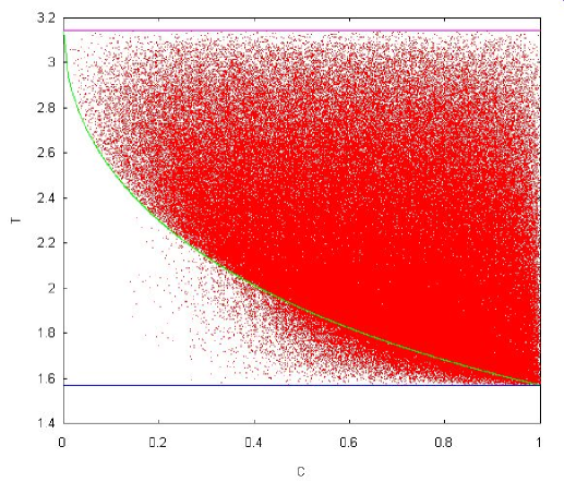
Figure 12.2: Sample of one million points representing pure states generated according to the usual Haar measure. The time $\tau$ (in units of $\hbar/\epsilon$) needed to reach its minimum overlap vs. its entanglement is shown. We also plot the $C-$ min $\tau$ curve for comparison. It is plain from this figure that most of states with minimum overlap tend to stay above the $C-$ min $\tau$ curve. See text for details.

Figure 12.3: Distributions $N(\tau)$ (not normalized) of the number of states in Fig.12.2, as a function of time $\tau$ (in units of $\hbar/\epsilon$), for different fixed amounts of entanglement. With further increase of entanglement, these distributions become more neatly peaked. See text for details.

12.2 Two entangled indistinguishable particles

Here we are going to explore the connection between entanglement and the speed of quantum evolution for systems constituted by two indistinguishable particles. In this case the concept of entanglement exhibits some extra subtleties, as compared with the case of distinguishable subsystems. When dealing with indistinguishable particles, the correlations that arise purely from the concomitant statistics (either fermionic or bosonic) do not constitute a useful resource and, consequently, must not be regarded as contributing to the amount of entanglement of the system’s state [168]. A useful formalism to describe the entanglement of systems consisting of identical particles, that takes into account the above remarks, has been advanced by Eckert et al. in [168]. For two identical bosons, the system of lowest dimensionality exhibiting the phenomenon of entanglement is a pair of bosons with a two dimensional single particle Hilbert space. The simplest fermionic system endowed with entanglement is a system of two fermions with a three dimensional single particle Hilbert space.

12.2.1 Bosons

Using the second quantization formalism, the general (pure) state of two bosons (with a two-dimensional single particle Hilbert space) can be written under the guise [168]

$$|V\rangle=\sum_{i,j=0}^{1}v_{ij}b_{i}^{\dagger}b_{j}^{\dagger}|0\rangle,$$ (12.20)

where $b_{i}^{\dagger}$ and $b_{i}$ denote bosonic creation and annihilation operators, the coefficients $v_{ij}$ constitute the symmetric matrix

$$\hat{V}=\left(\begin{array}[]{cccc}v_{00}&v_{01}\\ v_{10}&v_{11}\end{array}\right).$$ (12.21)

That is, $v_{ij}=v_{ji}$. Normalization imposes the condition $2\sum_{i,j=0}^{1}|v_{ij}|^{2}=1$.

The Hamiltonian associated with two non-interacting bosons is,

$$\hat{H}=\sum_{k=0}^{1}\epsilon_{k}b_{k}b_{k}^{\dagger},$$ (12.22)

where $b_{0}^{\dagger}|0\rangle$ is the single particle ground state with energy $\epsilon_{0}=0$, and $b_{1}^{\dagger}|0\rangle$ is the single particle excited state with energy $\epsilon_{1}=\epsilon$. The state (12.20) evolves according to the time-dependent Schrödinger equation,

$$i\hbar\frac{d}{dt}|V(t)\rangle=\hat{H}|V(t)\rangle=\sum_{i,j=0}^{1}(\epsilon_{i}+\epsilon_{j})v_{ij}(t)b_{i}^{\dagger}b_{j}^{\dagger}|0\rangle,$$ (12.23)

The general solution of this evolution equation is given by the time dependent coefficients,

$$v_{ij}(t)=v_{ij}(0)\,e^{-i\frac{(\epsilon_{i}+\epsilon_{j})}{\hbar}t}.$$ (12.24)

The time $\tau$ required to evolve into an ortonormal state is

$$\langle V(0)|V(\tau)\rangle=2\sum_{i,j=0}^{1}|v_{ij}(0)|^{2}\,e^{-i\frac{(\epsilon_{i}+\epsilon_{j})}{\hbar}\tau}=0.$$ (12.25)

Setting $z\equiv e^{-i\frac{\epsilon\tau}{\hbar}}=e^{-i\alpha}$, the orthogonality condition (12.25) can be recast as a polynomial equation in $z$, that has to admit roots of modulus equal to $1$. From this last requirement, and taking into account the symmetries in the coefficients $v_{ij}$, it follows that the coefficients can be parameterized as,

$$|v_{00}|^{2} = \Gamma$$ (12.26)

$$|v_{01}|^{2} = -\Gamma{\rm cos}\alpha$$ (12.27)

$$|v_{11}|^{2} = \Gamma,$$ (12.28)

with $\Gamma>0$ and $\alpha\in[\pi/2,3\pi/2]$. The normalization constraints also implies that $\Gamma=\frac{1}{4(1-{\rm cos}\alpha)}$. The expectation values of the energy and its square read

$$E = \langle H\rangle=2\sum_{i,j=0}^{1}|v_{ij}(0)|^{2}\,(\epsilon_{i}+\epsilon_{j})=\epsilon$$ (12.29)

$$\langle H^{2}\rangle = 2\sum_{i,j=0}^{1}|v_{ij}(0)|^{2}\,(\epsilon_{i}+\epsilon_{j})^{2}=(4\Gamma+1)\epsilon^{2},$$ (12.30)

and consequently the minimum evolution time (12.16) is

$$T_{min}=\frac{\pi\hbar}{4\epsilon\sqrt{\Gamma}}.$$ (12.31)

The formula for the concurrence in the two-boson case is [168]

$$C_{B}=4|v_{00}v_{11}-v_{01}^{2}|,$$ (12.32)

which is clearly time-independent.

For a given value of the concurrence, the minimum and maximum times for evolution to an orthogonal state can be obtained in the same way as in the case of two distinguishable qubits. The concomitant curves are exhibited in Fig.12.4.

Comparing Fig.12.4 with Fig.12.1 we see that the same general trends exhibited by a system of two distinguishable qubits are also observed in the case of two identical boson.

Figure 12.4: Curves in the $(C,\tau/T_{min})$-plane corresponding, for each value of $C$, to the states of two bosons with maximum and minimum $\tau/T_{min}$. The points represent randomly generated individual states that evolve to an orthogonal state. All depicted quantities are dimensionless.

12.2.2 Fermions

Now we are going to study a system of two identical fermions with a three dimensional single particle Hilbert space. In second quantization notation, the general (pure) state of such a system is,

$$|W\rangle=\sum_{i,j=0}^{3}w_{ij}f_{i}^{\dagger}f_{j}^{\dagger}|0\rangle,$$ (12.33)

where $f_{i}^{\dagger}$ and $f_{i}$ denote fermionic creation and annihilation operators, respectively, and the coefficients $w_{ij}$ constitute the anti-symmetric matrix

$$\hat{W}=\left(\begin{array}[]{cccc}0&w_{01}&w_{02}&w_{03}\\ w_{10}&0&w_{12}&w_{13}\\ w_{20}&w_{21}&0&w_{23}\\ w_{30}&w_{31}&w_{32}&0\end{array}\right).$$ (12.34)

That is, $w_{ij}=-w_{ji}$. Normalization imposes the condition $\sum_{i,j=0}^{3}|w_{ij}|^{2}=1/2$. The Hamiltonian describing two non-interacting particles is given by,

$$\hat{H}=\sum_{k=0}^{1}\epsilon_{k}f_{k}f_{k}^{\dagger},$$ (12.35)

and the coefficients

$$w_{ij}(t)=w_{ij}(0)\,e^{-i\frac{(\epsilon_{i}+\epsilon_{j})}{\hbar}t},$$ (12.36)

describe a general solution of the concomitant time depending Schrödinger equation. Let $z\equiv e^{-i\frac{\epsilon\tau}{\hbar}}=e^{-i\alpha}$. The evolution time to an orthogonal state follows from the condition

$$\langle W(0)|W(\tau)\rangle = 2\sum_{i,j=0}^{3}|w_{ij}(0)|^{2}\,e^{-i\frac{(\epsilon_{i}+\epsilon_{j})}{\hbar}\tau}$$ (12.37)

$$= 4z\left(|w_{01}|^{2}+|w_{02}|^{2}\,z+Mz^{2}+|w_{13}|^{2}\,z^{3}+|w_{23}|^{2}\,z^{4}\right)\,$$ (12.38)

$$= \,0,$$ (12.39)

with $M=|w_{03}|^{2}+|w_{12}|^{2}$. The polynomial equation (12.37) may have either (i) fourth real roots, (ii) two real roots and two complex (complex conjugated) roots, or (iii) two pairs of complex conjugated roots. Since we are interested in solutions of the type $e^{-i\frac{\epsilon}{\hbar}\tau}$, the most general case of interest is (iii). Consequently, the two solutions of (12.37) corresponding to (positive) times of evolution into an orthogonal state are of the form $z_{1}\equiv e^{-i\alpha}$ and $z_{2}\equiv e^{-i\beta}$. Taking into account the antisymmetric nature of $w_{ij}$, we get the following relations

$$|w_{01}|^{2} = x$$ (12.40)

$$|w_{02}|^{2} = -2\,x({\rm{cos}}\alpha+{\rm{cos}}\beta)$$ (12.41)

$$|w_{03}|^{2}+|w_{12}|^{2} = 2\,x(1+2{\rm{cos}}\alpha\,{\rm{cos}}\beta)$$ (12.42)

$$|w_{13}|^{2} = -2\,x({\rm{cos}}\alpha+{\rm{cos}}\beta)$$ (12.43)

$$|w_{23}|^{2} = x,$$ (12.44)

where the value of the parameter $x$ is determined by the normalization requirement. We want to find the fastest solution to the first orthogonal state. The time $\tau$ required to reach an orthogonal state is

$$\tau=\frac{\hbar}{\epsilon}\times min(\alpha,\beta).$$ (12.45)

Let us consider the case $\beta=\pi$. Then, the time required to arrive to an orthogonal state is equal to $\tau=\hbar\alpha/\epsilon$ and the coefficients characterizing the quantum state are,

$$|w_{01}|^{2} = \frac{1}{32\,(1-{\rm{cos}}\alpha)}$$ (12.46)

$$|w_{02}|^{2} = \frac{1}{16}$$ (12.47)

$$|w_{03}|^{2}+|w_{12}|^{2} = \frac{1-2{\rm{cos}}\alpha}{16\,(1-{\rm{cos}}\alpha)}$$ (12.48)

$$|w_{13}|^{2} = \frac{1}{16}$$ (12.49)

$$|w_{23}|^{2} = \frac{1}{32\,(1-{\rm{cos}}\alpha)},$$ (12.50)

with the obvious condition $\cos\alpha<1/2$ (that is, $\alpha\in[\pi/3,\pi]$). The energy and energy square expectation values read

$$E = \langle H\rangle=2\sum_{i,j=0}^{3}|w_{ij}(0)|^{2}\,(\epsilon_{i}+\epsilon_{j})=3\epsilon$$ (12.51)

$$\langle H^{2}\rangle = 2\sum_{i,j=0}^{3}|w_{ij}(0)|^{2}\,(\epsilon_{i}+\epsilon_{j})^{2}=\,\frac{\epsilon^{2}}{2}\left[\frac{21-19\cos\alpha}{1-\cos\alpha}\right],$$ (12.52)

and, consequently, the minimum evolution time (12.16), after some calculation, is

$$T_{min}\,=\,\frac{\pi\hbar}{2\epsilon}\,\sqrt{\frac{2(1-\cos\alpha)}{3-\cos\alpha}}.$$ (12.53)

The formula for the concurrence in the two-fermion case is [168]

$$C_{F}=8|w_{01}w_{23}-w_{02}w_{13}+w_{03}w_{12}|,$$ (12.54)

which is clearly time-independent (for the Hamiltonian (12.35)).

One can check that the lowest value of $\tau/T_{min}$ corresponds to $\cos\alpha=1/2$. That is, the state closest to saturate the lower bound for the time required to reach an orthogonal state is given by $\alpha=\pi/3$. In this case the fermionic concurrence reads

$$C_{F}=\frac{|e^{i\phi_{01}+i\phi_{23}}-e^{i\phi_{02}+i\phi_{13}}|}{2},$$ (12.55)

where $\phi_{ij}$ denotes the phase associated with the coefficient $w_{ij}$. Now, with an appropriate choice of the $\phi^{\prime}s$, we can make (12.55) either $0$ or $1$. In other words, among those states that saturate the lower bound on the time to evolve to an orthogonal state, there are states of zero entanglement, as well as maximum entangled states.

Figure 12.5: Randomly generated states of two fermions that evolve to an orthogonal state. Each point corresponds to one of those states, represented in the $(C,\tau/T_{min})$-plane. This curtain-like plot is obtained by fixing the concurrence at intervals of $0.01$. It transpires from the figure that for each value of the concurrence $C$ the time $\tau/T_{min}$ needed to reach an orthogonal state may adopt any value, from $\frac{1}{3}\sqrt{10}$ up to a maximum equal to $2$. All depicted quantities are dimensionless.

Fig.12.5 exhibits a plot in the $(C,\tau/T_{min})$-plane of a set of randomly generated states of two fermions that evolve to an orthogonal state. Each point represents one of those states. It transpires from the figure that for each value of the concurrence $C$ the time $\tau/T_{min}$ needed to reach an orthogonal state may adopt any value, from $\frac{1}{3}\sqrt{10}$ up to a maximum equal to $2$.

We see that, as far as the connection between entanglement and the “speed” of quantum evolution is concerned, the behaviour of fermionic systems differs considerably from the behaviour of systems consisting either of bosons, or of distinguishable particles.

12.3 Concluding remarks

We have explored, for bipartite systems of low dimensionality, some aspects of the connection between entanglement and the speed of quantum evolution. We considered (i) two qubits (distinguishable) systems and (ii) systems composed of two (bosonic or fermionic) identical particles, with single particle Hilbert spaces of lowest dimensionality.

These results corroborate that there is a clear correlation between the amount of entanglement and the speed of quantum evolution for systems of two-qubits and systems of two identical bosons. On the contrary, such a clear correlation is lacking in the case of systems of identical fermions [244].

Chapter 13 Evolution of entanglement in a quantum algorithm: Grover’s search algorithm

Let us revisit the algorithm introduced by Lov Grover in 1996 for a faster search in a database than any classical computer can perform (See Chapter 2 for more details). We shall pay special attention to the evolution of the entanglement present between the qubits in a given register because, as exhaustively mentioned throughout the present work, quantum entanglement is an essential ingredient for all these new revolutionary tasks. By tracing the evolution of entanglement during the search, we shall obtain a better insight into how this algorithm works.

Suppose that we have a quantum circuit with an input register of $n$ qubits plus some auxiliary ancillas, which are not of our concern now. A key ingredient in the algorithm is the Hadamard gate

$$H=\frac{1}{\sqrt{2}}\left[\matrix{1&1\cr 1&-1\cr}\right],$$ (13.1)

which converts single qubit states into a coherent superposition of them. It is convenient to introduce the gate $W$ resulting of the action of $n$ times the application of the Hadamard gate in our quantum circuit

$$W = H\otimes H\otimes...\otimes H\,(\equiv H^{\otimes n})\,|0...0\rangle\,=\,\frac{1}{\sqrt{2^{n}}}\big{(}|00...00\rangle+$$ (13.3)

$$|00...01\rangle+...+|11...11\rangle\big{)}\,=\,\frac{1}{\sqrt{2^{n}}}\sum_{i=0}^{2^{n}-1}|i\rangle$$

on the initial register of $n$ qubits, set initially at ${\bf x}=|{\bf 0}\rangle$. It is clear that what the $W$ gate does is to create a uniform superposition of all possible states of the register of $n$ qubits, starting from an initial state preparation of all states being reset to $|{\bf 0}\rangle$.

We also need an operator ($2^{n}\times 2^{n}$ matrix) that flips only the first qubit ($|0\rangle\rightarrow-|0\rangle$), while leaving the remaining $n-1$ untouched ($|{\bf x}\rangle\rightarrow|{\bf x}\rangle$). We then have the gate

$$I_{0}=\left[\matrix{-1&0&0&\cdots&0\cr 0&1&0&\cdots&0\cr 0&0&1&\cdots&0\cr\vdots&\vdots&\vdots&\ddots&\vdots\cr 0&0&0&\cdots&1\cr}\right].$$ (13.4)

Now we wonder about the composite action $G=WI_{0}W$ on an arbitrary state $\Psi=$($|a\rangle|b\rangle|c\rangle...|z\rangle$), that is, we firstly apply in our quantum circuit (13.3) to $\Psi$, followed by (13.4) and finally let us act (13.3) again. The resulting state is given by

$$\left[\matrix{(-1+\frac{2}{2^{n}})a+\frac{2}{2^{n}}(b+c+...+z)\cr\frac{2}{2^{n}}a+(-1+\frac{2}{2^{n}})b+\frac{2}{2^{n}}(c+d+...+z)\cr\vdots\cr\frac{2}{2^{n}}(a+b+...+y)+(-1+\frac{2}{2^{n}})z\cr}\right].$$ (13.5)

The outcome of $G|{\bf 0}\rangle$ has a clear significance: every element is inverted around its mean, that is, every single element value $x_{j}$ of the $n$ qubits at stage or iteration $j$, turns into a new value $x_{j+1}=2\overline{\alpha}-x_{j}$. We have to wait for the last ingredient to give sense to $G|{\bf 0}\rangle$. During our search we need a “black box” or oracle that identifies the element(s) we seek in the search. This is tantamount to assign the value $0$ to the element which does not accomplish the characteristics of the search, while to give the value $1$ to the element(s) that is(are) sought. To be more precise, every time we ask the oracle, we perform the operation

$$F({\bf x}):x\Longrightarrow(-1)^{f(x)}|x\rangle,$$ (13.6)

where $f(x)$ is either zero or one for some $k$ values out of $2^{n}$ components of the general state $|\Psi_{j}({\bf x})\rangle$, at iteration $j$, of our register of $n$ qubits .

Now we can give sense to the action $-GF$ on the register $|{\bf x}\rangle$. Suppose that there is only one element out of $n$ qubits that is being sought. The initial state preparation is such that we have the following configuration


 $\_{}$$\_{}$$\_{}$$\_{}$$\_{}$$\_{}$$\_{}$ $\_{}$$\_{}$$\_{}$$\_{}$$\_{}$$\_{}$$\_{}$$\_{}$ $\_{}$$\_{}$$\_{}$$\_{}$$\_{}$$\_{}$$\_{}$$\_{}$ $\_{}$$\_{}$$\_{}$$\_{}$$\_{}$$\_{}$$\_{}$$\_{}$ $\_{}$$\_{}$$\_{}$$\_{}$$\_{}$$\_{}$$\_{}$$\_{}$ $\_{}$$\_{}$$\_{}$$\_{}$$\_{}$$\_{}$$\_{}$$\_{}$ $\_{}$$\_{}$$\_{}$$\_{}$$\_{}$$\_{}$$\_{}$$\_{}$ $\_{}$$\_{}$$\_{}$$\_{}$$\_{}$$\_{}$$\_{}$$\_{}$ $\_{}$$\_{}$$\_{}$$\_{}$$\_{}$$\_{}$$\_{}$$\_{}$ $\_{}$$\_{}$$\_{}$$\_{}$$\_{}$$\_{}$$\_{}$$\_{}$ $\_{}$$\_{}$$\_{}$$\_{}$$\_{}$$\_{}$$\_{}$$\_{}$ $\_{}$$\_{}$$\_{}$$\_{}$$\_{}$$\_{}$$\_{}$$\_{}$ 

$c_{0}\,\,\,\,\,\,\,\,\,c_{1}\,\,\,\,\,\,\,\,\,\,\,c_{2}\,\,\,\,\,\,\,\,\,\,\,\,\,c_{3}\,\,\,\,\,\,\,\,\,\,\,\,c_{4}\,\,\,\,\,\,\,\,\,\,\,\,c_{5}\,\,\,\,\,\,\,\,\,\,\,\,\,c_{6}\,\,\,\,\,\,\,\,\,\,\,c_{7}\,\,\,\,\,\,\,\,\,\,\,\,\,c_{8}\,\,\,\,\,\,\,\,\,\,\,\,c_{9}\,\,\,\,\,\,\,\,\,\,\,c_{10}\,\,\,\,\,\,\,\,\,\,\,...\,\,\,\,\,\,\,\,c_{N-1}$

where $N=2^{n}$ and all the amplitudes are equal to $\frac{1}{\sqrt{2^{n}}}$. Suppose that the element $c_{0}$ is the one we are looking for. Let us now apply $F$ such that


$\_{}$$\_{}$$\_{}$$\_{}$$\_{}$$\_{}$$\_{}$ $\_{}$$\_{}$$\_{}$$\_{}$$\_{}$$\_{}$$\_{}$$\_{}$ $\_{}$$\_{}$$\_{}$$\_{}$$\_{}$$\_{}$$\_{}$$\_{}$ $\_{}$$\_{}$$\_{}$$\_{}$$\_{}$$\_{}$$\_{}$$\_{}$ $\_{}$$\_{}$$\_{}$$\_{}$$\_{}$$\_{}$$\_{}$$\_{}$ $\_{}$$\_{}$$\_{}$$\_{}$$\_{}$$\_{}$$\_{}$$\_{}$ $\_{}$$\_{}$$\_{}$$\_{}$$\_{}$$\_{}$$\_{}$$\_{}$ $\_{}$$\_{}$$\_{}$$\_{}$$\_{}$$\_{}$$\_{}$$\_{}$ $\_{}$$\_{}$$\_{}$$\_{}$$\_{}$$\_{}$$\_{}$$\_{}$ $\_{}$$\_{}$$\_{}$$\_{}$$\_{}$$\_{}$$\_{}$$\_{}$ $\_{}$$\_{}$$\_{}$$\_{}$$\_{}$$\_{}$$\_{}$$\_{}$ $\_{}$$\_{}$$\_{}$$\_{}$$\_{}$$\_{}$$\_{}$$\_{}$ 
 
$c_{0}\,\,\,\,\,\,\,\,\,c_{1}\,\,\,\,\,\,\,\,\,\,\,c_{2}\,\,\,\,\,\,\,\,\,\,\,\,\,c_{3}\,\,\,\,\,\,\,\,\,\,\,\,c_{4}\,\,\,\,\,\,\,\,\,\,\,\,c_{5}\,\,\,\,\,\,\,\,\,\,\,\,\,c_{6}\,\,\,\,\,\,\,\,\,\,\,c_{7}\,\,\,\,\,\,\,\,\,\,\,\,\,c_{8}\,\,\,\,\,\,\,\,\,\,\,\,c_{9}\,\,\,\,\,\,\,\,\,\,\,c_{10}\,\,\,\,\,\,\,\,\,\,\,...\,\,\,\,\,\,\,\,c_{N-1}$

$c_{0}$ is being flipped. By reversing about the mean,


 $\_{}$$\_{}$$\_{}$$\_{}$$\_{}$$\_{}$$\_{}$ $\_{}$$\_{}$$\_{}$$\_{}$$\_{}$$\_{}$$\_{}$$\_{}$ $\_{}$$\_{}$$\_{}$$\_{}$$\_{}$$\_{}$$\_{}$$\_{}$ $\_{}$$\_{}$$\_{}$$\_{}$$\_{}$$\_{}$$\_{}$$\_{}$ $\_{}$$\_{}$$\_{}$$\_{}$$\_{}$$\_{}$$\_{}$$\_{}$ $\_{}$$\_{}$$\_{}$$\_{}$$\_{}$$\_{}$$\_{}$$\_{}$ $\_{}$$\_{}$$\_{}$$\_{}$$\_{}$$\_{}$$\_{}$$\_{}$ $\_{}$$\_{}$$\_{}$$\_{}$$\_{}$$\_{}$$\_{}$$\_{}$ $\_{}$$\_{}$$\_{}$$\_{}$$\_{}$$\_{}$$\_{}$$\_{}$ $\_{}$$\_{}$$\_{}$$\_{}$$\_{}$$\_{}$$\_{}$$\_{}$ $\_{}$$\_{}$$\_{}$$\_{}$$\_{}$$\_{}$$\_{}$$\_{}$ $\_{}$$\_{}$$\_{}$$\_{}$$\_{}$$\_{}$$\_{}$$\_{}$ 

$c_{0}\,\,\,\,\,\,\,\,\,c_{1}\,\,\,\,\,\,\,\,\,\,\,c_{2}\,\,\,\,\,\,\,\,\,\,\,\,\,c_{3}\,\,\,\,\,\,\,\,\,\,\,\,c_{4}\,\,\,\,\,\,\,\,\,\,\,\,c_{5}\,\,\,\,\,\,\,\,\,\,\,\,\,c_{6}\,\,\,\,\,\,\,\,\,\,\,c_{7}\,\,\,\,\,\,\,\,\,\,\,\,\,c_{8}\,\,\,\,\,\,\,\,\,\,\,\,c_{9}\,\,\,\,\,\,\,\,\,\,\,c_{10}\,\,\,\,\,\,\,\,\,\,\,...\,\,\,\,\,\,\,\,c_{N-1}$

we obtain an enhancement of the amplitude of the element we are looking for. By repeating the action of $-GF$ several times, we arrive at the desired result with probability $p=c_{0}^{2}=1$.

How many steps do we have to do in order to find the solution? Or in other words, what is the efficiency of the algorithm? So far we have supposed that there is one only item to be found, but there can exist several of them. Suppose that according to this criterion, we represent the general state vector of the register at iteration $j$ by the wave function

$$|\Psi_{j}({\bf x})\rangle\,=\,s_{j}\sum_{{\bf x}\in S}|{\bf x}\rangle+c_{j}\sum_{{\bf x}\in NS}|{\bf x}\rangle,$$ (13.7)

where $S$ is the set of $k$ solutions of the oracle $f({\bf x})=1$ (number of items pursued), whereas there are $2^{n}-k$ terms of (13.7) which are not (set $NS$). This decomposition proves to be extremely useful. We assume without loss of generality that the coefficients in (13.7) are real. After the oracle, we have

$$|\Psi_{j}^{\prime}({\bf x})\rangle\,=\,-s_{j}\sum_{{\bf x}\in S}|{\bf x}\rangle+c_{j}\sum_{{\bf x}\in NS}|{\bf x}\rangle.$$ (13.8)

Recall that the average of amplitudes of (13.8) at this stage is given by

$$\overline{\alpha}\,=\,\frac{1}{2^{n}}\big{(}-s_{j}k+c_{j}(2^{n}-k)\big{)}.$$ (13.9)

After application of operator $-GF$, we get the new state ($j+1$)

$$|\Psi_{j+1}({\bf x})\rangle\,=\,s_{j+1}\sum_{{\bf x}\in S}|{\bf x}\rangle+c_{j+1}\sum_{{\bf x}\in NS}|{\bf x}\rangle,$$ (13.10)

where we have the celebrated “inversion around the mean” expressions $s_{j+1}=2\overline{\alpha}-s_{j},\,c_{j+1}=2\overline{\alpha}-c_{j}$. Expanding coefficients we have two recursion relations between coeficients $s_{j+1}$ and $c_{j+1}$, that transforms ($s_{j},c_{j}$) into ($s_{j+1},c_{j+1}$) (the action of $-GF$). Because all operations done on the generic state $|\Psi_{j}({\bf x})\rangle$ are unitary, due to the fact that it is initially normalized to unity ($s_{0}=c_{0}=\frac{1}{\sqrt{2^{n}}}$), it must preserve its norm. This condition entails that

$$|\langle\Psi_{j}({\bf x})|\Psi_{j}({\bf x})\rangle|^{2}\,=\,k\,s_{j}^{2}\,+\,(2^{n}-k)c_{j}^{2}\,=\,1,$$ (13.11)

which is equivalent to an ellipse with coordinates $s_{j}=\frac{1}{\sqrt{k}}\sin\theta_{j}$, $c_{j}=\frac{1}{\sqrt{2^{n}-k}}\cos\theta_{j}$, for some angle $\theta_{j}$. After simplifying the aforementioned recursion relation, we obtain

$$\sin\theta_{j+1} = \sin(\theta_{j}+\omega),$$ (13.12)

$$\cos\theta_{j+1} = \cos(\theta_{j}+\omega),$$ (13.13)

provided we identify $\cos\omega$ with $1-\frac{2k}{2^{n}}$. After imposing the initial conditions mentioned before, we arrive at the final expression for the $2^{n}$ coefficients of $|\Psi_{j}({\bf x})\rangle$ at step $j$:

$$s_{j} = \frac{1}{\sqrt{k}}\sin\big{(}(2j+1)\nu\big{)},$$ (13.14)

$$c_{j} = \frac{1}{\sqrt{2^{n}-k}}\cos\big{(}(2j+1)\nu\big{)},$$ (13.15)

with $\sin^{2}\nu=\frac{k}{2^{n}}$.

Now we are in a position to answer the previous question. We have finished the search once we have absolute certainty about the result. In other words, $ks_{j}^{2}=\sin^{2}\big{(}(2j+1)\nu\big{)}=1$ for some $j^{*}$. If the number of qubits $n$ is high enough, then $j^{*}$ is the closest integer value to

$$\bigg{[}\frac{\pi}{4}\sqrt{\frac{2^{n}}{k}}\bigg{]}\,=\,O(\sqrt{2^{n}}).$$ (13.16)

With this analysis we show that Grover’s algorithm is of $O(\sqrt{N})$, as opposed to the best classical result $N/2$.

Where is entanglement in all this business? Whenever we apply $-GF$ on a reference state, we induce all qubits to interact between them. If we start with the state ${\bf x}=|{\bf 0}\rangle$ at zero iterations, we do not have any entanglement initially. But as soon as we make them interact, we create several superpositions of all possible states of the register, until a single state is reached, the solution to the search algorithm. Therefore we end up in a product state and no entanglement is present.

Let us consider the measure of entanglement introduced in previous Chapters. It is based on the conjecture (numerically checked by us) that the inequality [154]

$$0\,\leq\,d_{E}\equiv C^{2}_{1(2..n)}-\sum_{i=2}^{n}C^{2}_{1i}\,\leq\,1$$ (13.17)

holds for an arbitrary number $n$ of qubits in a pure state $\rho=|\Psi\rangle_{1..n}\langle\Psi|$. $C^{2}_{xy}$ stands for the concurrence squared between qubits $x,y$ and $C^{2}_{1(2..n)}=4\,$det$\rho_{1}$, with $\rho_{1}$=Tr_2..n($\rho$). We regard the quantity $d_{E}$ between inequalities as a proper measure for multipartite entanglement, an so it is considered here.

Figure 13.1: Evolution for a 6-qubit register of the target amplitude or probability (curve reaching 1), and the amplitude or probability of the remaining non-target qubits (lowest curve), in absolute value. The curve with two maximums plots the evolution of 13.17 during a whole period. See text for details.

Suppose the we have a quantum computer with a definite number of qubits upon which we want to apply our Grover’s search algorithm. In Fig.13.1 we plot the evolution for a system with $n=6$ qubits of the absolute values of the amplitudes for the “target” state (curve reaching 1) and all the remaining amplitudes (curve reaching 0) versus the number of iterations $j$. The periodic evolution described by (13.14) is apparent. Even when we have already found the solution (amplitude equal to one), we obtain it again and again. From inspection, we see that the critical value at which the solution is reached is $j_{c}=6$, which coincides with the predicted value $j^{*}(k=1)$ (13.16). The evolution of entanglement $d_{E}$ is described by the curve in between. It is remarkable that the maximum value is obtained at exactly $j_{c}/2$ iterations, being null again when the solution is found. Fig.13.2 depicts the same quantities for $n=10$ qubits. In this plot the shape of a sinus or a cosinus for the amplitudes is more precise. Again we observe a periodical evolution for $d_{E}$, but there appears an interesting feature. Once the solution has been reached at $j=j_{c}$, there is a revival at $3j_{c}/2$ in the entanglement which is greater that in the way to pursue the result at $j=j_{c}/2$. We do not quite understand the meaning of this feature, but there is no reason that prevents this fact.

Figure 13.2: Same as in Fig. 13.1, for a 10-qubit register. The perfect harmonic evolution of the amplitudes becomes apparent as the number of qubits increases. See text for details.

This example of quantum algorithm improves the speed of calculation by a factor of $O(\sqrt{N})$ with respect to the best classical result. Some may say that this is not the spectacular exponential result that computer scientists (induced by physicists) promised with the quantum computer business. Well, indeed it is a substantial improvement even nowadays. Let us see why.

Whenever we make a search in the internet, for instance we are looking for “Perico de los Palotes Bush”, there usually appears the result within few seconds or fractions of seconds. Notwithstanding the fact that it is certainly a useful achievement, it cannot be used against an eventual quantum computer. The tricky thing is that the searches are performed in a database arranged alphabetically, and it automatically updates during the night. So it is not the kind of problem of searching for a needle in a haystack like the one we are dealing with here. It resembles more the situation of finding a given number in the phone book. In point of fact, the algorithm we use in the real life is similar to a bisection method: we take half of the book, then one of the quarters, and so forth until we find the desired item. We could say that convergence is exponential. But what if we are given the telephone number and look for the owner? Suppose that we live in the Balearic Islands and it is high season for tourism . Suppose that there is a population of one million inhabitants. If they were registered at random, to find someone would take of the order of 500000 steps minimum, while around 1000 using a quantum computer and the Grover’s algorithm (only 10 qubits needed). Certainly not an exponential improvement, but considerable. The paradigm of exponential speed-up is the Shor algorithm for factorizing large numbers which owes, in turn, much of its efficiency to the algorithm that performs the Quantum Fourier Transform (QFT) (see Chapter 2 for more details). Although it is a bit more complex than Grover’s, the QFT algorithm relies also on registers of qubits that are collectively entangled during the different iterations that take place. If we had followed its study along the same line as Grover’s, we would had seen that entanglement constitutes indeed an essential ingredient.

Summing up, two physical mechanisms make possible the astonishing predicted achievements of quantum computing: on the one hand quantum entanglement, a purely quantum correlation, and on the other hand quantum parallelism, the superposition principle.

Chapter 14 Entanglement and quantum phase transitions

In Chapter 5 the concept of Generalized Entanglement and the $h$-purity measure [146] were introduced, a generalization which goes beyond the usual notion [158], where a subsystem decomposition exists, and which is relative to a preferred set of observables. In this definition a pure quantum state is Generalized Unentangled (Generalized Entangled) if it induces a pure (mixed) reduced state on that set of observables.

A measure of Generalized Entanglement is the relative purity or $h$-purity, where $h=\{O_{j}\}$ is an orthogonal and finite set of observables. The $h$-purity of a pure quantum state $|{\psi}\rangle$ is defined as

$$P_{h}={\sf K}\sum_{j}|\langle\psi|O_{j}|{\psi}\rangle|^{2}$$ (14.1)

where ${\sf K}$ is a normalization factor chosen such that the maximum relative purity is 1. In the cases analyzed in this work, a quantum state will be generalized unentangled (GU) with respect to the set $h$, whenever its $h$-purity is maximum and generalized entangled (GE) otherwise ([245]).

Nice properties are obtained whenever the set $h$ is a simple Lie Algebra. In this case, the GU states are the Generalized Coherent States (GCS) of $h$, obtained by applying a group operation to some reference state, i.e., $|{\sf GCS}\rangle=\exp[i\sum c_{j}O_{j}]|{\sf vac}\rangle$ ($c_{j}\in\mathcal{C}$). Also, the relative purity is group-invariant.

The traditional notion of entanglement is recovered when choosing the preferred set of observables $h$ as the set of all local observables, corresponding to a particular subsystem decomposition ([245]). For example, if the system studied consists of $N$-spin 1/2 particles, a measure of the usual (traditional) entanglement is obtained when calculating the purity relative to the set

$$h=\{\sigma_{x}^{1},\sigma_{y}^{1},\sigma_{z}^{1},\cdots,\sigma_{x}^{N},\sigma_{y}^{N},\sigma_{z}^{N}\},$$ (14.2)

with $\sigma_{\alpha}^{j}$ the Pauli spin-1/2 operators; that is,

$$P_{h}=\frac{1}{N}\sum\limits_{\alpha,j}|\langle\psi|\sigma_{\alpha}^{j}|{\psi}\rangle|^{2},$$ (14.3)

which reaches its maximum value ($P_{h}=1$) only for a product state of the form $|{\psi}\rangle=|{\phi_{1}}\rangle_{1}\otimes\cdots\otimes|{\phi_{N}}\rangle_{N}$. These states are the GCSs of $h$. The purity is then invariant under local rotations, which are the group operations in this case.

Although the usual notion of entanglement is easily recovered in this framework, here we analyze the generalized entanglement relative to sets of observables other than the local ones, in order to capture the most important quantum correlations that describe the physics of the models studied.

The main purpose of this Chapter is to relate quantum phase transitions and entanglement. But let us first remember the basics of a phase transition occurring at finite temperatures ($T\neq 0$). Either if we are dealing with classical or quantum systems, they are equally described by Landau’s theory [246], being the protagonist some broken symmetry of the system and some corresponding order parameter. The idea is the following: given a Hamiltonian $H$ describing a physical system, we may assume $H$ to be invariant under a certain symmetry operation. However, the ground state of that system need not preserve that very same symmetry. We say then, in this case, that the system undergoes a spontaneous symmetry breakdown. Let us illustrate it with the Heisenberg Hamiltonian

$$H=-J\sum_{(i,j)}{\bf S_{i}}\cdot{\bf S_{j}}+{\bf h}\cdot\sum_{i}{\bf S_{i}},$$ (14.4)

of $N$ spins and interaction mediated only through nearest-neighbours, with ${\bf h}$ being an external magnetic field. We recall that the average magnetisation per spin reads

$${\bf m}\equiv\frac{1}{N}\sum_{i}\langle{\bf S_{i}}\rangle.$$ (14.5)

In the limit ${\bf h}\rightarrow 0$, (14.4) is still invariant under $SO(3)$ rotations of all spins, but ${\bf m}$ does not vanish, and consequently does not observe the $SO(3)$ symmetry. We then say that there appears an spontaneous magnetisation, with a critical (maximum) temperature such that ${\bf m}\neq 0$. It is said that the vector ${\bf m}$ plays the role of an order parameter, that describes a phase transition between an ordered state (${\bf m}\neq 0$) and a disordered state (${\bf m}=0$). As we have seen, this mechanism is driven by the temperature: at low temperature, the term $TS$ in the free energy $F=\langle H\rangle-TS$ ($S$ being the entropy) may be negligible, so that minimum $F$ is equivalent to minimum $\langle H\rangle$, which happens when all spins are aligned in the same direction (ordered phase). As we increase the temperature, $TS$ dominates in $F$ and minimizing the free energy $F$ is tantamount as maximizing the entropy $S$, which is attained when all spins point at random (disordered phase).

With this example, we illustrate the tenets of Landau’s theory of phase transitions. Now then, what is the mechanism of a phase transition that occurs at zero temperature? Could the ground state energy of the system at $T=0$ be the equivalent of the previous free energy $F$? Let us consider a Hamiltonian $H(g)$ in the context of condensed matter, whose degrees of freedom reside on the sites of a lattice. Let us further follow the evolution of the ground state energy of $H(g)$ as a function of the parameter $g$. One possibility is that the ground state is a smooth function of $g$. On the other hand, $g$ can couple to a conserved quantity: $H(g)=H_{0}+gH_{1},[H_{0},H_{1}]=0$. Therefore we can diagonalize both $H_{0}$ and $H_{1}$ at the same time so that the eigenfunctions are independent of $g$ even if the eigenvalues vary with $g$. This situation implies that whenever there is a level crossing at some $g=g_{c}$, where an excited state becomes the ground state, we come across with a point of nonanalyticity in the ground state. However, even if there is no level-crossing, it can become sharper and sharper as we increase the number of sites. In the general case, we shall identify any point of non-analytic behaviour of the ground state energy as a quantum phase transition (QPT). We do not enter too much into all the details of a QPT. The reader is referred to [249] for a comprehensive insight. Roughly speaking, the usual terminology employed in classical phase transitions (critical exponents, characteristic lengths, ..) also applies at zero temperature, where the basic difference is that transitions are induced by the change of a set of parameters $\{g_{i}\}$ of a given Hamiltonian. Even in this case, there exists two types of quantum phase transitions, namely, i) those that occur strictly a $T=0$, and ii) the ones that can take place at very low temperatures, remaining close enough to the critical point(s). In this Chapter we focus our interest in the former ones.

Summarizing, quantum phase transitions (QPTs) are qualitative changes occurring in the properties of the ground state of a many-body system due to modifications either in the interactions among its constituents or in their interactions with an external probe [249], while the system remains at zero temperature. As explained, such changes occur as some parameter $g$ of a set $\{g_{i}\}$ of a given Hamiltonian vary across some critical point or manifold. It is plain from the nature of the QPTs that thermal fluctuations do not play a relevant role, as they do in the usual phase transitions. Instead, there appear fluctuations in the expectation value of some observable, implying that QPTs are purely quantum phenomena. Examples of QPTs are provided in [249], being a paradigm the quantum paramagnet to ferromagnet transition occurring in Ising spin systems under an external transverse magnetic field [250, 251].

How do all these features relate to quantum entanglement? How does entanglement fit in the context of condensed matter physics? Entanglement is a property inherent to quantum states, which lies at the core of generic “truly” quantum correlations, as Schrödinger first pointed out [2]. These correlations arise when particles interact, leaving the system in a state that has to be described as a whole, regardless of its subsystems. In view of this definition, one would expect some considerable change in the ground state of a given system as it undergoes a quantum phase transition. In other words, one could regard the entanglement present in a quantum system as a detectable property, on equal footing as several thermodynamic variables. Specifically, a quantum phase transition offers a unique framework where to study the intimate connection between entanglement and a physical system in the thermodynamic limit $N\rightarrow\infty$.

The first steps made towards this connections have focused on characterizing entanglement using information-theoretic concepts, such as the entropy of entanglement [157], the concurrence [158], and other measures of entanglement, originally developed for bipartite systems. The arena for these studies has been those exactly solvable models that can support a quantum phase transition [147, 252, 253, 254, 255, 256]. These efforts have employed for instance the concurrence between neighbours, nearest-neighbours and so forh in the $XY$ model in a transverse magnetic field [252, 253], or have borrowed tools from renormalization group theory in the study of the entanglement between a block of nearby spins and the rest of the chain [255]. These studies certainly constitute important contributions towards the study of entanglement and criticality (universality classes, critical exponents,..) in quantum systems, but one may agree with the that fact it is a limitation to use solely bipartite entanglement measures in this enterprise. It therefore seems plausible to employ a measure of entanglement that is capable of grasping the features of all constituents in a quantum systems at once, specially in the thermodynamic limit $N\rightarrow\infty$. Here is the point where the generalized entanglement (the purity measure) introduced in Chapter 5, and at the beginning of the present one, makes its appearance. It constitutes an extension of the essential properties of entanglement beyond the conventional subsystem-based framework. References [146, 147] provide a thorough account of it, and [245] makes explicit use of the purity measure in the context of QPTs. In the latter context, the most critical step is to determine which subset of observables may be relevant in each system under study, since the $h$-purity must contain information about the quantum correlations that play a dominant role in the quantum phase transition (QPT). In particular, if the ground state of the models we consider can be exactly calculated then the relevant quantum correlations in the different phases are well understood, therefore choosing this subset of observables becomes relatively easy. This will be the case in this Chapter for the $XY$ model, and the $XY$ model with bond alternation. In a more general case where the ground state of the system cannot be exactly computed, the application of these concepts can be done in principle by following the same strategy (see Ref. [245] for a comprehensive account of these features).

As discussed in [146, 147], the purity measures recovers the properties of bipartite (as well as multipartite) entanglement measures, which are of common use in quantum information processing (QIP). However, we do not pretend to discuss its utility in those areas of QIP where measures such as the concurrence or the entropy of entanglement suffices to explain the corresponding features described. It is not the intention of this Chapter to confront different positions regarding the nature of the measure of entanglement or its relativity, as explained in Chapter 5. The aim of the present Chapter is to expand the analysis initiated in [146, 147, 245] by focusing on the detection of QPTs due to a broken symmetry. The behaviour of an appropriate relative purity of the ground state will prove its utility not only in detecting a QPT (in the cases of the $XY$ model, and the $XY$ model with bond alternation), but will also unfold several non-ergodic features in the dynamic evolution of a system during a QPT.

14.1 Static case

In this section we study the connection between quantum phase transitions (QPTs) and the concept of Generalized Entanglement, with no dynamics involved. In order to illustrate this feature, we could use the anisotropic $XY$ model, already employed in the work of the Los Alamos group ([245]). However, it is more instructive to provide an additional example with a slightly modified model, namely, the anisotropic $XY$ model with bond alternation in a transverse magnetic field. Besides, we first provide here, to our knowledge, the analytical solution of this model. In any case, the original anisotropic $XY$ model is revisited in full detail in the section devoted to the dynamic case. For an account on QPTs and systems of spins the reader is referred to [257].

With these examples, we claim to use the purity measure as a detector of a quantum phase transition in the condensed matter framework.

14.1.1 The anisotropic $XY$ model with bond alternation

In this section we study the quantum phase transitions (QPTs) of the anisotropic $XY$ model with bond alternation. The corresponding model Hamiltonian is

$$H=-g\sum\limits_{j=1}^{N}(1+(-1)^{j}\delta)\left[(1+\gamma)\sigma_{x}^{j}\sigma_{x}^{j+1}+(1-\gamma)\sigma_{y}^{j}\sigma_{y}^{j+1}\right]+\sum\limits_{j=1}^{N}\sigma_{z}^{j},$$ (14.6)

where $g$ is the coupling constant, $\gamma$ the anisotropy, and $\delta$ is the bond-alternation constant. Making $\delta=0$ in (14.6), we recover the usual anisotropic $XY$ model with transverse magnetic field. As usual, periodic boundary conditions are considered ($\sigma_{\alpha}^{j}\equiv\sigma_{\alpha}^{j+N}$). This model was first studied in [258] without including a transverse field. A similar model is studied in [259] at finite temperatures. In the present effort we also consider the action of a transverse uniform magnetic field, which modifies the concomitant ground state. To our knowledge, this is the first time that the QPTs associated to Hamiltonian (14.6) are studied in an analytic fashion.

The ground state of system (14.6) can be exactly obtained by mapping the spin 1/2 Pauli operators into the fermionic algebra in the following way:

$$a^{\dagger}_{2j-1} = \prod\limits_{k=1}^{2j-2}(-\sigma_{z}^{k})\sigma^{+}_{2j-1}$$ (14.7)

$$b^{\dagger}_{2j} = \prod\limits_{k=1}^{2j-1}(-\sigma_{z}^{k})\sigma^{+}_{2j},$$ (14.8)

where $a^{\dagger}_{2j-1}$ and $b^{\dagger}_{2j}$ are the fermionic operators that create a spinless fermion at site $2j-1$ (odd) and $2j$ (even), respectively. Here, $j=1..M=\frac{N}{2}$ and $\sigma^{+}_{l}=\frac{\sigma_{x}^{l}+i\sigma_{y}^{l}}{2}$. Defining the fermionic operators

$$a^{\dagger}_{k} = \frac{1}{\sqrt{M}}\sum\limits_{j=1}^{M}e^{ik(2j-1)}a^{\dagger}_{2j-1}$$ (14.9)

$$b^{\dagger}_{k} = \frac{1}{\sqrt{M}}\sum_{j=1}^{M}e^{ik2j}b^{\dagger}_{2j}$$ (14.10)

with $k=l\frac{2\pi}{N}$, and $l=1\cdots M$, the Hamiltonian of Eq. 14.6 can be rewritten as $H=\sum_{k\in W}H_{k}$, with $W=\{\frac{2\pi}{N},\frac{4\pi}{N},\cdots,\frac{\pi}{2}\}$, and

$$H_{k} = J_{k}a^{\dagger}_{k}b_{k}+J^{*}_{k}a^{\dagger}_{-k}b_{-k}+\Gamma_{k}a^{\dagger}_{k}b^{\dagger}_{-k}+\Gamma^{*}_{k}a^{\dagger}_{-k}b^{\dagger}_{k}+2(a^{\dagger}_{k}a_{k}+b^{\dagger}_{k}b_{k})+h.c.,$$ (14.11)

$$J_{k} = -4g(\cos k-i\delta\sin k),$$ (14.12)

$$\Gamma_{k} = -4g\gamma(-\delta\cos k+i\sin k).$$ (14.13)

Defining the vector operators

$$\hat{A}_{k}=\pmatrix{a_{k}\cr a^{\dagger}_{-k}\cr b_{k}\cr b^{\dagger}_{-k}},$$ (14.14)

and $\hat{A}^{\dagger}_{k}=(\hat{A}_{k})^{\dagger}$, we obtain

$$H_{k}=\hat{A}^{\dagger}_{k}\hat{H}_{k}\hat{A}_{k},$$ (14.15)

with $\hat{H}_{k}$ being the Hermitian matrix

$$\hat{H}_{k}=\pmatrix{2&0&J_{k}&\Gamma_{k}\cr 0&-2&-\Gamma_{k}&-J_{k}\cr J^{*}_{k}&-\Gamma^{*}_{k}&2&0\cr\Gamma^{*}_{k}&-J^{*}_{k}&0&-2}.$$ (14.16)

Therefore, the problem reduces to the diagonalization of the matrices $\hat{H}_{k}$ for each $k\in W$. The difference with the results obtained in [258] is that the terms in (14.16) contain the interaction with an external magnetic field, which induces as we shall see a richer structure in the concomitant phase diagram. In this way, it can be proved that the ground state energy in the thermodynamic limit is given by (up to an irrelevant global constant)

$$E_{g}=\frac{1}{2\pi}\int_{0}^{\pi/2}dk\left[\lambda_{1}(k)+\lambda_{2}(k)\right],$$ (14.17)

with

$$\lambda_{1}(k)=-\sqrt{4-\xi_{k}+16g^{2}((1+\gamma^{2}\delta^{2})\cos^{2}k+(\gamma^{2}+\delta^{2})\sin^{2}k)}$$ (14.18)

$$\lambda_{2}(k)=-\sqrt{4+\xi_{k}+16g^{2}((1+\gamma^{2}\delta^{2})\cos^{2}k+(\gamma^{2}+\delta^{2})\sin^{2}k)},$$ (14.19)

and $\xi_{k}=2\sqrt{16g^{2}(2+(2+16g^{2}\gamma^{2})\delta^{2}-2(-1+\delta^{2})\cos 2k)}$. Obviously, $\lambda_{1}(k)$ and $\lambda_{2}(k)$ are the negative eigenvalues of the matrices $\hat{H}_{k}$. Alternatively, we can diagonalize the matrix ${H}_{k}$ spanned by the eigenvectors

$${\cal D} = \{|0\rangle,a_{k}^{\dagger}a_{-k}^{\dagger}|0\rangle,b_{k}^{\dagger}b_{-k}^{\dagger}|0\rangle,a_{k}^{\dagger}b_{k}^{\dagger}|0\rangle,a_{k}^{\dagger}b_{-k}^{\dagger}|0\rangle,a_{-k}^{\dagger}b_{k}^{\dagger}|0\rangle,$$ (14.21)

$$a_{-k}^{\dagger}b_{-k}^{\dagger}|0\rangle,a_{k}^{\dagger}a_{-k}^{\dagger}b_{k}^{\dagger}b_{-k}^{\dagger}|0\rangle\}$$

which is an $8\times 8$ matrix, whose negative eigenvalues obviously coincide with the previous $\lambda_{1}(k),\lambda_{2}(k)$. Once we have found the eigenvalues, we find the concomitant ground state $|\Psi\rangle=\prod_{k>0}^{\pi/2}|\Psi_{k}\rangle$, with $|\Psi_{k}\rangle=u_{1}\,|0\rangle+u_{1}\,a_{k}^{\dagger}a_{-k}^{\dagger}|0\rangle+...+u_{8}\,a_{k}^{\dagger}a_{-k}^{\dagger}b_{k}^{\dagger}b_{-k}^{\dagger}|0\rangle$, in terms of the coefficients $\{u_{i}\}$. The ground state will be coherent with respect to $so(2N)$, and therefore generalized unentangled with respect to this algebra. As we saw, this is tantamount as possessing purity $P_{so(2N)}=1$, which is of no interest. Depending on the subset of observables chosen, the $h$-purity contains information about different $n$-body correlations present in the quantum state, allowing for a more general and complete characterization of entanglement.

Instead, if we consider the $u(N)$ algebra, we have a non-trival structure. We need $N^{2}$ operators, which are found to be in the basis (14.21):

$$\sqrt{2}(a_{k}^{\dagger}a_{k}-\frac{1}{2})$$ (14.22)

$$\sqrt{2}(b_{k}^{\dagger}b_{k}-\frac{1}{2})$$ (14.23)

$$(a_{k}^{\dagger}a_{k^{\prime}}+a_{k^{\prime}}^{\dagger}a_{k})\,\,\,k\neq k^{\prime}$$ (14.24)

$$i(a_{k}^{\dagger}a_{k^{\prime}}-a_{k^{\prime}}^{\dagger}a_{k})\,k\neq k^{\prime}$$ (14.25)

$$(b_{k}^{\dagger}b_{k^{\prime}}+b_{k^{\prime}}^{\dagger}b_{k})\,\,\,k\neq k^{\prime}$$ (14.26)

$$i(b_{k}^{\dagger}b_{k^{\prime}}-b_{k^{\prime}}^{\dagger}b_{k})\,k\neq k^{\prime}$$ (14.27)

$$(a_{k}^{\dagger}b_{k^{\prime}}+b_{k^{\prime}}^{\dagger}a_{k})\,\,\,\forall\,k,k^{\prime}$$ (14.28)

$$i(a_{k}^{\dagger}b_{k^{\prime}}-b_{k^{\prime}}^{\dagger}a_{k})\,\forall\,k,k^{\prime},$$ (14.29)

with $-\frac{\pi}{2}<k<\frac{\pi}{2}$. If we are eager to obtain the purity $P_{u(N)}$ in the ground state, we take advantage of the symmetries of Hamiltonian (14.11) ($H_{k}$ mixes $k$ with $-k$). This means that few operators of the set (14.22) will survive in the computation of $P_{u(N)}$. Therefore, what remains is

$$P_{u(N)} = \frac{2}{N}\sum_{k>0}^{\pi/2}\bigg{(}2[\langle a_{k}^{\dagger}a_{k}-\frac{1}{2}\rangle^{2}+\langle a_{-k}^{\dagger}a_{-k}-\frac{1}{2}\rangle^{2}+\langle b_{k}^{\dagger}b_{k}-\frac{1}{2}\rangle^{2}+$$ (14.33)

$$\langle b_{-k}^{\dagger}b_{-k}-\frac{1}{2}\rangle^{2}]+4|\langle a_{k}^{\dagger}a_{-k}\rangle|^{2}+4|\langle b_{k}^{\dagger}b_{-k}\rangle|^{2}+$$

$$4|\langle a_{k}^{\dagger}b_{k}\rangle|^{2}+4|\langle a_{k}^{\dagger}b_{-k}\rangle|^{2}+4|\langle a_{-k}^{\dagger}b_{k}\rangle|^{2}+$$

$$4|\langle a_{-k}^{\dagger}b_{-k}\rangle|^{2}\bigg{)}.$$

The expectation values are obtained in terms of coefficients $\{u_{i}\}$ of the ground state (for instance, $\langle a_{k}^{\dagger}a_{k}\rangle=|u_{2}|^{2}+|u_{4}|^{2}+|u_{5}|^{2}+|u_{8}|^{2}$). The numerical computation of the purity $P_{u(N)}$ as $N\rightarrow\infty$ is then carried out. In the case of no bond alternation ($\delta=0$) one recovers the study performed in [245]. It is shown there that the corresponding $u(N)$ purity $P_{u(N)}$ reads

$$P_{u(N)}=\left\{\begin{array}[]{cl}\frac{1}{1-\gamma^{2}}\bigg{(}1\,-\,\frac{\gamma^{2}}{\sqrt{1-4g^{2}(1-\gamma^{2})}}\bigg{)}&\mbox{ if }g\leq\frac{1}{2}\cr\frac{1}{1+\gamma}&\mbox{ if }g>\frac{1}{2}\end{array}\right.\;.$$ (14.34)

Eq. (14.33) reduces to (14.34) for $\delta=0$, which presents an analytical expression. In forthcoming sections we shall study the dynamic properties of the $XY$ model with no bond alternation, and eventually compare those features with the concomitant static case, whose purity is given by (14.34).

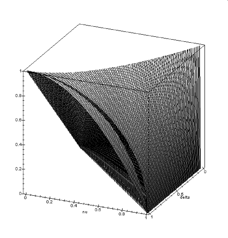
Figure 14.1: Phase diagram of Hamiltonian (14.6) representing $\gamma^{(I)}$ and $\gamma^{(II)}$ in (14.35) vs. the bond alternating parameter $\delta$ and $\nu\equiv\frac{h}{2g}$ (see text). On the one hand, as we decrease the transverse magnetic field $h$ ($\nu\rightarrow 0$) in (14.6), the system presents a bond-order, so the surface collapses to the line $\gamma=\delta$, agreeing with the results in Ref. [258]. On the other hand, by reducing the bond alternating parameter $\delta$, the surface reduces to the vertical line $\nu=1$, which is the critical point of the usual anisotropic $XY$ model with transverse magnetic field. It is apparent from this figure that the addition of a bond alternating component to the latter model induces a very rich structure in the phase diagram. See text for details.

The ground state of this bond alternating system undergoes several QPTs while changing the coupling constants $g$ and $\delta$. The quantum phases can be studied by taking different limits in Eq. 14.6. For example, if $g<0$, $\gamma=1$, and $\delta=0$, there is no bond alternation and the model transforms into the antiferromagnetic Ising model in a transverse magnetic field. Here, the ground state undergoes an antiferromagnetic-to paramagnetic second order QPT at the critical point $g_{c}=-1/2$ (analogous to the ferromagnetic case). In fact, when $g\rightarrow-\infty$, the ground state of the system is twofold degenerate, i.e., $|{G}\rangle=2^{-1/2}\left[|{+-\cdots+-}\rangle\pm|{-+\cdots-+}\rangle\right]$, with $|{+}\rangle=2^{-1/2}(|{\uparrow}\rangle+|{\downarrow}\rangle)$ and $|{-}\rangle=2^{-1/2}(|{\uparrow}\rangle-|{\downarrow}\rangle)$ the eigenvectors of the $\sigma_{x}$ operators, while when $g\rightarrow 0$ the spins align with the external magnetic field, i.e., $|{G}\rangle=|{\downarrow\downarrow\cdots\downarrow}\rangle$.

The limit $g\rightarrow-\infty$, with $1>(\gamma,\delta)>0$ has been studied in Ref. [258]. Here, the external magnetic field is irrelevant. As mentioned above, when $\delta\rightarrow 0$ and $\gamma\rightarrow 1$ the phase is antiferromagnetic, while for $\delta\rightarrow 1$ (i.e., Eq. 14.6 becomes a sum of isolated two-spin interactions) a bond-order develops. In particular, it has been proved ([258]) that an antiferromagnetic-to-bond-order second order QPT occurs at the critical line $\delta=\gamma$, in this limit.

The phase diagram of the Hamiltonian (14.6) is, after some algebra, defined by the regions

$$\gamma^{(I)}\, = \,\sqrt{\delta^{2}-\nu^{2}}$$ (14.35)

$$\gamma^{(II)}\, = \,\frac{\sqrt{1-\nu^{2}}}{\delta}$$ (14.36)

in the $\gamma,\delta$ and $\nu\equiv\frac{h}{2g}$ space of critical parameters ($h$ being the transverse magnetic field set to 1). The critical points can be obtained either numerically by finding the zeros $(g_{c},\gamma_{c},\delta_{c})$ of the functions $\lambda_{1}(k)$ or $\lambda_{2}(k)$, or analytically. In this way, we assure that the second derivatives of the ground state energy with respect to these parameters diverge or present a discontinuity. In Fig.14.1 we plot the regions of the phase diagram defined by (14.35). Also, in [260] we show the phase-diagram for this model in the antiferromagnetic region ($g<0$), which agrees with the above description for different limits. One observes [260] that for small values of $g$ (high values of $\nu$) the phase is paramagnetic, therefore the purity in Fig.14.2 tends to one, and as we decrease $g$ (increase $\nu$) the phase becomes first antiferromagnetic (Néel order), and then it presents a bond-order. For small values of $\delta$ the antiferromagnetic region is dominant but it dissapears when $\delta\rightarrow 1$. Moreover, when $g\rightarrow-\infty$ ($\nu\rightarrow 0$) the critical line separating the antiferromagnetic and bond-order phases is located at $\gamma=\delta$, agreeing with the results in Ref. [258]. As seen from Fig.14.1, the phase diagram indeed reduces to the line $\gamma=\delta$. Also, at zero anisotropy $\gamma=0$ we encounter a new critical line at $\nu=\delta$, which results from the competition of the bond alternating order between spins and their alignment with the external magnetic field $h$.

These analytic results are in excellent agreement with the numerical results computing the points where the derivative of the purity $P_{u(N)}$ (with respect to any element of the parameter space) diverge. This fact validates all our previous calculations regarding the features relative to the purity as a detector of a QPT.

Figure 14.2: Evolution of the purity measure $P_{u(N)}$ (solid line) as a function of the parameter $\nu\equiv\frac{h}{2g}$ for the bond alternating system (14.6). Its derivative (dashed lines) “detects” the presence of critical points in phase space given by (14.35), which for the case of $\delta=0.9,\gamma=0.8$ and $g=1$ are given by $\nu=0.412$ (region (I) in (14.35)) and $\nu=0.693$ (region (II) in (14.35)). For this set of parameters, an antiferromagnetic phase developes from $\nu=0$ to $\nu=0.412$, a bond order one from $\nu=0.412$ to $\nu=0.693$, and a final paramagnetic phase with further $\nu$-grow.

One way to check the validity of (14.35) is to trace the evolution of the purity $P_{u(N)}$ as a function of $\nu\equiv\frac{h}{2g}$. This is done in Fig.14.2. Let us consider the $g=1$ (Ising case) throughout the following discussion. The solid line depicts the purity that corresponds to $\delta=0.9,\gamma=0.8$, while the dashed one plots its derivative $\frac{dP_{u(N)}}{d\nu}$. As $\nu\equiv\frac{h}{2g}\rightarrow 0$, which means zero magnetic field applied, the purity reaches the value of one, that is, the ground state of the system Hamiltonian (14.6) is unentangled. As we increase $\nu$, we cross two different regions: the first one corresponds to configuration (I) in (14.35) (vertical line at $\nu=0.412$), while the second case corresponds to (II)-instance in (14.35) (vertical line at $\nu=0.693$). For both cases, the purity tends to $1$ as $\nu$ increases (increasing magnetic field), as expected. Numerical computations are in full agreement with exact solutions (14.35).

14.2 Dynamic case: non-ergodicity of entanglement

The generalized entanglement present in the time-dependent anisotropic spin-1/2 $XY$ model is studied in this section by analyzing the behaviour of its relative purity. The obtained asymptotic values ($t\rightarrow\infty$) will strongly depend on the initial ($t=0$) conditions and the way interactions are turned on, indicating non-ergodicity phenomena. For an adiabatic passage, the results of the static case are recovered and the relative purity fully characterizes the paramagnetic-to-ferromagnetic quantum phase transition present in this model, behaving as a disorder parameter [245].

14.2.1 The time-dependent anisotropic $XY$ model in the presence of an external magnetic field

In this section we obtain the dynamical equations of the anisotropic $XY$ model in presence of an external magnetic field by using the symmetries of the system. These results allow us to use the relative purity as a measure capable of distinguishing different orders (quantum correlations) in the dynamics, as shown in the following section. The time-dependent Hamiltonian is given by

$$H(t)=-g(t)\sum\limits_{j=1}^{N}[(1+\gamma)\sigma_{x}^{j}\sigma_{x}^{j+1}+(1-\gamma)\sigma_{y}^{j}\sigma_{y}^{j+1}]+h(t)\sum\limits_{j=1}^{N}\sigma_{z}^{j},$$ (14.37)

where $g(t)$ is the nearest-neighbor time-dependent coupling, $h(t)$ is the time-dependent transverse magnetic field, $\gamma$ is the anisotropy, and $\sigma_{\alpha}^{j}$ are the Pauli spin-1/2 operators at site $j$. Periodic boundary conditions are considered: $\sigma_{\alpha}^{j}\equiv\sigma_{\alpha}^{j+N}$.

The Hamiltonian of Eq. (14.37) can be exactly diagonalized [251] by mapping the spin operators into the fermionic operators using the Jordan-Wigner transformation [261]:

$$\sigma^{+}_{j} = c^{\dagger}_{j}K_{j},$$ (14.38)

$$\sigma^{-}_{j} = c_{j}K_{j},$$ (14.39)

$$\sigma_{z}^{j} = 2n_{j}-1,$$ (14.40)

where $c^{\dagger}_{j}$ ($c_{j}$) are the creation (annihilation) fermionic operators at site $j$, $\sigma^{\pm}_{j}=\frac{\sigma_{x}^{j}\pm i\sigma_{y}^{j}}{2}$, $K_{j}=\prod_{k<j}(-\sigma_{z}^{k})$, and $n_{j}=c^{\dagger}_{j}c_{j}$ is the fermionic number operator at site $j$. Note that these fermions are spinless, i.e., at most one fermion can occupy a single site.

In Ref. [245] it was introduced the procedure for diagonalization. Since translation invariance is considered, the first step is to perform a Fourier transform of the fermionic operators

$$c^{\dagger}_{k}=\frac{1}{\sqrt{N}}\sum\limits_{j=1}^{N}e^{-ikj}c^{\dagger}_{j},$$ (14.41)

where $k\in V+\{\pm\frac{\pi}{N},\pm\frac{3\pi}{N},\cdots,\pm\frac{(N-1)\pi}{N}\}$ (the lattice constant is the unity), and $c_{k}=(c^{\dagger}_{k})^{\dagger}$. Then, Eq. 14.37 can be written as:

$$H(t)=\sum_{k\in V^{+}}H_{k}(t) = \sum_{k\in V^{+}}\bigg{(}\frac{\beta_{k}(t)}{2}\left[c^{\dagger}_{k}c_{k}+c^{\dagger}_{-k}c_{-k}\right]+$$ (14.43)

$$\alpha_{k}(t)\left[c^{\dagger}_{k}c^{\dagger}_{-k}+c_{k}c_{-k}\right]-2h(t)\bigg{)},$$

with

$$\alpha_{k}(t) = i4g(t)\gamma\sin k,$$ (14.44)

$$\beta_{k}(t) = -4\left[2g(t)\cos k-h(t)\right],$$ (14.45)

and $V^{+}=\{+\frac{\pi}{N},+\frac{3\pi}{N},\cdots,+\frac{(N-1)\pi}{N}\}$. Many symmetries of this model can be easily found from Eq. 14.43. In particular, it is simple to observe that

$$\left[H_{k}(t),H_{k^{\prime}}(t^{\prime})\right]=0\,for\,all\,t,t^{\prime}\,and\,k\neq k^{\prime},$$ (14.46)

with $[A,B]=AB-BA$. Due to this symmetry, the non-degenerate eigenstates of the Hamiltonian at any fixed time $t$ can be written as a product of states $|{\eta_{k}}\rangle$ ($k\in V^{+}$), each belonging to a Hilbert subspace $h_{k}$ with corresponding state basis $\mathcal{B}_{k}=\{|{0}\rangle,c^{\dagger}_{k}|{0}\rangle,c^{\dagger}_{-k}|{0}\rangle,c^{\dagger}_{k}c^{\dagger}_{-k}|{0}\rangle\}$, where $|{0}\rangle$ is the vacuum (no-fermions) state. Moreover, since the operators $H_{k}$ preserve the parity of the number of fermions in each subspace $h_{k}$, the states $|{\eta_{k}}\rangle$ contain either an even (zero and/or two) or an odd (one) number of fermions.

In Ref. [245] it was shown that the ground state $|{G}\rangle$ of the system (Eq. 14.37) has even parity, taking the following form

$$|{G}\rangle=\bigotimes\limits_{k\in V^{+}}|{\eta_{k}}\rangle=\prod\limits_{k\in V^{+}}\left(u_{k}+iv_{k}c^{\dagger}_{k}c^{\dagger}_{-k}\right)|{0}\rangle.$$ (14.47)

Considering that in the period $-\infty<t\leq 0$ the interactions of the system (e.g., coupling constant and magnetic field) do not change, and defining the initial set of parameters as $g(t=0)=g_{0}$ and $h(t=0)=h_{0}$, the parameters $u_{k},v_{k}$ ($\in\mathcal{R}$) are

$$u_{k}=\cos\left(\frac{\phi_{k}}{2}\right),$$ (14.48)

$$v_{k}=\sin\left(\frac{\phi_{k}}{2}\right),$$ (14.49)

with

$$\tan(\phi_{k})=\frac{2g_{0}\gamma\sin k}{2g_{0}\cos k-h_{0}},$$ (14.50)

taken such that $\cos(\phi_{k})<(>)0$ if $2g_{0}\cos k>(<)h_{0}$.

Nevertheless, in this Chapter we are interested in studying the evolution of the purity relative to some set of observables, while evolving the ground state of the system (for a particular initial set of interactions $g_{0},h_{0},\gamma$) by changing either $g(t)$ or $h(t)$. In other words, we are interested in studying the generalized entanglement of the evolved state ($t>0$)

$$|{\psi(t)}\rangle=U(t)|{G}\rangle,$$ (14.51)

where $U(t)=\hat{T}\exp[-i\int_{0}^{t}H(t^{\prime})dt^{\prime}]$ is the unitary evolution given by the Schrödinger equation when changing the interactions of the system, $\hat{T}$ is the time-ordering operator and $|{G}\rangle$ is the ground state of the system at time $t=0$ (14.47).

The time-dependent state $|{\psi(t)}\rangle$ (14.51) can also be obtained exactly ([250]). Since the different representations corresponding to the subspaces $h_{k}$ do not mix in time (Eq. 14.46), we can rewrite Eq. 14.51 as

$$|{\psi(t)}\rangle=\bigotimes\limits_{k\in V^{+}}|{\eta_{k}(t)}\rangle=\bigotimes\limits_{k\in V^{+}}U_{k}(t)|{\eta_{k}}\rangle,$$ (14.52)

with $U_{k}(t)=\hat{T}\exp[-i\int_{0}^{t}H_{k}(t^{\prime})dt^{\prime}]$ and $H_{k}$ defined in Eq. 14.43. Due to (even) parity invariance we obtain $|{\eta_{k}(t)}\rangle=[a_{k}(t)+ib_{k}(t)c^{\dagger}_{k}c^{\dagger}_{-k}]|{0}\rangle$, with $a_{k}(t),b_{k}(t)\in\mathcal{C}$, and $a_{k}(0)=u_{k}$ , $b_{k}(0)=v_{k}$, as defined by Eqs. 14.48, 14.49, and 14.50.

Defining the reduced density operators $\rho_{k}(t)=|{\eta_{k}(t)}\rangle\langle\eta_{k}(t)|$, with $k\in V^{+}$, their matrix representations in the subspaces $\tilde{h}_{k}$, with (reduced) basis states $\tilde{\mathcal{B}}_{k}=\{|{0}\rangle,c^{\dagger}_{k}c^{\dagger}_{-k}|{0}\rangle\}$, are

$$\tilde{\rho}_{k}(t)=\pmatrix{1-x_{1}^{k}(t)&x_{2}^{k}(t)\cr(x_{2}^{k}(t))^{*}&x_{1}^{k}(t)},$$ (14.53)

with $x_{1}^{k}(t)=b_{k}(t)b_{k}^{*}(t)=1-a_{k}(t)a_{k}^{*}(t)$; $x_{1}^{k}\in\mathcal{R}$, and $x_{2}^{k}(t)=-ia_{k}(t)b_{k}(t)$; $x_{2}^{k}\in\mathcal{C}$. The corresponding evolution equations in the Schrödinger picture are given by

$$\frac{\partial\tilde{\rho}_{k}(t)}{\partial t}=-i\left[\tilde{H}_{k}(t),\tilde{\rho}_{k}(t)\right],$$ (14.54)

where $\tilde{H}_{k}(t)$ is the representation of $H_{k}$ in the state basis $\tilde{\mathcal{B}}_{k}$:

$$\tilde{H}_{k}(t)=\pmatrix{0&-\alpha_{k}(t)\cr\alpha_{k}(t)&\beta_{k}(t)},$$ (14.55)

with $\alpha_{k}(t),\beta_{k}(t)$ as defined in Eqs. 14.44 and 14.45.

A simple matrix calculation of Eqs. 14.54 yields to

$$\left\{\matrix{\dot{x}^{k}_{1}(t)=\tilde{\alpha}_{k}(t)\left[(x^{k}_{2}(t))^{*}+x^{k}_{2}(t)\right],\cr\dot{x}^{k}_{2}(t)=\tilde{\alpha}_{k}(t)-2\tilde{\alpha}_{k}(t)x^{k}_{1}(t)+i\beta_{k}(t)x^{k}_{2}(t),}\right.$$ (14.56)

with $\tilde{\alpha}_{k}(t)=-i\alpha_{k}(t)$. Obviously, the initial conditions are given by the initial interaction parameters: $x^{k}_{1}(0)=b_{k}(0)b_{k}^{*}(0)=(v_{k})^{2}$ and $x^{k}_{2}(0)=-ia_{k}(0)b_{k}(0)=-iu_{k}v_{k}$, or equivalently, $x^{k}_{1}(0)=\sin^{2}(\phi_{k}/2)$ and $x^{k}_{2}(0)=-i\sin(\phi_{k})/2$, with $\phi_{k}$ as defined by Eq. 14.50, and $g_{0},h_{0}$ the initial coupling interaction and magnetic field, respectively.

14.2.2 $u(N)$-purity and the time-dependent anisotropic $XY$ model

In [245] it was shown that the $u(N)$-purity was a good measure of generalized entanglement capable of characterizing the paramagnetic-to-ferromagnetic quantum phase transition (QPT) present in the static anisotropic $XY$ model in a transverse magnetic field. The (shifted) $u(N)$-purity behaves as a disorder parameter in this case, vanishing in the ferromagnetic phase and presenting the correct critical behaviour close to the critical point ($g_{c}=h/2$). Here, we study the properties of the $u(N)$-purity for the time-dependent model (Eq. 14.37). Thus, the evolved state of Eq. 14.51 is no longer the ground state of the system (Sec.14.2.1). We expect that this measure still captures the relevant correlations of the system and give us information about the physics underlying the evolution.

In Sec. 14.2.1, we showed that the fermionic algebra provides a natural language when solving this model. In fact, the Hamiltonian of Eq. 14.43 belongs to the $so(2N)$ Lie algebra composed of the biquadratic fermionic operators $c^{\dagger}_{k}c_{k^{\prime}}$, $c^{\dagger}_{k}c^{\dagger}_{k^{\prime}}$, and $c_{k}c_{k^{\prime}}$, with $k,k^{\prime}\in V$. The corresponding time evolution operator is obtained by exponentiating the time-dependent Hamiltonian, and is a group operation of $SO(2N)$. The evolved quantum state of Eq. 14.51 is then a GCS and generalized unentangled with respect to the $so(2N)$ algebra, having maximum $so(2N)$-purity (i.e., $P_{so(2N)}(t)=1\ \forall t$). Hence, the $so(2N)$-purity does not give any information about the evolution of the evolved state, so it is necessary to look into subalgebras of $so(2N)$, where the state becomes generalized entangled ([245]).

The $u(N)$ algebra of fermionic observables can be expressed as the linear span of the following orthogonal observables:

$$u(N)=\left\{\begin{array}[]{cl}(c^{\dagger}_{k}c^{\;}_{k^{\prime}}+c^{\dagger}_{k^{\prime}}c^{\;}_{k})&\mbox{ with }1\leq k<k^{\prime}\leq N\cr i(c^{\dagger}_{k}c^{\;}_{k^{\prime}}-c^{\dagger}_{k^{\prime}}c^{\;}_{k})&\mbox{ with }1\leq k<k^{\prime}\leq N\cr\sqrt{2}(c^{\dagger}_{k}c^{\;}_{k}-1/2)&\mbox{ with }1\leq k\leq N\end{array}\right.\;,$$ (14.57)

where the operators $c^{\dagger}_{k}$ ($c_{k}$) create (destroy) a fermion in the $k$-th mode and satisfy the anticommutation relations for spinless fermions. Obviously, $u(N)$ is a Lie subalgebra of $so(2N)$, having Slater determinants or fermionic product states as GCSs; thus, GU. In other words, states like

$$|{\psi}\rangle=\prod_{m}c_{m}|{\sf vac}\rangle,$$ (14.58)

with $m$ denoting the mode (e.g., a site on a lattice or a wave vector) and $|{\sf vac}\rangle$ the vacuum or no-fermionic state, are the generalized unentangled states relative to the $u(N)$ algebra, having maximum $u(N)$-purity. Since the evolved state is not in general a fermionic product state (i.e., GE with respect to $u(N)$), its $u(N)$-purity changes as a function of time.

We now proceed to calculate the $u(N)$-purity for the evolved state $|{\psi(t)}\rangle$ (Eq. 14.51). In order to calculate its $u(N)$-purity, the expectation values of every observable of the $u(N)$ algebra must be computed. However, using the symmetries of the model we simplify the calculation, obtaining $\langle\psi(t)|c^{\dagger}_{k}c_{k^{\prime}}|{\psi(t)}\rangle=x_{1}^{k}(t)\delta_{kk^{\prime}}$. Therefore,

$$P_{u(N)}(t)=\frac{4}{N}\sum_{k}[x_{1}^{k}(t)-1/2]^{2},$$ (14.59)

where the normalization constant ${\sf K}=4/N$ has been taken such that the maximum of $P_{u(N)}$ is 1 (for fermionic product states). Note that a similar expression for the static case was obtained in [245].

The time-dependent function $x_{1}^{k}(t)$ depends on $g(t)$ and $h(t)$ as shown by Eqs. 14.56. In the following sections, we study the solution and behaviour of Eqs. 14.56 for different time-dependent regimes. (Again, we consider that for $-\infty<t\leq 0$ the state of the system is the ground state $|{G}\rangle$ for interaction parameters $g_{0},h_{0},\gamma$.) To complete the analysis, we also study the total time-dependent $\hat{z}$-magnetization

$$M_{z}(t)=\sum_{k\in V}x_{1}^{k}(t)-N/2.$$ (14.60)

Obviously, a numerical computation of quantities (14.59) and (14.60) involve a finite number of sites $N$. In all figures, the magnetization (14.60) is multiplied by $2/N$ so that it reaches the maximum value of one. Although several results can be obtained analytically, most of the calculations are numerical, employing one million sites. The accuracy in the approach of the thermodynamic limit has been checked when comparing numerical and analytical results, thus validating our calculations.

From now on we omit (in general) the $k$ index but it must be understood that such index should appear in every variable.


Step function magnetic field

In this case, the coupling constant $g(t)=g_{0}$ is time independent but the magnetic field suffers a sudden change at $t=0^{+}$:

$$h(t)=\left\{\matrix{h_{0},&t\leq 0\cr h_{f},&t>0}\right.$$ (14.61)

Then, Eqs. 14.56 are ($t>0$)

$$\left\{\matrix{\dot{x}_{1}(t)=2\tilde{\alpha}x_{2}^{R}(t),\cr\dot{x}_{2}^{R}(t)=\tilde{\alpha}-2\tilde{\alpha}x_{1}(t)-\beta x_{2}^{I}(t),\cr\dot{x}_{2}^{I}(t)=\beta x_{2}^{R}(t),}\right.$$ (14.62)

with $\tilde{\alpha}=4g_{0}\gamma\sin k$, $\beta=-4[2g_{0}\cos k-h_{f}]$ (which are time independent), and the indices $R,I$ denoting the real and imaginary parts of $x_{2}$ ($x_{2}=x_{2}^{R}\,+i\,x_{2}^{I}$), respectively.

A simple replacement and a time derivative performed in Eqs. 14.62 yield to

$$\ddot{x}^{R}_{2}(t)=-[4\tilde{\alpha}^{2}+\beta^{2}]x_{2}^{R}(t),$$ (14.63)

which denotes the dynamics of a simple harmonic oscillator with solution (for $k\in V^{+}$) $x^{R,k}_{2}(t)=A_{k}\sin(\omega_{k}t)$. Considering that $x^{R,k}_{2}(0^{+})=0$, and $\dot{x}^{R,k}_{2}(0^{+})=\tilde{\alpha}_{k}-2\tilde{\alpha}_{k}\sin^{2}(\phi_{k}/2)+\beta_{k}\sin(\phi_{k})/2$, we obtain for the parameters of the solution:

$$\matrix{\omega_{k}&=\sqrt{4\tilde{\alpha}_{k}^{2}+\beta_{k}^{2}},\cr A_{k}&=\frac{1}{\omega_{k}}\left[\tilde{\alpha}_{k}\cos(\phi_{k})+\frac{\beta_{k}\sin(\phi_{k})}{2}\right].}$$ (14.64)

Finally, since $x_{1}(t)=x_{1}(0)+\int\limits_{0}^{t}\dot{x}_{1}(t^{\prime})dt^{\prime}$, we obtain

$$x_{1}^{k}(t)=\sin^{2}(\phi_{k}/2)+2\frac{\tilde{\alpha}_{k}}{\omega_{k}}A_{k}[1-\cos(\omega_{k}t)],$$ (14.65)

with all the parameters defined in Eqs. 14.44,14.45, 14.50, and 14.64.

In Fig.14.3 we show the corresponding time-dependent $u(N)$-purity (Eq. 14.59) and magnetization (Eq. 14.60) for $g_{0}=-1/4$, $h_{0}=-5$, and $h_{f}=-1$, and for different anisotropies $\gamma=0.5$ and $\gamma=1$. The results are to be compared with the ones of the work of Barouch et al. [250] for finite temperatures. Note that the oscillations in $M_{z}(t)$ are present even at $T=0$. An interesting point is that for the step function case one can easily obtain the asymptotic values $P_{u(N)}(t=\infty)$ and $M_{z}(t=\infty)$ (shown by horizontal dashed lines) by time-averaging the quantities appearing in their definition. This is only possible because the set of Eqs. 14.56 is exactly solvable for this case. The behaviour of the final values is shown in the inset of Fig.14.3. As we increase the value of $h_{f}$ (with fixed $h_{0}=-5$), the final values decrease monotonically.

Figure 14.3: Time-dependent $u(N)$-purity (solid lines) and magnetization (dashed lines) of the evolved state for the step-function case. The parameters are $g_{0}=-1/4$ (constant), $h_{0}=-5$, and $h_{f}=-1$. The corresponding asymptotic values ($t\rightarrow\infty$) as a function of $h_{f}$ are show in the inset of the figure.

From the results of Fig.14.3 one concludes that not only the magnetization $M_{z}(t)$ reaches a non-equilibrium value (as already pointed out for finite temperatures in [250]), but the $u(N)$-purity presents non-ergodicity features as well. This is a significant result, which complements its relation with the detection of a QPT.

The computation of either $P_{u(N)}(t)$ or $M_{z}(t)$ for finite times is tedious and long, and not much representative for the results we are concerned here. Nevertheless, the asymptotic ($t\rightarrow\infty$) behaviour for $P_{u(N)}(t)$ is relevant and can be analytically cast for the step-like case in the same fashion as $M_{z}(t)$ is obtained in [250]. Basically, since the oscillations of these functions disappear for $t\rightarrow\infty$ (Fig.14.3), a time average of expressions (14.59) and (14.60) gives the desired result. In particular, for $h_{f}=0$ and in the thermodynamic limit ($N\rightarrow\infty$), the asymptotic values of $P_{u(N)}$ are given by

$$P_{u(N)}(\infty) = 8\frac{1}{2\pi}\int_{-1}^{1}dy\frac{1}{\sqrt{1-y^{2}}}\times$$

$$\bigg{(}\frac{1}{4}\frac{(2g_{0}y-h_{0})^{2}}{h_{0}^{2}+4g_{0}^{2}\gamma^{2}-4g_{0}h_{0}y+4g_{0}^{2}(1-\gamma^{2})y^{2}}$$

$$\frac{3}{2}\frac{\gamma^{4}(1-y^{2})^{2}h_{0}^{2}}{4(\gamma^{2}+(1-\gamma^{2})y^{2})^{2}(h_{0}^{2}+4g_{0}^{2}\gamma^{2}-4g_{0}h_{0}y+4\ g_{0}^{2}(1-\gamma^{2})y^{2})}+$$

$$\frac{\gamma^{2}(1-y^{2})h_{0}(2g_{0}y-h_{0})}{2(\gamma^{2}+(1-\gamma^{2})y^{2})(h_{0}^{2}+4g_{0}^{2}\gamma^{2}-4g_{0}h_{0}y+4g_{0}^{2}(1-\gamma^{2})y^{2})}\bigg{)},$$

where $y=\cos k$. Similarly, we obtain for the magnetization ($h_{f}=0$)

$$M_{z}(\infty) = 2\frac{1}{2\pi}\int_{-1}^{1}dy\frac{1}{\sqrt{1-y^{2}}}\times$$

$$\bigg{(}\frac{2g_{0}y-h_{0}}{\sqrt{h_{0}^{2}+4g_{0}^{2}\gamma^{2}-4g_{0}h_{0}y+4g_{0}^{2}(1-\gamma^{2})y^{2}}}+$$

$$\frac{\gamma^{2}(1-y^{2})h_{0}}{(\gamma^{2}+(1-\gamma^{2})y^{2})\sqrt{h_{0}^{2}+4g_{0}^{2}\gamma^{2}-4g_{0}h_{0}y+4g_{0}^{2}(1-\gamma^{2})y^{2}}}\bigg{)}.$$

The analytical expression of Eq. 14.2.2 can be given for any value of $\gamma$ but for simplicity we only consider the case $\gamma=1.0$, obtaining

$$P_{u(N)}(t\rightarrow\infty)|_{\gamma=1,h_{f}=0} = -\frac{3h_{0}^{4}}{512g_{0}^{4}}+\frac{h_{0}^{2}}{128g_{0}^{2}}+\frac{17}{32}-\frac{3g_{0}^{2}}{8h_{0}^{2}}+$$ (14.71)

$$\frac{1}{\sqrt{\frac{h_{0}^{2}}{g_{0}^{2}}-8+16\frac{g_{0}^{2}}{h_{0}^{2}}}}\times$$

$$\left[\frac{3h_{0}^{5}}{512g_{0}^{5}}-\frac{h_{0}^{3}}{32g_{0}^{3}}+\frac{h_{0}}{16g_{0}}-\frac{g_{0}}{2h_{0}}+\frac{3g_{0}^{3}}{2h_{0}^{3}}\right].$$

Clearly, the relative purity depends on the initial conditions given by $h_{0},g_{0}$. In fact, in [250] the authors show that the asymptotic magnetization for $\gamma=1.0$ and $h_{f}=0$ does not reach its equilibrium value and strongly depends on the initial conditions, too. This is a non-ergodic process which can be captured by the relative purity.

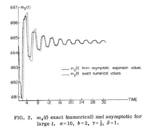
Figure 14.4: Typical result for the magnetization in the step function magnetic field evolution, taken from the work of Barouch et al. [250]. The qualitative behaviour in the case of finite temperatures ($\beta\equiv 1/k_{B}T=1$) is similar to the quantum case at zero temperature studied here ($\beta=\infty$).

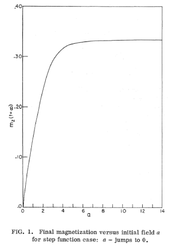
Figure 14.5: Final magnetization in the case of final magnetic field $h_{f}=0$ (step-function magnetic field), taken from the work of Barouch et al. [250]. As seen in Fig.14.6, our $M_{z}(\infty)$ at $T=0$ presents a similar shape.

Although only asymptotic values can be obtained in analytical fashion, we provide here for the sake of completeness a basic strategy to pursue in order to describe the “transient” regime. This is done in order to justify the oscillations seen in Fig.14.3, and following the steps of Barouch et al. [250]. As we can observe, all the time dependence of the purity (14.59) is put in the coefficients $x_{1}^{k}(t)$ (14.65). In order to simplify things, let us consider the fluctuations of the purity $P_{u(N)}(t)$ minus its final value $P_{u(N)}(t\rightarrow\infty)$ in the form $\Delta P_{u(N)}(t)$ (there is an additional static term $\Delta P_{0}$ which is not considered). Simplifying a bit more, let us consider the case $\gamma=1$. We thus have

$$\Delta P_{u(N)}(t)=\frac{4}{N}\sum_{k}[A(k)+B(k)\cos(\omega_{k}t)]\cos(\omega_{k}t),$$ (14.72)

where $A(k)$ and $B(k)$ are some functions of $k$ and the frequency (14.64)

$$\omega_{k}=\sqrt{4(4g\sin k)^{2}+(4\big{(}2g\cos k-h_{f})\big{)}^{2}}$$ (14.73)

is expressed in terms of the final magnetic field $h_{f}$, the interaction strength $g$ and the momenta $k$. Equation (14.72) suggests that we can consider $\Delta P_{u(N)}(t)$ in the thermodynamic limit $N\rightarrow\infty$ (sums become integrals) as the real contribution of a more general equation, namely

$$\Delta P^{{\rm th.}}_{u(N)}(t)\,=\,4\,{\rm Re}\bigg{(}\frac{1}{2\pi}\int_{0}^{\pi}dk[A(k)+B(k)\cos(\omega_{k}t)]\,\,e^{i\,t\,\omega_{k}}\bigg{)}.$$ (14.74)

Following the steps in [250], further changes of variables may lead to an integration in the complex plane following a given path, depending on the values of the poles, which in turn depend on the relative values of final and initial magnetic fields and the strength $g$. Although the solution to (14.74) is rather complex, it is plausible that the solution for either $P_{u(N)}(t)$ or $M_{z}(t)$ drawn in Fig.14.3 represents a special combination of time-dependent functions, but with one definite frequency. As a matter of fact, one can check from inspection that the overall period of oscillation is pretty much the same for all times. In the discussion by Barouch et al. [250], several frequencies are involved. At zero temperature, we pretty much obtain the same results. See Figs. 14.4 and 14.5.

It is likely that the best way to discuss the equilibrium state is to evaluate the time average of expressions (14.59) and (14.60). These curves are shown in Fig.14.6. We plot the asymptotic equilibrium ($t=\infty$) values for the purity (14.59) and magnetization (14.60) with $\gamma=\frac{1}{2}$, $g=-\frac{1}{4}$, versus the initial magnetic field $h_{0}$ and zero final magnetic field $h_{f}$ (step function magnetic field). We notice from inspection that the equilibrium purity also detects a change of regime at $h_{0}=2g=-0.5$, where the function has no well defined derivative. As we approach zero magnetic field, we recover the expected value $P_{u(N)}(t=\infty)\,|_{h_{f}=0}=1/(1+\gamma)$. Also, regarding the magnetization, this is the asymptotic value reached when $h_{0}\rightarrow-\infty$. The magnetization approaches a zero value as $h_{0}$ goes to zero, as it should be. The $\gamma=1$ case is analytic (other cases most probably not). The purity versus $h_{0}$ for a zero final magnetic field $h_{f}$ reads

$$P_{u(N)}(h_{0};t=\infty)\,|_{\gamma=1} = -{\frac{3}{512}}\,{\frac{{h_{0}}^{4}}{{g}^{4}}}+{\frac{1}{128}}\,{\frac{{h_{0}}^{2}}{{g}^{2}}}+{\frac{17}{32}}+{\frac{3}{512}}\,{h_{0}}^{5}{g}^{-5}$$ (14.79)

$${\frac{1}{\sqrt{{\frac{{h_{0}}^{2}}{{g}^{2}}}-8+16\,{\frac{{g}^{2}}{{h_{0}}^{2}}}}}}-1/32\,{h_{0}}^{3}{g}^{-3}{\frac{1}{\sqrt{{\frac{{h_{0}}^{2}}{{g}^{2}}}-8+16\,{\frac{{g}^{2}}{{h_{0}}^{2}}}}}}+$$

$$1/16\,h_{0}{g}^{-1}{\frac{1}{\sqrt{{\frac{{h_{0}}^{2}}{{g}^{2}}}-8+16\,{\frac{{g}^{2}}{{h_{0}}^{2}}}}}}-$$

$$1/2\,g{h_{0}}^{-1}{\frac{1}{\sqrt{{\frac{{h_{0}}^{2}}{{g}^{2}}}-8+16\,{\frac{{g}^{2}}{{h_{0}}^{2}}}}}}-3/8\,{\frac{{g}^{2}}{{h_{0}}^{2}}}+$$

$$3/2\,{g}^{3}{h_{0}}^{-3}{\frac{1}{\sqrt{{\frac{{h_{0}}^{2}}{{g}^{2}}}-8+16\,{\frac{{g}^{2}}{{h_{0}}^{2}}}}}}.$$

Its derivative has a finite value at the critical point $\frac{h_{0}}{2g}$, though it is discontinuous

$$\frac{dP_{u(N)}(h_{0};t=\infty)}{dh_{0}}|_{h_{0}/2g\rightarrow 1^{\pm}}=-\frac{1}{16}\frac{\mp 4+(\frac{1}{g^{2}})^{\frac{3}{2}}g^{3}}{(\frac{1}{g^{2}})^{\frac{3}{2}}g^{4}}.$$ (14.80)

These features transpire from Fig.14.6, computed for the $\gamma=\frac{1}{2}$ case. In fact, the magnetization $M_{z}(t=\infty)\,|_{h_{f}=0}$ possesses an analytic expression as well, but it is not given due to its complex form.

Figure 14.6: Asymptotic (or stationary) values for $P_{u(N)}(t=\infty)$ and $M_{z}(t=\infty)$ for the step-function magnetic field $h(t)$ instance, plotted as a function of the initial $h_{0}$, with $h_{f}=0$, $\gamma=\frac{1}{2}$ and $g=-\frac{1}{4}$. $M_{z}(t=\infty)$ smoothly tends to zero, while $P_{u(N)}(t=\infty)$ still detects the critical point $h_{0}=2g=-0.5$ (vertical line). See text for details.

It is clear from the previous formulas that, although we reach an equilibrium value for $M_{z}(t=\infty)\,|_{h_{f}=0}$, this is different from zero and depends on the initial magnetic field $h_{0}$ as prescribed by relation (14.2.2). This is the conclusion reached by Barouch et al. in [250] at finite temperatures, extended here to the case of zero temperature. What is also surprising is the fact that the own measure of entanglement $P_{u(N)}$ reaches an equilibrium value, which implies that not only the magnetization presents a non-ergodic behaviour, but entanglement itself too.


Exponential decay

In this case, $g(t)=g_{0}$ and

$$h(t)=\left\{\matrix{h_{0}&t\leq 0\cr h_{f}+(h_{0}-h_{f})e^{-\kappa t}&t>0}\right.,$$ (14.81)

where $\kappa$ plays the role of a knob adjusting the speed of the passage. Then, Eqs. 14.56 are ($t>0$)

$$\left\{\matrix{\dot{x}_{1}(t)=2\tilde{\alpha}x_{2}^{R}(t)\cr\dot{x}_{2}^{R}(t)=\tilde{\alpha}-2\tilde{\alpha}x_{1}(t)-\beta(t)x_{2}^{I}(t)\cr\dot{x}_{2}^{I}(t)=\beta(t)x_{2}^{R}(t)}\right.$$ (14.82)

where $\tilde{\alpha}=4g_{0}\gamma\sin k$, $\beta(t)=\beta_{a}+\beta_{b}z$, with $\beta_{a}=-4(2g_{0}\cos k-h_{0})$, $\beta_{b}=4(h_{f}-h_{0})$, and $z=1-e^{-\kappa t}$. (Again, the indices $R,I$ denoting the real and imaginary parts of $x_{2}$, respectively.) In terms of the variable $z$, Eqs. 14.82 read ($\partial_{t}=\kappa(1-z)\partial_{z}$)

$$\left\{\matrix{\kappa(1-z)\dot{x}_{1}(z)=2\tilde{\alpha}x_{2}^{R}(z)\cr\kappa(1-z)\dot{x}_{2}^{R}(z)=\tilde{\alpha}-2\tilde{\alpha}x_{1}(z)-\beta(z)x_{2}^{I}(z)\cr\kappa(1-z)\dot{x}_{2}^{I}(z)=\beta(z)x_{2}^{R}(z)}\right.$$ (14.83)

where the derivatives are now with respect to the variable $z$. The solution to Eqs. 14.83 can be obtained proposing an ansatz function of the form $x_{2}^{R}=\sum_{m}a_{m}z^{m}$, where the coefficients $a_{m}$ are related by a recurrence relation, obtained when inserting the ansatz in Eqs. 14.83 and keeping the same order terms in both hands of the Eqs. However, this recurrence relation is not simple and a straight computation of the $h$-purity and magnetization using numerical methods was performed.

In Fig.14.7 we show the time-dependent $u(N)$-purity and magnetization (Eqs. 14.59 and 14.60, respectively) for $g_{0}=-1/4$, anisotropy $\gamma=1$, and for $\kappa=1$, $\kappa=10$, and $\kappa=150$. For a slow passage ($\kappa=1$), an equilibrium value is steadily and monotonically reached. No oscillations appear in this case. On the contrary, as we increase $\kappa$, $P_{u(N)}(t)$ and $M_{z}(t)$ present oscillations around their limiting values $P_{u(N)}(t=\infty)$, $M_{z}(t=\infty)$. A very fast passage ($\kappa=150$) virtually coincides with a step function behaviour in $h(t)$, and the result is equivalent to the one showed in Fig.14.3.

Figure 14.7: Time-dependent $u(N)$-purity (solid lines) and magnetization (dashed lines) of the evolved state for the exponential-decay case for different values of the exponent $\kappa$. The initial and final magnetic fields are $h_{0}=-5$ and $h_{f}=-1$, respectively.

As far as non-ergodicity is concerned, we appreciate also in Fig.14.7 that both $P_{u(N)}(t)$ and $M_{z}(t)$ tend to a stationary equilibrium which is non-ergodic, independently of the parameter $\kappa$. It is plausible to assume then that this is a special feature independent on the specific time evolution employed.


Hyperbolic magnetic field

In this case, $g(t)=g_{0}$ and the time-dependent magnetic field is

$$h(t)=\left\{\matrix{h_{0},&t\leq 0\cr h_{f}+\frac{(h_{0}-h_{f})}{1+t},&t>0}\right..$$ (14.84)

The solutions to Eqs. 14.56 are obtained similarly to the exponential-decay case by proposing an ansatz of the form $x_{2}^{R}(t)=\sum_{m}a_{m}t^{m}$ and obtaining a recurrence relation for the coefficients $a_{m}$. As in the exponential-decay case, we did not obtain the exact solution since numerical methods allow us to compute the time-dependent $h$-purity and magnetization directly, efficiently, and with high accuracy.

In Fig.14.8 we show the time-dependent $u(N)$-purity and magnetization for $g_{0}=-1/4$, $h_{0}=-5$, and $h_{f}=-1$ (the same values used in the step function case), and with anisotropies $\gamma=0.5,1$. It is remarkable from inspection that both the purity and magnetization do not present oscillations, and the tendency to reach a stable value is slowed down. Again, and with a different time dependence in $h$, the non-ergodic features of $P_{u(N)}$ and $M_{z}$ are apparent as $t\rightarrow\infty$. We see that low $\gamma$-values is tantamount as high values of $P_{h}$ and $M_{z}$.

Figure 14.8: Time-dependent $u(N)$-purity (solid lines) and magnetization (dashed lines) of the evolved state for the hyperbolic-function case. Similarly to the step-function case, the interaction coefficients are $g_{0}=-1/4,h_{0}=-5,h_{f}=-1$.

14.2.3 Adiabatic evolution: recovering the static case

As mentioned above, in [245] the $u(N)$-purity was computed for the static anisotropic $XY$ model in a transverse magnetic field as a function of the coupling constant $g$ and for $h=1$. Remarkably, the $u(N)$-purity characterizes the QPT present in this model, changing drastically at the critical point $g_{c}=1/2$. Now, a question arises: Do we observe a QPT when a time dependence is involved? In other words, does the speed of passage through the critical point influence the very existence of a QPT? One would expect then to answer these questions by studying the behaviour of the relative purity $P_{u(N)}(t)$.

An interesting issue appears when one considers slow evolutions. The adiabatic theorem states that if the time-dependent Hamiltonian $H(t)$ of a system evolves slow enough and no level crossing with excited states exists, the ground state remains as such with time. In fact, this is the case in the time-dependent anisotropic $XY$ model in a transverse magnetic field. Therefore, one should expect to recover the static case for slow evolutions of the time-dependent parameters in $H(t)$.

For the sake of simplicity and without loss of generality, let us focus our attention in the Ising model in a transverse constant magnetic field; i.e., $\gamma=1$ and $h(t)=1$ in Eq. 14.37. The time-dependence now is in the coupling parameter $g(t)$. Although experimentally is more feasible to vary the external magnetic field, the conclusions in both cases are the same. Let us consider then the following time evolution for $g(t)$:

$$g(t)=\left\{\matrix{g_{0},&t\leq 0\cr g_{f}+(g_{0}-g_{f})\exp(-\kappa t),&t>0}\right.,$$ (14.85)

with $g_{0}=0$ and $g_{f}=1$. In this way, the critical point $g_{c}=1/2$ is crossed at a speed given by $\kappa$. Again, the time dependent $u(N)$-purity can be numerically computed by inserting $g(t)$ in Eqs. 14.56 and then inserting the corresponding solutions $x_{1}^{k}(t)$ in Eq. 14.59.

In Fig.14.9 we show $P_{u(N)}(t)$ as a function of $g$ and for $\kappa=10^{-3}$, 0.01, 0.1, 1, and $10$. The static case corresponds to the dashed thin line (see [245]). We observe that the curves corresponding to the slow-speed cases with $\kappa=10^{-3}$ (solid thick line) and $\kappa=0.01$ (dot dashed thick line) are very close to the static case, as stated by the adiabatic theorem. In the inset a) the region around the critical point is enhanced. The average final value for the $\kappa=10^{-3}$ case is 0.496, remaining extremely close to $g_{c}=1/2$. On the other hand, fast-speed evolutions are shown in the inset b), where no obvious critical point is detected through the $u(N)$-purity.

Figure 14.9: Time-dependent $u(N)$-purity of the evolved state for an exponential-like passage through the critical point $g_{c}=1/2$. For slow passages $\kappa\rightarrow 0$ the static case (dashed lines) is recovered and the $u(N)$-purity behaves as a disorder parameter. Inset a shows the details around the critical point $g_{c}=\frac{1}{2}$. As we slow down the passage through the critical point, we get closer and closer to the static case, given by Eq. (14.34). For fast passages (inset b) we no longer agree with the static case. Here $h(t)=1$ and $\gamma=1$. $\kappa=10^{-3}$ (solid thick line) is very close to the static case, which is in full agreement with the adiabatic theorem.

14.3 Concluding remarks

This Chapter has been devoted to the application of the notion of Generalized Entanglement (GE) to broken-symmetry QPTs. As we focused on a situation where the physically relevant observables form a Lie algebra, a natural GE measure provided by the relative purity of a state relative to the algebra has been used in order to identify and to characterize these transitions. Therefore the measure employed in order to detect a QPT was the purity $P_{h}$ relative to a set of observables $h$, which form a Lie algebra. We recall that the concept of $h$-purity encompasses the usual notion of entanglement if the family of all local observables is distinguished. In addition, the possibility to directly apply the GE notion to arbitrary quantum systems, including indistinguishable particles, becomes apparent when using a fermionic system as a relevant case study, as it is the case here.

The study performed in [245] dealt with different exact lattice models in the application of $P_{h}$ in a context of QPT. In this Chapter we have first focused on a new lattice model which, to our knowledge, had not been solved analytically to date: the anisotropic $XY$ model with bond alternation in a transverse magnetic field. The analytical detailed resolution of this system is done for pedagogical reasons, because in the end we provide a formula for the evaluation of the purity $P_{h}$ relative to the $h=u(N)$ algebra of observables. The calculation of $P_{h}$ is performed numerically, but one must not rule out the possibility that it might admit an analytical expression in the thermodynamic limit $N\rightarrow\infty$, where $N$ is the number of lattices. However the concomitant phase diagram of this bond-alternating model is obtained in analytical fashion, and one can easily recover the usual anisotropic $XY$ model with a transverse magnetic field studied in [245]. The derivative of $P_{h}$ with respect to some parameter in the phase diagram “signals” the presence of a QPT, in complete agreement with analytic results.

In a second stage, we abandon the static description of QPT and GE through the study of the purity $P_{h}$ relative to the $h=u(N)$ and we let the time run. The goal was to study the dynamic entanglement features of the usual anisotropic $XY$ model when we let the coupling constant $g$ and the external, transverse magnetic field depend on time ($g(t),\,h(t)$). First, we found the general time dependent differential equations for the coefficients describing the ground state $|\Psi(t)\rangle$ of the system, for arbitrary $g(t),\,h(t)$. Then we calculated the purity $P_{u(N)}(t)$ and the magnetization $M_{z}(t)$ setting $g(t)=g_{0}$ and considering different cases for the time dependent magnetic field $h(t)$, namely, i) step function, ii) exponential and iii) hyperbolic. In the step function case, the equations for the ground state of the system can be found analytically, but the time dependent $P_{u(N)}(t)$ and $M_{z}(t)$ ought to be calculated numerically. However, for certain values of the parameters of the system Hamiltonian, the equilibrium values $P_{u(N)}(t\rightarrow\infty)$ and $M_{z}(t\rightarrow\infty)$ can be expressed in analytical fashion only in the step-function magnetic field $h(t)$ instance. Yet, at zero temperature, the magnetization reaches a final non-zero value for all $h(t)$ cases considered, which means that $M_{z}(t)$ is non-ergodic: it strongly depends on the initial values. This fact was already known to Barouch et al. in [250, 251] back in the 70s for the same system at finite temperatures. Here we show that it is indeed the same case for $T=0$.

But the magnetization is not the only non-ergodic quantity here. Entanglement itself ($P_{u(N)}(t)$) pretty much behaves as the magnetization $M_{z}(t)$, that is, it is also non-ergodic. This fact is certainly relevant, for entanglement –understood in the framework of the theory of GE– do behaves as a property of the system, similarly to the magnetization on equal footing.

Finally, we wanted to study the counterpart of previous sudden changes in the parameters $g(t),\,h(t)$. An interesting issue appeared when we considered slow evolutions. The adiabatic theorem states that if the time-dependent Hamiltonian $H(t)$ of a system evolves slow enough and no level crossing with exited states exists, the ground state remains as such with time, and in fact this was the case in the time-dependent anisotropic $XY$ model in a transverse magnetic field. Therefore, one expected to recover the static case for slow evolutions of the time-dependent parameters in the Hamiltonian $H(t)$. By varying the coupling constant $g(t)$ exponentially, with $h(t)=1$ we compared the different results for the purity $P_{u(N)}(t)$ vs. $g(t)$. For different speed passages trough the critical point $g_{c}=\frac{1}{2}$, we show in the “frozen” plot $P_{u(N)}(t)$ vs. $g(t)$ how it approached the static result for extremely slow passages, agreeing with the adiabatic theorem.

Although not discussed in this thesis it is worth commenting on the following important issue. As pointed out in [245], in general terms to determine in a systematic way the minimal subset of observables $h$ whose purity is able to signal and characterize the QPT, and thereby providing the relevant correlations, requires an elaborate analysis. Going one step further, it is perhaps even more interesting to study the open question of finding the minimal number of GE measures, possibly including measures of GE relative to different observable sets, needed to unambiguously characterize a QPT, in terms of critical exponents, university classes, etc. However, this may constitute a subject of future study. A motivation to study the model Hamiltonian of Eq. (14.6) was precisely the investigation of a problem with various order parameters that would help us figuring out the systematic choice of minimal algebras.

Note added. After completion of this work, it was brought to our attention the fact that non-ergodicity was discovered also in [262] for finite temperatures in the bipartite entanglement (the concurrence to be more precise) present between two sites in the $XY$ model.

Part IV Conclusions

Throughout the present Thesis we have emphasized the role played by information or entropic measures in the characterization of quantum entangled states. The correct use of MaxEnt procedures, subject to certain requirements, turned out to be a powerful and safe inference tool (safe in the sense of not “faking” the entanglement present in a given state $\rho$). Thus Jaynes’ principle is universally valid as long as we identify the correct input information. Also, the classic $q$-entropic inequalities offer a necessary criterion for separability which has interesting echoes in the volume of states occupied by those which do not violate them, as well as in their connection –chain of implications– with other existing criteria. We have also seen that MEMS states play a distinguished role with regards to the violation of the aforementioned classical entropic inequalities. Besides, we have seen that it is possible to correlate total entropies (its mean value) of states of two qubits with their entanglement. The relationship between entanglement and mixedness has been established, and we have reviewed the pros and cons of different measures in the space of mixed two-qubit states. In this vein, the structure of two-qubit mixed states in connection with mixedness and entanglement appears slightly different when a different generation of states is performed. In clear connection with quantum computation, the entanglement distribution of quantum gates and their entangling power acting on pure or mixed two-qubit states has been investigated as well.

Regarding the characterization of entanglement, we have seen that it constitutes an essential ingredient in certain quantum algorithms such as Grover’s and, among other properties, we explicitly have shown that entanglement-assisted time evolution of states towards orthogonal ones does not occur in the case of indistinguishable particles, at least for fermions. Entanglement, in the particular form the so called purity, can also describe condensed matter systems. Particularly, we have seen that there exists a connection between quantum phase transitions (QPTs) and entanglement in the $XY$ bond alternating anisotropic model with a transverse magnetic field. By studying the dynamical evolution of the $XY$ anisotropic model, we have discovered interesting non-ergodic properties of the purity measure, which reinforces our perception of entanglement as a property that characterizes the quantum system, specially in broken-symmetry QPTs, signalling the position of the existing critical points.

Summing up, the most important results of this Thesis appear as follows:

• Jaynes’ principle does not “fake” entanglement. We have exhaustively investigated Horodecki’s “fake” inferred entanglement problem, related with the use of the maximum entropy principle, with reference to distinct inference schemes, and advanced a new one, reminiscent of Horodecki’s, for dealing with general observables.

• Inclusion relations between several separability have been checked numerically. We have explored the application of different separability criteria by recourse to an exhaustive Monte Carlo exploration involving the pertinent state-space of pure and mixed states. The corresponding chain of implications of different criteria has been in such a way numerically elucidated. Besides, we have quantified for a bipartite system of arbitrary dimension, the proportion of states $\rho$ that can be distilled according to a definite criterion.

• We have extensively explored all possible connections of the so called $q$-entropic information measures and their connection with entanglement. Secondly, the connection with entanglement and mixedness has been studied too. Also, we focused our attention on the interesting properties that link a particular class of states, the so called Maximally Entangled Mixed States (MEMS), with the violation of the usual entropic inequalities.

• The relationship between entanglement and purity of states of two-qubit systems has been revisited in the light of the $q$-entropies as measures of the degree of mixture. Probability distributions of finding quantum states of two-qubits with a given degree of mixture have been analytically found for $q=2$ and $q\to\infty$. We claim that $\lambda_{m}$ itself constitutes a legitimate measure of mixture.

• The space $\mathcal{S}$ of mixed states ot two-qubits is not very sensitive, with regards to the concomitant entanglement-mixedness properties of states, to the measure used to generate them.

• We have focused our attention on the action of quantum gates as applied to multipartite quantum systems and presented the results of a systematic numerical survey. We also studied numerically some features of the probabilities of obtaining different values of $\Delta E$. Quantum gates are more efficient, as entanglers, when acting upon states with small initial entanglement, specially in the case of pure states.

• There is a clear correlation between the amount of entanglement and the speed of quantum evolution for systems of two-qubits and systems of two identical bosons. On the contrary, such a clear correlation is lacking in the case of systems of identical fermions.

• There exists a clear connection between quantum phase transitions and entanglement, as expressed by the so called purity measure, a generalized entanglement measure. We have obtained –to our knowledge for the first time– the phase diagram of a bond alternating $XY$ model and checked that the purity, or its derivative to be more precise, detects too the critical points in a richer phase diagram. Finally, the dynamic evolution of the $XY$ anisotropic model in a transverse magnetic field reveals that entanglement itself, applied in a condensed matter scenario, can present non-ergodic features.

OPEN QUESTIONS AND FUTURE WORK

The field of quantum information theory and quantum computation is growing extremely fast, so quickly that it is difficult to compile all the relevant results that constantly appear in the vast literature of this newborn branch of theoretical and experimental physics. It is likely that no other field of physics had experienced before such a rapid theoretical and experimental development as it is happening with quantum information theory. Quantum communication, quantum teleportation and quantum computation are the main focus of experimental efforts. The promise of a secure communication and ultrafast computations is a subject that many governments around the world have taken seriously into account. Therefore, lots of related difficulties naturally arise both in the theoretical and experimental implementations of these items, what makes the research in this field more exciting.

However, in the meantime, there have appeared skeptical voices of relevant scientists like Gerard ’t Hooft [263] that conceive the impossibility to overcome the technical difficulties that appear. These criticisms are in the line that no matter how better we improve our technology, there will always appear some quantum limit that cannot be avoided. These limits translate into the fact that quantum information, as we have studied here, will end up being ultimate classical information (the usual bits 0 and 1). Nevertheless, proof-of-principle NMR and ion-trap quantum computing has been observed. So the basis for quantum computation exists. However, serious drawbacks are present when the experimentalist wants to isolate the system of qubits he/she is interested in from the rest of the universe. Decoherence times ought to be great enough so that a quantum gate operation can be performed. Tailoring interactions between subsystems, which is tantamount as engineering entanglement, constitutes a difficult issue. That is why new proposals for quantum computing appear from time to time. Physicists seek out potential proposals (physical systems) for quantum bits, such as the combined system of the spin of a nucleous and the one of the electrons surrounding it, that fulfils the requirements of DiVincenzo’s criteria (see Chapter 2). Such systems do exist, but we are still unable to handle them in the way which is required. Difficulties are of technical nature. Another kind of criticism is the one against the object of studying algorithms and protocols in quantum computation and quantum communication, respectively. One could argue what is the purpose of studying processes that should still wait to be observed and controlled. This remark is, in fact, a confirmation that theoretical progress grows at a different rate as compared to the experimental stuff. It confirms, in turn, the huge interest that is growing in the physics community about these extraordinary quantum features.

But again, would not it be easier to still consider classical information and build classical computers with one electron transistors, instead of complex, strange proposals that may not in the end work? Perhaps this is a short-term solution. It would make no use of entanglement whatsoever. Entanglement, what for? Well, it makes no reference to the inherent randomness of quantum mechanics. This fact means that it does not support any device that provides one with absolutely secure communication, as quantum cryptography is experimentally giving nowadays. Quantum teleportation? No pink!

Quantum computers are the definitive, once-for-all, long standing solutions to simulate quantum physics. Would not it be marvellous that one could map a quantum physical system like a cuprate superconductor into another quantum physical one like a quantum computer? If this were possible, one could simulate the intriguing features of non-understood phenomena so that we would get a better insight: to calculate the theoretical mass of the proton, to make precise meteorological predictions nearly in real time, and the list continues..

Finally, here come the one-million-dollar questions: what if a quantum computer can not be built? What if we cannot control undesired interactions or instabilities? What if none of the proposals for quantum computing scales the number of qubits up to no more than a certain small number? What if we end up with a system that, yes, can perform better that a supercomputer, but not as much as we expected? Have we wasted precious time for nothing? Well, it is a common belief, and I shared that impression, that to build a quantum computer is not the ultimate goal. Never in the past a pure theoretical concept such as non-locality –crystallized into entanglement– gathered different disciplines altogether (computer science, information theory, quantum mechanics and its foundations..) around this strange quantum correlation. As pointed out by Schrödinger [2], quantum entanglement is not a feature of quantum mechanics, but rather the characteristic feature that makes quantum mechanics different from classical physics. As a consequence, it deserves to be studied in all possible ways. It constitutes, in the modern context of science, a clear example that fundamental or pure research need not has to find an application. But if it eventually does, the results become superb.

Now then, let us return from the future.. In this final Chapter we will not be dealing with the challenges that appear in the previous fields, mainly because we have not studied them in any way. Instead, we expose those problems that appear in basic research that we have dealt with in this Thesis. It’s about a better understanding of the physical nature of entanglement, its detection and characterization in different contexts.

Detection of entanglement

In the context of the orthodox view of unentangled states of $N$ parties,

$$\rho\,=\,\sum_{k}p_{k}\,\rho^{(k)}_{1}\otimes...\otimes\rho^{(k)}_{N}$$ (14.86)

with $0\leq p_{k}\leq 1$ and $\sum_{k}p_{k}=1$, there is no definitive criterion yet which can asserts if a given state $\rho$ can be written in the form (14.86) or not, even in the general case of bipartite systems of arbitrary dimensions. The application in this case of the theory of positive maps advanced by the Horodecki family [140], turns out to be a hard problem to solve, and possibly may not have a solution. Also entanglement witnesses, which have proved to be quite successful, find it hard to go up to high dimensions. Indeed, much effort is done by many authors in order to find a solution to the separability problem as we present it here, but a conclusive answer still remains, at least for mixed states. In practice, what has been done in order to tackle the problem is to induce partitions in the system, that is, to consider bipartite entanglement –which is well understood– between clusters of particles. Certainly this may not be a definite solution, because the problem of characterizing genuine multipartite entanglement still resists, in spite of many efforts [264, 265, 266].

Motivated by these facts, one may wonder if the entropic criteria could shed some light on the problem. These simple, information-theoretical based criteria is endowed with the high physical and intuitive notion that the entropy of the total system, as described by the density matrix $\rho_{1,..,N}$, has to be greater that any of its subsystems for classical systems, but entangled states are so particular that this may happen or not. Therefore, we consider a subject of future study the derivation of general conditions for positivity using the entropic inequalities. This procedure should involve the characterization of the positivity of $2^{N}-2$ inequalities, with $N$ being the number of parties.

Characterization of entanglement

As we have seen, the parameterization of the two-qubit space ${\cal S}$ of all pure and mixed states (see also the Appendix) has been made upon the assumption that states are distributed according to a definite measure. In the case of pure states, the only possible measure happens to be the Haar measure for unitary matrices. In this case, many average quantities such as the mean degree of mixture $R=1/Tr\,(\rho^{2})$, or even the distribution of concurrence squared $C^{2}$ ($P(C^{2})$) can be found in analytical fashion. But when it comes to mixed states, the situation is more involved. The computation of the aforementioned (average) quantities characteristic of the space ${\cal S}$ is three-fold complex: firstly, i) there is no unique procedure to generate those mixed states, because one can choose different distributions for the simplex $\Delta$ describing the eigenvalues of the state $\rho$; secondly, ii) the final chosen distribution for $\Delta$ may or may not induce a real metric in the 15-dimensional space of two-qubits ${\cal S}$; and finally, iii) in either cases the computation of several properties has to be performed in numerical fashion.

If we were able to describe analytically several properties in this 15-dimensional space of two-qubits ${\cal S}$, which is the simplest one exhibiting the feature of entanglement we could gain, on the one hand, more physical insight into features such as the geometrical meaning of positive partial transposition of $\rho$, and on the other hand, simplicity in the numerical generation of states. In the latter case, a clear example of this situation is encountered whenever we want to calculate distance measures as in the case of the minimum distance to a completely separable matrix as a measure of separability. This is indeed the case for the so called robustness of entanglement or the relative entropy of entanglement introduced in Chapter 5, which do not possess an analytical formula to date.

In order to overcome this facts for two-qubit systems, an interesting parameterization of bipartite systems based on SU(4) Euler angles has been introduced recently by T. Tilma et al. in [267]. Such a parameterization should be very useful for many calculations, especially numerical, concerning entanglement. This parameterization would also allow for an in-depth analysis of the convex sets, subsets, and overall set boundaries of separable and entangled two-qubit systems. This simplification in the calculations, which could be done analytically, is certainly of interest for us and will be explored in the future.

The measure $d$ described in Chapter 12 in order to analyse genuine multipartite pure state entanglement

$$0\,\leq\,d\equiv C^{2}_{1(2..N)}-\sum_{i=2}^{N}C^{2}_{1i}\,\leq\,1,$$ (14.87)

$N$ being the number of qubits in a pure state $\rho=|\Psi\rangle_{1..N}\langle\Psi|$, and $C^{2}_{xy}$ stands for the concurrence squared between qubits $x,y$, opens a new window to the study of the evolution of entanglement during the application of a given quantum algorithm.

Along this line, it is of interest also to study the time evolution of pure states of $N$ parties, in similar fashion as done in Chapter 12 for two-qubit systems. Several efforts have been already done in systems of two-qutrits and three qubits. Although some results can be obtained analytically, it is clear than a direct relation between measure (14.87) and the time evolution towards an orthogonal state will not be of trivial nature at all. Besides, one has to bear in mind that the results reported in the literature [45, 240] deal with special forms of states, which allow an analytical study. The relation between global properties of the set of pure and mixed states of $N$ parties, on the one hand, and the role of entanglement in the concomitant time evolution, one the other hand, will certainly deserve further exploration.

It is implicit from (5.1) that the $N$ parties of this composite system, whose state $\rho$ belongs to the Hilbert space ${\cal H}={\cal H}_{1}\otimes...\otimes{\cal H}_{N}$, are distinguishable or, on the contrary, are indeed identical but can be addressed individually because the individual wavefunctions do not overlap. This is certainly the case for quantum communication, teleportation, and quantum cryptography, because communication only occurs between two parties that are far apart from each other. Therefore we do not have to worry about the statistics of the particles involved (either bosons or fermions). In Chapter 14 we saw that entanglement plays a decisive role in a faster evolution of a pure state to an orthogonal one. In view of this fact, one is naturally led to encounter an experiment which, by indirect means, could detect the presence of entanglement if the time evolution of a given state to its orthogonal one is speeded-up. In the same spirit, we encountered in Chapter 14 that this pattern did not work for fermions. We did not find a direct correlation whatsoever between entanglement and time evolution. We will look in the future for the solution to this puzzle.

Appendices

14.4 A. Landmarks in classical and quantum information theory

Here is a brief account of the most significant discoveries occurred in the fields of Information Theory, Computer Science and Quantum Information Theory. The list of the modern achievements in quantum information (a field growing rapidly and in constant change) presented here is far for complete. Thus, the following references could serve as guideline where the correlations between several disciplines become apparent with time. Those facts specially related to entanglement-separability appear underlined.

• 1870 J. C. Maxwell: public appearance of Maxwell’s demon in the Theory of Heat. Probably the resolution of a paradox in physics had never been so fruitful before as Maxwell’s demon

  
  

  “Now let us suppose that such a vessel is divided into two portions, A and B, by a division in which there is a small hole, and that a being… opens and closes this hole, so as to allow only swifter molecules to pass from A to B… He will thus, without expenditure of work, raise the temperature of B and lower that of A, in contradiction to the second law of thermodynamics”

• 1929 L. Szilard: Über die Entropieverminderung in einem thermodynamischen System bei Eingriffen intelligenter Wesen. Seminal paper relating the Maxwell paradox to entropy and information. Besides, the point stressed by Szilard was that information (not yet defined as such) is linked to a physical representation, pioneering future disciplines describing the intimate connection between physics (classical and quantum), information and computation

  
  

  “If we do not wish to admit that the Second Law has been violated, we must conclude that the intervention which establishes the coupling (the measuring instrument and the thermodynamic system) must be accompained by a production of entropy”

• 1932 J. von Neumann: Mathematische Grundlagen der Quantenmechanik. Seminal work in quantum mechanics, revisits his introduction of the thermodynamical entropy $S(\rho)$ through the formalism of density matrices. Introduction of the measurement theory

• 1935 A. Einstein, B. Podolsky and N. Rosen: Can Quantum-Mechanical Description of Physical Reality Be Considered Complete? Keystone paper in the foundations of quantum mechanics. Based in position-momentum arguments of two distant particles, it raised the question of whether Nature can be regarded as locally realistic as opposed to non-local or “incomplete”. The modern version with spins is due to D. Bohm (1951)

• 1935 E. Schrödinger: Die gegenwärtige Situation in der Quantenmechanik. Seminal paper where Verschränkung (German word for “folding arms”) or entanglement is introduced as “the characteristic trait of quantum mechanics”

  
  

  “When two systems, of which we know the states by their respective representatives, enter into temporary physical interaction due to known forces between them, and when after a time of mutual influence the systems separate again, then they can no longer be described in the same way as before… By the interaction, the two representatives (or $\Psi$-functions) have become entangled”

• 1936 A. M. Turing, On Computable Numbers, with an Application to the Entsheidungsproblem. Keystone paper in computation science. He poses the basic operating principles (further developed by von Neumann) of the ordinary computers (birth of the Turing machine). Together with A. Church they formulate what is known as the “Church-Turing hypothesis”: every physically reasonable model of computation can be efficiently simulated on a universal Turing machine

• 1949 C. E. Shannon and W. Weaver: The Mathematical Theory of Communication. Seminal paper in information theory

• 1957 E. T. Jaynes: Information Theory and Statistical Mechanics. The principle of maximum (informational) entropy is advanced as the basis of statistical mechanics

  
  

  “Information theory provides a constructive criterion… which is called the maximum-entropy estimate… If one considers statistical mechanics as a form of statistical inference rather than a physical theory… the usual rules are justified independently of any physical argument, and in particular independently of experimental verification”

• 1959 R. P. Feynman: There is Plenty of Room at the Bottom. Briefly exposes the fact that there is nothing in the physical laws that prevents from building computer elements enormously smaller than they are (or were). Constitutes the first wink to the physical limits of computation

• 1961 R. Landauer: Irreversibility and Heat Generation in the Computing Process. R. Landauer formulated his celebrated principle, stating that in order to erase one bit of information it is necessary to dissipate an amount of energy equal to $\ln 2\,k_{B}T$, where $k_{B}$ is Boltzmann’s constant, and $T$ is the temperature at which the computing device is working.

• 1964 J. S. Bell: On the Einstein-Podolsky-Rosen paradox. Milestone paper in quantum mechanics. J. Bell proposes several inequalities in order to test whether Nature admits local realism or follows the tenets of quantum mechanics. The most famous inequality, the Clauser-Horne- Shimony-Holt (CHSH) inequality follows from Bell’s work. In the forthcoming decades experimental setups will support Bell’s view

• 1973, 1982 C. H. Bennett. Inspired by R. Landauer, Bennett demostrates that reversible, logically and thermodynamically (avoiding erasure), computation (classical) is possible. Reversibility in computation is first considered. It naturally arises when quantum gates are considered (unitary operations). Later on Maxwell’s demon is exorcised using his memory erasure (the demon must store the information obtained)

• 1982 R. P. Feynman: Simulating Physics with Computers. Quantum mechanical phenomena are extremely difficult (if not impossible) to simulate on a digital (or classical) computer

• 1982 W. K. Wootters and W. H. Zurek: A single quantum cannot be cloned. Simple but extremely important demonstration of the Non-Cloning Theorem. Its consequences range the whole quantum information field

• 1984 C. H. Bennett and G. Brassard: Quantum cryptography: Public key distribution and coin tossing. Seminal paper, one of the first comprehensive protocols for quantum cryptography. Work followed by a series of fascinating experiments demonstrating quantum cryptography (entanglement is essential) at very long distances (Gisin group in Geneva)

• 1985 D. Deutsch: Quantum theory, the Church-Turing principle and the universal quantum computer. Milestone paper, it constitutes the first formal bridge between quantum mechanics and computation science. Machines rely on characteristically quantum phenomena to perform computations, or in other words, the abstract mathematical idea of logical action during computation depends on the physical support. Recall, in a similar analogy, that geometry turned out to be falsable only in a physical context (General Relativity Theory)

• 1989 R. F. Werner: Quantum states with Einstein-Podolsky-Rosen correlations admitting a hidden-variable model. Entangled states are strange: they can be entangled and satisfy general Bell inequalities

• 1992 C. H. Bennett and S. J. Wiesner: Communication via one and two-particle operators on Einstein-Podolsky-Rosen states. Paper where the issue of quantum dense coding is discovered and explained

• 1993 C. H. Bennett, G. Brassard, C. Crépeau, R. Jozsa, A. Peres and W. K. Wootters: Teleporting an unknown quantum state via dual classical and EPR channels. Striking paper where quantum teleportation is discovered and explained. Its experimental realization was carried out in 1996 by the group of Anton Zeilenger.

• 1994 P. W. Shor: Algorithms for quantum computation, discrete logarithms and factorizing. The field of quantum computing blossomed into a new era. It was shown that on a (hypothetical) quantum computer there are polynomial time algorithms for factorization and discrete logarithms, impossible to achieve on a universal (classical) Turing machine. This fact implied that all the encryptation codes (based so far on the difficulty of factoring large integers) could be broken easily with the advent of a quantum computer. Factorization is reduced to period-finding

• 1995 D. Deutsch, A. Barenco and A. Ekert: Universality in quantum computation. Fundamental paper where quantum computation is shown to be univeral on almost every two-qubits gate. Generalizes the result by DiVicenzo (1995) that the CNOT plus single qubit gates suffices for universal quantum computation

• 1995 J. I. Cirac and P. Zoller: Quantum Computations with Cold-Trapped Ions. Theoretical proposal for reliable quantum computation based on ions confined in a linear trap. Paper of enormous impact in the experimental realization and study of ion-trapped quantum computers

• 1996 A. Peres: Separability Criterion for Density Matrices. Formulation of the necessary condition for separability for bipartite general states $\rho$ based on the Positive Partial Transposition (PPT) of $\rho$. Peres also gives some examples showing that the PPT criterion is more restrictive than Bell’s inequality, or than the $q$-entropic inequalities provided the same year by the Horodecki family. The same authors showed by the same dates that PPT was a necessary and sufficient separability criterion for $2\times 2$ and $2\times 3$ systems

• 1997 D. Bouwmeester, J. W. Pan, K. Mattel, M. Eibl, H. Weinfurter and A. Zeilinger: Experimental quantum teleportation. The state of polarization of a photon is experimentally teleported. Milestone paper in all fields of physics, that soon will be followed by other groups in the world, using several different techniques (optical, NMR and “squeezed” states of light)

• 1997 L. K. Grover: Quantum mechanics helps in searching for a needle in a haystack. Development of the quantum search algorithm. The improvement versus the classical case is of order $O(\sqrt{N})$. The original work dates back to 1996

• 1998 D. Loss and D. P. DiVincenzo: Quantum computation with quantum dots. Theoretical proposal for quantum computing using spin-based coupled quantum dots

• 2004 M. Riebe, H. Häffner, C. F. Roos, W. Hänsel, J. Benhelm, G. P. T. Lancaster, T. W. Körber, C. Becher, F. Schmidt-Kaler, D. F. V. James and R. Blatt: Deterministic quantum teleportation with atoms. Striking paper reporting for the first time the teleportation of the quantum state of a trapped calcium ion to another calcium ion. Constitutes the first time that teleportation has been achieved with atomic particles, as opposed to photons

14.5 B. The Haar measure and the concomitant generation of arbitrary states. Ensembles of random matrices

The applications that have appeared so far in quantum information theory, in the form of dense coding, teleportation, quantum cryptography and specially in algorithms for quantum computing (quantum error correction codes for instance), deal with finite numbers of qubits. A quantum gate which acts upon these qubits or even the evolution of that system is represented by a unitary matrix $U(N)$, with $N=2^{n}$ being the dimension of the associated Hilbert space ${\cal H}_{N}$. The state $\rho$ describing a system of $n$ qubits is given by a hermitian, positive-semidefinite ($N\times N$) matrix, with unit trace. In view of these facts, it is natural to think that an interest has appeared in the quantification of certain properties of these systems, most of the times in the form of the characterization of a certain state $\rho$, described by $N\times N$ matrices of finite size. Natural applications arise when one tries to simulate certain processes through random matrices, whose probability distribution ought to be described accordingly. In the work described in previous chapters, it was of great interest to study, for instance, volumes occupied by states $\rho$ complying with a given property.

Pure states

This enterprise requires a quantitative measure $\mu$ on a given set of matrices. Once we have chosen such a measure, averages over the aforementioned set will provide expectation values of the quantities under study. In the space of pure states, with $|\Psi\rangle\in{\cal H}_{N}$, there is a natural candidate measure, induced by the Haar measure on the group ${\cal U}(N)$ of unitary matrices. In mathematical analysis, the Haar measure [271] is known to assign an “invariant volume” to what is known as subsets of locally compact topological groups. In origin, the main objective was to construct a measure invariant under the action of a topological group [272]. Here we present the formal definition [273]: given a locally compact topological group $G$ (multiplication is the group operation), consider a $\sigma$-algebra $Y$ generated by all compact subsets of $G$. If $a$ is an element of $G$ and $S$ is a set in $Y$, then the set $aS=$ $\{$ $as:s\in S$ $\}$ also belongs to $Y$. A measure $\mu$ on $Y$ will be letf-invariant if $\mu(aS)=\mu(S)$ for all $a$ and $S$. Such an invariant measure is the Haar measure $\mu$ on $G$ (it happens to be both left and right invariant). In other words [274], the Haar measure defines the unique invariant integration measure for Lie groups. It implies that a volume element d$\mu(g)$ is identified by defining the integral of a function $f$ over $G$ as $\int_{G}f(g)d\mu(g)$, being left and right invariant

$$\int_{G}f(g^{-1}x)d\mu(x)\,=\,\int_{G}f(xg^{-1})d\mu(x)\,=\,\int_{G}f(x)d\mu(x).$$ (14.88)

The invariance of the integral follows from the concomitant invariance of the volume element d$\mu(g)$. It is plain, then, that once d$\mu(g)$ is fixed at a given point, say the unit element $g=e$, we can move performing a left or right translation. Suppose that the map $x\rightarrow g(x)$ defines the action of a left translation. We have $x^{i}\rightarrow y^{i}(x^{j})$, with $x^{i}$ being the coordinates in the vicinity of $e$. Assume, also, that d$x^{1}...$d$x^{n}$ defines the volume element spanned by the differentials d$x^{1}$, d$x^{2}$, …, d$x^{n}$ at point $e$. It follows then that the volume element at point $g$ is given by d$\mu(g)=|J|^{-1}$d$x^{1}...$d$x^{n}$, where $J$ is the Jacobian of the previous map evaluated at the unit element $e$: $J=\frac{\delta(y^{1}...y^{n})}{\delta(x^{1}...x^{n})}$. In a right or left translation, both d$x^{1}...$d$x^{n}$ and $|J|$ are multiplied by the same Jacobian determinant, preserving invariance of d$\mu(g)$. The Lie groups also allow an invariant metric and d$\mu(g)$ is just the volume element $\sqrt{g}$d$x^{1}...$d$x^{n}$. Let us provide an example. Consider the volume element of the group $SU(2)$. The elements of $SU(2)$ are expressed by the $2\times 2$ matrices

$$x\,=\,\sum_{\mu}x^{\mu}\tilde{\sigma}^{\mu}\,\,\,\,\,\,\,\,\sum_{\mu}x^{\mu}x^{\mu}=1,$$ (14.89)

with $\sigma_{0}=1$, $\tilde{\sigma}_{i}=-i\sigma_{i}$ and $\tilde{\sigma}_{i}\tilde{\sigma}_{j}=-\delta_{ij}+\epsilon_{ijk}\tilde{\sigma}_{k}$, with $\sigma_{i}$ being the usual Pauli matrices. The coordinates of $SU(2)$ are taken as $x^{i},i=1,2,3$ and $x^{0}=\pm\sqrt{1-r^{2}}$, $r\equiv\sqrt{\sum_{i}x^{i}x^{i}}$. In this form, the $SU(2)$ group manifold can be regarded as a 3D sphere of unit radius ($\sum_{\mu=1}^{4}x^{\mu}x^{\mu}=1$) in euclidian space of four dimensions $E_{4}$. The unit element $e$ corresponds to the origin, and the left action of $x$ on $y$ can be written as $z=xy=\sum_{\mu}z^{\mu}\sigma^{\mu}$, with the coordinates $z^{i}=(x^{0}y^{i}+x^{i}y^{0})+\epsilon_{ijk}x^{j}y^{k},z^{0}=\sqrt{1-\sum_{i}z^{i}z^{i}}$. Therefore we obtain the Jacobian matrix and its determinant. The final invariant integration measure reads as

$$d\mu\,=\,\frac{1}{\sqrt{1-r^{2}}}dx^{1}dx^{2}dx^{3}.$$ (14.90)

We do not gain much physical insight with these definitions of the Haar measure and its invariance, unless we identify $G$ with the group of unitary matrices ${\cal U}(N)$, the element $a$ with a unitary matrix $U$ and $S$ with subsets of the group of unitary matrices ${\cal U}(N)$, so that given a reference state $|\Psi_{0}\rangle$ and a unitary matrix $U\in{\cal U}(N)$, we can associate a state $|\Psi\rangle_{0}=U|\Psi_{0}\rangle$ to $|\Psi_{0}\rangle$. Physically what is required is a probability measure $\mu$ invariant under unitary changes of basis in the space of pure states, that is,

$$P^{(N)}_{Haar}(U\,|\Psi\rangle)\,=\,P^{(N)}_{Haar}(|\Psi\rangle).$$ (14.91)

These requirements can only be met by the Haar measure, which is rotationally invariant.

Now that we have justified what measure we need, we should be able to generate random pure states according to such a measure in arbitrary dimensions. The theory of random matrices [272] specifies different ensembles of matrices, classified according to their different properties. In particular, the Circular Unitary Ensemble (CUE) consists of all matrices with the (normalized) Haar measure on the unitary group ${\cal U}(N)$. The Circular Orthogonal Ensemble (COE) is described in similar terms using orthogonal matrices, and it was useful in order to describe the entanglement features of two-rebits systems. Given a $N\times N$ unitary matrix $U$, the minimum number of independent entries is $N^{2}$. This number should match those elements that need to describe the Haar measure on ${\cal U}(N)$. This is best seen from the following reasoning. Suppose that a matrix $U$ is decomposed as a product of two (also unitary) matrices $U=XY$. In the vicinity of $Y$, we have [272] $U+dU=X(1+idK)Y$, where $dK$ is a hermitian matrix with elements $dK_{ij}=dK^{R}_{ij}+idK^{I}_{ij}$. Then the probability measure nearby $dU$ is $P(dU)\sim\prod_{i\leq j}dK^{R}_{ij}\prod_{i<j}dK^{I}_{ij}$, which accounts for the number of independent variables. Such measure for CUE is invariant [272] and therefore proportional to the Haar measure.

Yet, the aforementioned description is not useful for pratical purposes. We need to parameterize the unitary matrices according to the Haar measure. Following the work by Poźniak et al. [195], the parameterization for CUE dates back to Hurwitz [275] using Euler angles. The basic assumption is that an arbitrary unitary matrix can be decomposed into elementary two-dimensional transformations, denoted by $E^{i,j}(\phi,\psi,\chi)$:

$$E^{i,j}_{kk} = 1\,\,\,\,\,\,\,\,\,\,\,\,\,\,\,\,\,\,\,\,k=1,..,N;\,\,\,\,\,\,\,\,\,\,k\neq i,j$$ (14.92)

$$E^{i,j}_{ii} = \cos\phi\,e^{i\psi},$$ (14.93)

$$E^{i,j}_{ij} = \sin\phi\,e^{i\chi},$$ (14.94)

$$E^{i,j}_{ji} = -\sin\phi\,e^{-i\chi},$$ (14.95)

$$E^{i,j}_{jj} = \cos\phi\,e^{-i\psi}.$$ (14.96)

Using these elementary rotations we define the composite transformations

$$E_{1} = E^{N-1,N}(\phi_{01},\psi_{01},\chi_{1}),$$ (14.97)

$$E_{2} = E^{N-2,N-1}(\phi_{12},\psi_{12},0)E^{N-1,N}(\phi_{02},\psi_{02},\chi_{2}),$$ (14.98)

$$E_{3} = E^{N-3,N-2}(\phi_{23},\psi_{23},0)E^{N-2,N-1}(\phi_{13},\psi_{13},0)E^{N-1,N}(\phi_{03},\psi_{03},\chi_{3}),$$ (14.99)

$$... = ...$$ (14.100)

$$E_{N-1} = E^{1,2}(\phi_{N-2,N-1},\psi_{N-2,N-1},0)E^{2,3}(\phi_{N-3,N-1},\psi_{N-3,N-1},0)...$$ (14.101)

$$... E^{N-1,N}(\phi_{0,N-1},\psi_{0,N-1},\chi_{N-1}),$$ (14.102)

we finally form the matrix

$$U\,=\,e^{i\alpha}\,E_{1}E_{2}E_{3}...E_{N-1}$$ (14.103)

with the angles parameterizing the rotations

$$0\leq\phi_{rs}\leq\frac{\pi}{2}\,\,\,\,0\leq\psi_{rs}<2\pi\,\,\,\,0\leq\chi_{1s}<2\pi\,\,\,\,0\leq\alpha<2\pi.$$ (14.104)

The ensuing (normalized) Haar measure [276]

$$P_{Haar}(dU)\,=\,\sqrt{N!2^{N(N-1)}}d\alpha\prod_{1\leq r<s\leq N}\frac{1}{2r}d[(\sin\phi_{rs})^{2r}]d\psi_{rs}\prod_{1<s\leq N}d\chi_{1s}$$ (14.105)

provides us with a random matrix belonging to CUE.

Now given the set of pure states $\{$$|\Psi\rangle$$\}$ in a certain Hilbert space ${\cal H}_{N}$ of dimension $N$, the computation of some quantity ${\cal A}_{|\Psi\rangle}$ (its mean value, to be more precise) should be nothing but

$$\langle{\cal A}\rangle\,=\,\frac{1}{V_{N}}\int_{metric\,\,space}{\cal A}_{|\Psi\rangle}\,dV,$$ (14.106)

where $dV=dV(|\Psi\rangle)$ is the volume element defined by the angles (14.104) according to (14.105). In those cases where ${\cal A}_{|\Psi\rangle}$ represents a magnitude that is a explicit function of $|\Psi\rangle$, we say that we are computing an average value $\langle{\cal A}\rangle$. On the other hand, if we wish to compute the portion of states that verify a certain property ${\cal P}$, we then have that

$${\cal A}_{|\Psi\rangle} = 1,\,\,\,\,{\rm if}\,\,{\cal P}\,\,{\rm is}\,\,{\rm verified}$$ (14.107)

$${\cal A}_{|\Psi\rangle} = 0,\,\,\,\,{\rm if}\,\,{\cal P}\,\,{\rm is}\,\,{\rm not}\,\,{\rm verified}.$$ (14.108)

Performing (14.106) analytically may imply a gigantic task unless we work at low $N$-dimensions or ${\cal A}_{|\Psi\rangle}$ presents a simple parametrization in terms of (14.104). Thus we are naturally “invited” to explore most of the properties concerning the set of pure states $\{$$|\Psi\rangle$$\}$ numerically. In doing so, we randomly generate the angles (14.104) uniformly and finally get the desired random matrix $U$ (14.103). The numerical recipe consists of a Monte Carlo integration of (14.106): randomly generating the states according to the Haar measure, we keep those ones complying with the properties defined by ${\cal A}_{|\Psi\rangle}$. By doing the ratio of the latter number to the total number of generated states we get, within a definite precision, an estimation of the integral (14.106).

Mixed states

So far we have discussed the generation of pure states according to a natural rotationally invariant measure called the Haar measure on the the group of unitary matrices ${\cal U}(N)$. Now we face the following questions: i) how do we generate random mixed states appropriately?, and ii) is there a “universal” measure also in the general case?

Consider a positive semi-definite hermitian density matrix $\rho$, with Tr[$\rho$]$=1$. It is well known that such an arbitrary mixed state of a quantum system described by an $N$-dimensional Hilbert space can always be expressed as the product of three matrices,

$$\rho\,=\,U\,D[\lambda_{i}]\,U^{{\dagger}}.$$ (14.109)

Here $U$ is the usual $N\times N$ unitary matrix and $D[$$\{$$\lambda_{i}$$\}$$]$ is an $N\times N$ diagonal matrix whose elements are $\{$$\lambda_{1},...,\lambda_{N}$$\}$, with $0\leq\lambda_{i}\leq 1$, and $\sum_{i}\lambda_{i}=1$. Recall that for a single non-zero value of $\lambda_{i}$, the pure state case $\rho=|\Psi\rangle\langle\Psi|$ is recovered. More generically, the space ${\cal S}$ of mixed states can be regarded as a product space ${\cal S}={\cal P}\times\Delta$ [186, 187], where $\cal P$ stands for the family of all complete sets of ortonormal projectors $\{\hat{P}_{i}\}_{i=1}^{N}$, $\sum_{i}\hat{P}_{i}=I$ ($I$ being the identity matrix), and $\Delta$ is the set of all real $N$-tuples $\{\lambda_{1},\ldots,\lambda_{N}\}$, with $\lambda_{i}\geq 1$ and $\sum_{i}\lambda_{i}=1$. From the fact that ${\cal S}$ is the product of two spaces, it is obsvious that we require a product measure in order to describe a general mixed state $\rho$. We know already that the Haar measure on the group of unitary matrices ${\cal U}(N)$ induces a unique, uniform measure $\nu$ on the set ${\cal P}$ [195]. On the other hand, since the simplex $\Delta$ is a subset of a $(N-1)$-dimensional hyperplane of ${\cal R}^{N}$, the standard normalized Lebesgue measure ${\cal L}_{N-1}$ on ${\cal R}^{N-1}$ provides a reasonable measure for $\Delta$. The aforementioned measures on $\cal P$ and $\Delta$ lead to a natural measure $\nu$ on the set $\cal S$ of quantum states [186, 187],

$$\nu=\mu\times{\cal L}_{N-1}.$$ (14.110)

Therefore, answering i), to generate mixed states according to (14.110) is tantamount to generate random unitary matrices according to CUE (previous pure case) and random points on the $\Delta$-simplex (which gives the eigenvalues of the matrix $\rho$). Unfortunately, there is no universality in the way of generating the simplex. The adequacy of this product measure was already discussed in Chapter 10, where some controversy around the choice of the measure for the simplex $\Delta$ is exposed. There is some criticism on the fact that the volume element associated with the measure (14.110) does not arise from a metric in the state space ${\cal S}$. The reader is invited to follow that discussion for a further insight.

The computation of the mean value of some quantity ${\cal A}$ or property is performed in the same way as it was conceived in (14.106) for pure states.

14.6 C. Generation of two-qubits states with a fixed value of the participation ratio $R$

The two-qubits case ($N=2\times 2$) is the simplest quantum mechanical system that exhibits the feature of quantum entanglement. The relationship between entanglement and mixedness is described in Chapter 9. One given aspect is that as we increase the degree of mixture, as measured by the so called participation ratio $R=1/$Tr[$\rho^{2}$], the entanglement diminishes (on average). As a matter of fact, if the state is mixed enough, that state will have no entanglement at all. This is fully consistent with the fact that there exists a special class of mixed states which have maximum entanglement for a given $R$ [189] (the maximum entangled mixed states MEMS). These states have been recently reported to be achieved in the laboratory [203] using pairs of entangled photons. Thus for practical or purely theoretical purposes, it may happen to be relevant to generate mixed states of two-qubits with a given participation ratio $R$. It may represent an excellent tool in the simulation of algorithms in a given quantum circuit: as the input pure states go through the quantum gates, they interact with the environment, so that they become mixed with some $R$. This degree of mixture $R$, which varies with the number of iterations, can be used as a probe for the evolution of the degradation of the entanglement present between any two qubits in the circuit. Different evolutions of the degree of mixture on the output would shed some light on the optimal architecture of the circuit that has to perform a given algorithm.

Here we describe a numerical recipe to randomly generate two-qubit states, according to a definite measure, and with a given, fixed value of $R$. Suppose that the states $\rho$ are generated according to the product measure $\nu=\mu\times{\cal L}_{N-1}$ (14.110), where $\mu$ is the Haar measure on the group of unitary matrices ${\cal U}(N)$ and the Leguesbe measure ${\cal L}_{N-1}$ on ${\cal R}^{N-1}$ provides a reasonable measure for the simplex of eigenvalues of $\rho$. In this case, the numerical procedure we are about to explain owes its efficiency to the following geometrical picture which is valid only if the states are supposed to be distributed according to measure (14.110). We shall identify the simplex $\Delta$ with a regular tetrahedron of side length 1, in ${\cal R}^{3}$, centred at the origin. Let ${\bf r}_{i}$ stand for the vector positions of the tetrahedron’s vertices. The tetrahedron is oriented in such a way that the vector ${\bf r}_{4}$ points towards the positive $z$-axis and the vector ${\bf r_{2}}$ is contained in the $(x,z)$-semiplane corresponding to positive $x$-values. The positions of the tetrahedron’s vertices correspond to the vectors

$$\bf{r_{1}} = (-\frac{1}{2\sqrt{3}},-\frac{1}{2},-\frac{1}{4}\sqrt{\frac{2}{3}})$$

$$\bf{r_{2}} = (\frac{1}{\sqrt{3}},0,-\frac{1}{4}\sqrt{\frac{2}{3}})$$

$$\bf{r_{3}} = (-\frac{1}{2\sqrt{3}},\frac{1}{2},-\frac{1}{4}\sqrt{\frac{2}{3}})$$

$$\bf{r_{4}} = (0,0,\frac{3}{4}\sqrt{\frac{2}{3}}).$$ (14.111)

The mapping connecting the points of the simplex $\Delta$ (with coordinates $(\lambda_{1},\ldots,\lambda_{4})$) with the points $\bf r$ within tetrahedron is given by the equations

$$\lambda_{i}\, = \,2({\bf r}\cdot{\bf r}_{i})\,+\,\frac{1}{4}\,\,\,\,i=1,\dots,4,$$ (14.112)

$${\bf r}\, = \,\sum_{i=1}^{4}\lambda_{i}{\bf r}_{i}$$ (14.113)

The degree of mixture is characterized by the quantity $R^{-1}\equiv Tr(\rho^{2})=\sum_{i}\lambda_{i}^{2}$. This quantity is related to the distance $r=\mid{\bf r}\mid$ to the centre of the tetrahedron $T_{\Delta}$ by

$$r^{2}\,=\,-\frac{1}{8}\,+\,\frac{1}{2}\sum_{i=1}^{4}\lambda_{i}^{2}.$$ (14.114)

Thus, the states with a given degree of mixture lie on the surface of a sphere $\Sigma_{r}$ of radius $r$ concentric with the tetrahedron $T_{\Delta}$. To choose a given $R$ is tantamount to define a given radious of the sphere. There exist three different possible regions (see Fig.14.10):

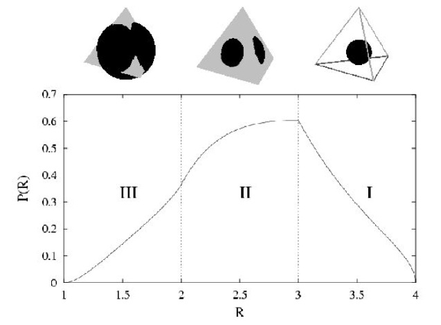
Figure 14.10: Probability (density) distribution of stated $\rho$ generated according to the measure (14.110). The three regions described in the text are also shown.

• region I: $r\in[0,h_{1}]$ ($R\in[4,3]$), where $h_{1}\equiv h_{c}={1\over 4}\sqrt{2\over{3}}$ is the radius of a sphere tangent to the faces of the tetrahedron $T_{\Delta}$. In this case the sphere $\Sigma_{r}$ lies completely within the tetrahedron $T_{\Delta}$. Therefore we only need to generate at random points over its surface. The cartesian coordinates for the sphere are given by

  $$x_{1} = r\,\sin\theta\,\cos\phi$$

  $$x_{2} = r\,\sin\theta\,\sin\phi$$

  $$x_{3} = r\,\cos\theta,$$ (14.115)

  Denoting rand_u() a random number uniformly distributed between 0 an 1, the random numbers $\phi=2\pi$rand_u() and $\theta=\arccos(2$rand_u()$-1)$ (its probability distribution being $P(\theta)=\frac{1}{2}\sin(\theta)$) define an arbitrary state $\rho$ on the surface inside $T_{\Delta}$. The angle $\theta$ is defined between the centre of the tetrahedron (the origin) and the vector ${\bf r_{4}}$, and any point aligned with the origin. Substitution of ${\bf r}=(x_{1},x_{2},x_{3})$ in (14.112) provides us with the eigenvalues $\{$$\lambda_{i}$$\}$ of $\rho$, with the desired $R$ as prescribed by the relationship (14.114). With the subsequent application of the unitary matrices $U$ we obtain a random state $\rho=UD(\Delta)U^{{\dagger}}$ distributed according to the usual measure $\nu=\mu\times{\cal L}_{N-1}$.

• region II: $r\in[h_{1},h_{2}]$ ($R\in[3,2]$), where $h_{2}\equiv\sqrt{h^{2}_{c}+(\frac{D}{2})^{2}}={\sqrt{2}\over 4}$ denotes the radius of a sphere which is tangent to the sides of the tetrahedron $T_{\Delta}$. Contrary to the previous case, part of the surface of the sphere lies outside the tetrahedron. This fact means that we are able to still generate the states $\rho$ as before, provided we reject those ones with negative weights $\lambda_{i}$.

• region III: $r\in[h_{2},h_{3}]$ ($R\in[2,1]$), where $h_{3}\equiv\sqrt{h^{2}_{c}+D^{2}}={\sqrt{6}\over 4}$ is the radius of a sphere passing through the vertices of $T_{\Delta}$. The generation of states is a bit more involved in this case. Again $\phi=2\pi$rand_u(), but the available angles $\theta$ now range from $\theta_{c}(r)$ to $\pi$. It can be shown that $w\equiv\cos(\theta_{c})$ results from solving the equation $3r^{2}w^{2}-\sqrt{\frac{3}{2}}rw+\frac{3}{8}-2r^{2}=0$. Thus, $\theta(r)=\arccos(w(r))$, with $w(r)=\cos\theta_{c}(r)+(1-\cos\theta_{c}(r))$rand_u(). Some states may be unacceptable ($\lambda_{i}<0$) still, but the vast majority are accepted.

Combining these three previous regions, we are able to generate arbitrary mixed states $\rho$ endowed with a given participation ratio $R$.

CURRICULUM VITAE

Personal Data

Name: Josep Batle-Vallespir

D.N.I.: 43.101.564-R

Birthdate: June 8 1976

Birthplace: Sa Pobla, Mallorca

Academic Data

Master Degree in Physics, University of Balearic Islands (1994-1998)

University Professor Assistant, 2000-2001. Subject “Fonaments Físics de l’Enginyeria”, Enginyeria Tècnica Industrial especialitat Electrònica. University of Balearic Islands

PhD Student in Physics under FEDER funding (European Union), 2001-2002

PhD Student in Physics under grant by the Conselleria d’Innovació i Energia, Government of Balearic Islands, 2002-2005

High School Professor of Mathematics, 2005-

University of Balearic Islands

Physics Department

Mateu Orfila building

Carretera de Valldemossa, km 7.5

E-07122, Palma de Mallorca

Fax: +34 971173426

E-mail: vdfsjbv4@uib.es

Publications

• J. Batle, M. Casas, A. Plastino, and A. R. Plastino, On the Connection Between Entanglement and the Speed of Quantum Evolution, Physical Review A 72, 032337 (2005).

• J. Batle, M. Casas, A. Plastino, and A. R. Plastino, Werner States and the Two-Spinors Heisenberg Anti-ferromagnet, Physics Letters A 343, 12 (2005).

• J. Batle, A. R. Plastino, M. Casas, and A. Plastino, Maximally Entangled Mixed States and Conditional Entropies, Physical Review A 71, 024301 (2005).

• J. Batle, A. R. Plastino, M. Casas, and A. Plastino, Some Statistical Features of the Entanglement Changes Associated with Quantum Logical Gates, Physica A 356, 385 (2005).

• J. Batle, M. Casas, A. Plastino, and A. R. Plastino, Entanglement Distribution and Entangling Power of Quantum Gates, Optics and Spectroscopy 99, 371 (2005).

• J. Batle, M. Casas, A. R. Plastino, and A. Plastino, Quantum Entropies and Entanglement, International Journal of Quantum Information 3, 99 (2005).

• J. Batle, M. Casas, A. Plastino, and A. R. Plastino, Metrics, Entanglement, and Mixedness in the Space of Two-qubits, Physics Letters A (2006), in press.

• J. Batle, A. R. Plastino, M. Casas, and A. Plastino, Inclusion Relations Among Separability Criteria, Journal of Physics A 37, 895 (2004).

• J. Batle, A. R. Plastino, M. Casas, and A. Plastino, Some Features of the Conditional q-Entropies of Composite Quantum Systems, European Physical Journal B 35, 391 (2003).

• J. Batle, M. Casas, A. Plastino and A. R. Plastino, On the Correlations Between Quantum Entanglement and q-Information Measures, Physics Letters A 318, 506 (2003).

• J. Batle, M. Casas, A. Plastino, and A. R. Plastino, The Statistics of the Entanglement Generated by the Hadamard-CNOT Quantum Circuit, Physica A 327, 140 (2003).

• J. Batle, M. Casas, M. de Llano, M. Fortes, and F. J. Sevilla, Generalized BCS-BOSE Crossover Picture of Superconductivity, International Journal of Modern Physics B 17, 3271 (2003).

• J. Batle, A. R. Plastino, M. Casas, and A. Plastino, Understanding Quantum Entanglement: Qubits, Rebits and the Quaternionic Approach, Optics and Spectroscopy 94, 700 (2003).

• J. Batle, A. R. Plastino, M. Casas, and A. Plastino, On the Distribution of Entanglement Changes Produced by Unitary Operations, Physics Letters A 307, 253 (2003).

• J. Batle, A. R. Plastino, M. Casas, and A. Plastino, Conditional q-Entropies and Quantum Separability: a Numerical Exploration, Journal of Physics A 35, 10311 (2002).

• J. Batle, M. Casas, A. R. Plastino and A. Plastino, Inference Schemes and Entanglement Determination, Physical Review A 65, 024304 (2002); 65, 049902 (2002).

• J. Batle, A. R. Plastino, M. Casas, and A. Plastino, On the Entanglement Properties of Two Rebits Systems, Physics Letters A 298, 301 (2002).

• J. Batle, M. Casas, A. R. Plastino, and A. Plastino, Entanglement, Mixedness and q-Entropies, Physics Letters A 296, 251 (2002).

• J. Batle, A. R. Plastino, M. Casas and A. Plastino, Quantum Evolution of Power-law Mixed States, Physica A 308, 233 (2002).

• J. Batle, M. Casas, M. Fortes, M. de Llano, and V. V. Tolmachev, Generalizing BCS for Exotic Superconductors, Journal of Superconductivity 15, 655 (2002).

• J. Batle, M. Casas, A. R. Plastino, and A. Plastino, Supersymmetry and the q-Maxent Treatment, Physica A 305, 316 (2002).

• J. Batle, M. Casas, A. R. Plastino, and A. Plastino, On the “Fake” Inferred Entanglement Associated with the Maximum Entropy Inference of Quantum States, Journal of Physics A 34, 6443 (2001).

• J. Batle, M. Casas, M. Fortes, M. A. Solís, M. de Llano, A. A. Valladares, and O. Rojo, Bose-Einstein Condensation of Nonzero-Center-of-Mass-Momentum Cooper Pairs, Physica C 364-365, 161 (2001).

• J. Batle, M. Casas, A. R. Plastino, and A. Plastino, Tsallis Based Variational Method for Finding Approximate Wave Functions, Physica A 294, 165 (2001).

Book Chapters

M. Casas, A. R. Plastino, A. Plastino, and J. Batle,
Approximate density matrices for metal clusters and entangled states,
Condensed Matter Theories Vol. 16, Nova (New York) ed. S. Hernández (2001).

J. Batle, M. Casas, A. R. Plastino, and A. Plastino,
Inference of quantum states: Maximum entropy and fake inferred entanglement,
AIP Proceedings Maxent 2001, Baltimore (USA), ed. R. Fry (2001).

J. Batle, M. Casas, A. Plastino, and A. R. Plastino,
A Survey of Entanglement Changes Associated with Quantum Gates Acting on Two-Qubits,
Trends in Quantum Physics, Nova (New York) eds. V. Krasnoholovets and F. Columbus (2004).

M. Casas, J. Batle, A. Plastino, and A. R. Plastino,
A Systematic Numerical Survey of the Separability Criteria for Bipartite Quantum Systems,
Condensed Matter Theories Vol. 19, Nova (New York) eds. M. Belkacem and P. M. Dinh (2005).

Communications & Posters

J. Batle, M. Casas, A. R. Plastino and A. Plastino,
Inference of quantum states: Maximum entropy and fake inferred entanglement.
“$21^{ST}$ International Workshop on Bayesian Inference and Maximum Entropy Methods in Science and Engineering (MAXENT 2001)”, Johns Hopkins University, Baltimore (USA), 4-9 August 2001.
Oral presentation (30 min).

J. Batle, M. Casas, A. R. Plastino and A. Plastino,
Entanglement, maximum entropy and separability criteria.
Reunión Anual Grupo Especializado de Física Nuclear, Universitat de València, 22-23 February 2002.
Oral presentation (15 min).

J. Batle, M. Casas, A. R. Plastino and A. Plastino,
Maximum entropy and fake inferred entanglement.
“Second European Summer School on Microscopic Quantum Many-Body Theories and Their Applications”, the Abdus Salam International Centre for Theoretical Physics (Miramare-Trieste, Italy), 3-14 September 2001.
Poster presentation.

J. Batle, A. R. Plastino, M. Casas and A. Plastino,
Understanding quantum entanglement: qubits, rebits and the quaternionic approach.
“IX International Conference on Quantum Optics”, Raubichi, Belarus, 14-17 May 2002.
Oral presentation as invited speaker (20 min).

J. Batle, M. Casas, A. Plastino and A. R. Plastino,
On the Correlations Between Quantum Entanglement and q-Information Measures.
“36th Course of the International School of Quantum Electronics on Advances in quantum Information Processing: From Theory to Experiment”, Erice, Sicily, 15-22 March 2003.
Poster presentation.

J. Batle, A. R. Plastino, M. Casas, and A. Plastino,
Spectral decomposition based separability criteria: a numerical survey.
Centennial Anniversary of the Spanish Royal Society of Physics and Chemistry, Grupo expecializado en Información Cuántica (SQUIN), July 2003.
Oral presentation (30 min).

J. Batle, A. R. Plastino, M. Casas, and A. Plastino,
Spectral decomposition based separability criteria: a numerical survey.
4th European QIPC Workshop, Oxford, United Kingdom, July 13-17 2003.
Poster presentation.

J. Batle, M. Casas, A. R. Plastino and A. Plastino,
Quantum Entropies and Entanglement.
“International Meeting on Quantum Information Science”, University of Camerino, Camerino, Italy, 22-19 April 2004.
Poster presentation.

J. Batle, M. Casas, A. Plastino, and A. R. Plastino,
Entanglement Distribution and Entangling Power of Quantum Gates.
“X International Conferece on Quantum Optics ICQO 2004”, Minsk, Belarus, May 30 - June 4.
Oral presentation as invited speaker (30 min).

Courses, Meetings & Workshops

JUAS 2000 (Joint Universities Accelerator School) courses on “Accelerator Physics and Applications”, sponsored by ESI (European Scientific Institute) and organized by several european universities in collaboration with CERN. Archamps (France), and Geneva (Switzerland), January - March 2000.

Participation in the “Workshop on Quantum Information and Quantum Computation”, held at the Abdus Salam International Centre for Theoretical Physics (Miramare-Trieste, Italy), from 14 to 25 October 2002.

Participation in the “Joint ICTP-INFM School-Workshop on Entanglement at the Nanoscale”, held at the Abdus Salam International Centre for Theoretical Physics (Miramare-Trieste, Italy), from October 28 to November 8 2002.

Participation in the course ”Información y Computación Cuánticas”, delivered by Prof. Ignacio Cirac, held at the Theoretical Physics Department of the Universidad Autónoma de Madrid, February 2-6 2004.

Visits to Other Institutions

Collaboration, under the supervision of Prof. G. Ortiz, in the Theoretical (T-11) Division of Los Alamos National Laboratory, New Mexico, USA, regarding the issue of Entanglement and Quantum Phase Transitions, from September to December 2003.

Current Research Interests

The characterization of multipartite entangled states has not been by far completely achieved. This description of entanglement, in the orthodox view of Hilbet space partitioning, offers an arena where the application of the so called entropic inequalities could be of some relevance. Therefore the study of entanglement in multipartite quantum systems plays a paramount role in our current research interest.

Other aspects of quantum entanglement, such as its connection with speed of the quantum evolution of a quantum state, among many other aspects of quantum mechanics, are also under study.

In a more recent status, the characterization of the dynamics of entanglement in quantum phase transitions is a subject that focuses our immediate attention.

References

- [1] A. Einstein, B. Podolsky and N. Rosen, Phys. Rev. 47, 777 (1935).
- [2] E. Schrödinger, Naturwissenschaften 23, 807 (1935). English translation available in Proc. Am. Philos. Soc. 124, 323 (1980).
- [3] J.S. Bell, Physics (Long Island City, N.Y.) 1, 195 (1964).
- [4] J.S. Bell, Speakable and Unspeakable in Quantum Mechanics (Cambridge University Press, Cambridge, UK, 1993).
- [5] S. Kullback, Information Theory and Statistics, (Dover Publications, New York, 1997).
- [6] A. M. Turing, Proc. Lond. Math. Soc. Ser. 2 42, 230 (1936).
- [7] A. I. Khinchin, Mathematical Foundations of Information Theory (Dover Publications, New York, 1957).
- [8] R. Balian, From Microphysics to Macrophysics (Springer, Berlin, 1991).
- [9] V. Buzek, G. Adam, and G. Drobny, Ann. Phys. (N.Y.) 245, 36 (1996).
- [10] E. T. Jaynes, Phys. Rev. 106, 620 (1957); ibid 108, 171 (1957).
- [11] D. ter Haar, Rev. Mod. Phys. 27, 289 (1955).
- [12] A. Galindo and M. A. Martín-Delgado, Rev. Mod. Phys. 74, 347 (2002).
- [13] C. H. Bennett, IBM Jl Res. Dev. 17, 525 (1973).
- [14] C. H. Bennett, Int. Jl of Theor. Phys. 21, 905 (1982).
- [15] R. Landauer, IBM Jl Res. Dev. 5, 183 (1961).
- [16] L. Szilard, Zeitschrift für Physik, 53, 840 (1929).
- [17] J. von Neumann, Mathematische Grundlagen der Quantenmechanik (Springer, Berlin, 1932).
- [18] L. Brillouin, Science and Information Theory (Academic Press, New York, 1956).
- [19] W. H. Zurek, in Frontiers of Nonequilibrium Statistical Physics, G. T. Moore and M. O. Scully, eds. (Plenum Press, New York, 1984).
- [20] V. Vedral, Proc. Roy. Soc. Lond. 456, 969 (1996).
- [21] M. B. Plenio, Phys. Lett. A, 263(4), 281 (1999).
- [22] A. S. Holevo, Problems of Information Transmission 9, 3 (1973).
- [23] R. P. Feynman, The Character of Physical Law (MIT Press, Cambridge, Mass., 1965).
- [24] A. Messiah, Quantum Mechanics (North-Holland, Amsterdam, 1961).
- [25] B. L. van der Waerden, Sources of quatum mechanics (North-Holland, Amsterdam, 1967).
- [26] H. Everett, Rev. Mod. Phys. 29, 454 (1957).
- [27] C. Fuchs and A. Peres, Physics Today, March 2000.
- [28] R. Penrose, Gravity and State Vector Reduction, in Quantum Concepts in Space and Time. Eds. R. Penrose and C. J. Isham (Clarendon Press, Oxford, 1986).
- [29] J. A. Wheeler and W. H. Zurek, Quantum Theory and Measurement (Princeton University Press, Princeton, 1983).
- [30] R. Omnès, Understanding Quantum Mechanics (Princeton University Press, Princeton, 1999).
- [31] C. Cohen-Tannoudji, B. Liu, and F. Laloë, Quantum Mechanics (Wiley, New York, 1977).
- [32] G. W. Mackey, The mathematical foundations of quantum mechanics (Dover, New York, 2004).
- [33] S. L. Adler, Quaternionic Quantum Mechanics and Quantum Fields (Oxford Univ. Press, New York, 1995).
- [34] M. A. Nielsen and I. L. Chuang, Quantum Computation and Quantum Information (Cambridge University Press, Cambridge, 2000).
- [35] L. D. Landau, Z. Phys. 45, 430 (1927).
- [36] D. Bohm and Y. Aharonov, Phys. Rev. 108, 1070 (1957).
- [37] A. Peres and D. R. Terno, Rev. Mod. Phys. 76, 93 (2004).
- [38] S. Weinberg, The Quantum Theory of Fields, Vol. I (Cambridge University Press, Cambridge, UK, 1995).
- [39] J. F. Clauser, M. A. Horne, A. Shimony and R. A. Holt, Phys. Rev. Lett. 23, 880 (1969).
- [40] A. Aspect et al., Phys. Rev. Lett. 47, 460 (1981); ibid. 49, 91 (1982); ibid. 49, 1804 (1982).
- [41] E. Santos, Phys. Rev. Lett. 66, 1388 (1991).
- [42] R. F. Werner, Phys. Rev. A 40, 4277 (1989).
- [43] G. Major, The Quantum Beat: The Physical Principles of Atomic Clocks (Springer, New York, 1998).
- [44] R. Jozsa, D. S. Abrams, J. P. Dowling, and C. P. Williams, Phys. Rev. Lett. 85, 2010 (2000).
- [45] V. Giovanetti, S. Lloyd, and L. Maccone, Europhys. Lett. 62, 615 (2003).
- [46] E. Bagan, M. Baig, and R. Munoz-Tapia, Phys. Rev. Lett. 87, 257903 (2001).
- [47] E. Bagan, M. Baig, and R. Munoz-Tapia, Phys. Rev. A 69, 050303 (2004).
- [48] M. Schlosshauer, Rev. Mod. Phys. 76, 1267 (2004).
- [49] J. Zaanen et al., Phys. Rev. Lett. 94, 230401 (2005).
- [50] J. Friedman et al., Nature 406, 43 (2000).
- [51] J. J. Sakurai, Modern Quantum Mechanics (Addison-Wesley, New York, 1985).
- [52] A. Wehrl, Rev. Mod. Phys. 50, 221 (1978).
- [53] R. Schumacher, Phys. Rev. A 51, 2738 (1995).
- [54] J. S. Dehesa, A. Martinez-Finkelshtein, and V. N. Sorokin, Phys. Rev. A 66, 062109 (2002).
- [55] V. Buyarov, J. S. Dehesa, A. Martinez-Finkelshtein, and Sanchez-Lara, SIAM J. of Sci. Comput. 26, 488 (2004).
- [56] C. Brukner and A. Zeilinger, Phys. Rev. Lett. 83, 3354 (1998).
- [57] C. Brukner and A. Zeilinger, Phys. Rev. A 63, 022113 (2001).
- [58] F. Giraldi and P. Grigolini, Phys. Rev. A 64, 032310 (2001).
- [59] J. D. Bekenstein, Physics Today 33, 24 (1980).
- [60] D. Deutsch, Proc. R. Soc. Lond. A, 400, 97 (1985).
- [61] P. A. Benioff, Int. J. theor. Phys. 21, 177 (1982).
- [62] R. P. Feynman, Int. J. theor. Phys. 21, 467 (1982).
- [63] D. Z. Albert, Phys. Lett. A 98, 249 (1983).
- [64] A. M. Steane, Phys. Rev. A 68, 042322 (2003).
- [65] D. Deutsch, A. Barenco, and A. Ekert, Proc. R. Soc. Lond. A 449, 669 (1995).
- [66] A. Barenco, Proc. R. Soc. Lond. A 449, 679 (1995).
- [67] D. Deutsch and R. Jozsa, Proc. R. Soc. London A 439, 553 (1992).
- [68] D. R. Simon, 1994, Proceedings of the 35th Annual IEEE Symposium on the Foundations of Computer Science (IEEE Computer Society, Los Alamitos, CA), extended abstract p. 116. Full version, in SIAM J. Comput. 26, 1474 (1997).
- [69] L. K. Grover, Proceedings of the 28th Annual ACM Symposium on the Theory of Computing, Philadelphia, PA (Association for Computing Machinery, New York), 212 (1996).
- [70] L. K. Grover, Phys. Rev. Lett. 79, 325 (1997).
- [71] P. W. Shor, Proceedings of the 35th Annual Symposium on the Foundations of Computer Science (IEEE Computer Society Press, Los Alamitos, CA, 1994), 124 (1994).
- [72] A. Ekert and R. Jozsa, Rev. Mod. Phys. 68, 773 (1996).
- [73] H. E. Brandt, Progress in Quantum Electronics 22, 257 (1998).
- [74] L. M. K. Vandersypen ans I. L. Chuang, Rev. Mod. Phys. 76, 1037 (2004).
- [75] M. B. Plenio and P. L. Knight, Physical Review A 53 2986, (1996).
- [76] P. W. Shor, Phys. Rev. A 52, 2493 (1995).
- [77] A. Steane, Rep. Prog. Phys. 61, 117 (1998).
- [78] M. S. Byrd, Lian-Ao Wu, and D. A. Lidar, J. Mod. Opt. 51, 2449 (2004).
- [79] D. A. Lidar and K. B. Whaley, Irreversible Quantum Dynamics (Springer-Verlag, Berlin, 2003).
- [80] D. P. DiVincenzo, Fortschr. Phys. 48, 9 (2000).
- [81] J. I. Cirac and P. Zoller, Phys. Rev. Lett. 74, 4091 (1995); C. Monroe et al., Phys. Rev. Lett. 75, 4714 (1995).
- [82] Q. A. Turchette et al., Phys. Rev. Lett. 75, 4710 (1995)
- [83] H. J. Kimble, Physica Scripta T76, 127 (1998).
- [84] D. Cory et al., Proc. Nat. Acad. Sci. 94, 1634 (1997); N. Gershenfeld and I. Chuang, Science 275, 350 (1997).
- [85] A. Shnirman et al., Phys. Rev. Lett. 79, 2371 (1997); J. E. Mooij et al., Science 285, 1036 (1999).
- [86] D. Loss and D. P. DiVincenzo, Phys. Rev. A 57, 120 (1998).
- [87] The Physics of Quantum Information, edited by D. Bouwmeester, A. Ekert, and A. Zeilinger (Springer-Verlag, Berlin, 2000).
- [88] M. V. Berry, Proc. R. Soc. London A 392, 45 (1984).
- [89] P. Zanardi and M. Rasetti, Phys. Lett. A 264, 94 (1999).
- [90] L. M. Duan and G. Guo, Phys. Lett. A 261, 139 (1999).
- [91] J. Pachos, P. Zanardi, and M. Rasetti, Phys. Rev. A 61, 010305(R) (2000).
- [92] L. M. Duan, J. I. Cirac, and P. Zoller, Science 292, 1695 (2001).
- [93] W.S. Warren, Science 277, 1688 (1997).
- [94] N. Linden and S. Popescu, Phys. Rev. A 59, 137 (1999).
- [95] R. Schack and C. M. Caves, J. Mod. Opt. 47, 387 (2000).
- [96] C. Monroe, D. M. Meekhof, B. E. King, W. M. Itano, and D. J. Wineland, Phys. Rev. Lett 75, 4714 (1995).
- [97] I. Bloch, Physics World, April 2004.
- [98] D. Jaksch et al., Phys. Rev. Lett. 82, 1975 (1999).
- [99] C. H. Bennett and S. J. Wiesner, Phys. Rev. Lett. 69, 2881 (1993).
- [100] K. Mattle, H. Weinfurter, P. G. Kwiat, and A. Zeilinger, Phys. Rev. Lett. 76, 46564659 (1996).
- [101] P. Hausladen, R. Jozsa, B. Schumacher, M. Westmoreland, and W. K. Wootters, Phys. Rev. A 54, 1869 (1996).
- [102] C.H. Bennett, G. Brassard, C. Crepeau, R. Jozsa, A. Peres and W. K. Wootters, Phys. Rev. Lett. 70, 1895 (1993).
- [103] D. Boschi, S. Branca, F. D. Martini, L. Hardy, and S. Popescu, Phys. Rev. Lett. 80, 1121 (1998).
- [104] D. Bouwmeester, J. W. Pan, K. Mattle, M. Eibl, H. Weinfurter, and A. Zeilinger, Nature 390, 575 (1997).
- [105] M. A. Nielsen, E. Knill, and R. Laflamme, Nature 396, 52 (1998).
- [106] M. Riebe, H. Häffner, C. F. Roos, W. Hänsel, J. Benhelm, G. P. T. Lancaster, T. W. Körber, C. Becher, F. Schmidt-Kaler, D. F. V. James and R. Blatt, Nature 429, 734 (2004).
- [107] M. D. Barrett, J. Chiaverini, T. Schaetz, J. Britton, W. M. Itano, J. D. Jost, E. Knill, C. Langer, D. Leibfried, R. Ozeri and D. J. Wineland, Nature 429, 737 (2004).
- [108] S. L. Braunstein, C. A. Fuchs, and H. J. Kimble, J. of Mod. Opt., 47, 267 (2000).
- [109] R. L. Rivest, A. Shamir, and L. M. Adleman, Comm. ACM 21, 120 (1978).
- [110] Hoi-Kwong Lo, S. Popescu and T. Spiller (Editors), Introduction to Quantum Computation and Information (World Scientific, River-Edge, 1998).
- [111] C. H. Bennett and G. Brassard, Proceedings of IEEE International Conference on Computers, Systems and Signal Processing (IEEE, New York, 1984).
- [112] W. K. Wootters and W. H. Zurek, Nature 299, 802 (1982).
- [113] W. Dür, H.-J. Briegel, J. I. Cirac, and P. Zoller, Phys. Rev. A 59, 169 (1999); ibid. 60, 729 (1999).
- [114] C. P. Williams and S.H. Clearwater, Explorations in Quantum Computing (Springer, New York, 1997).
- [115] C. P. Williams (Editor), Quantum Computing and Quantum Communications (Springer, Berlin, 1998).
- [116] A. Ekert, Phys. Rev. Lett. 67, 661 (1991).
- [117] G. P. Berman, G. D. Doolen, R. Mainieri, and V. I. Tsifrinovich, Introduction to Quantum Computers (World Scientific, Sinagapore, 1998).
- [118] B. M. Terhal, Theor. Comp. Sci. 287, 313 (2002).
- [119] A. Peres, Quantum Theory: Concepts and Methods (Kluwer, Dordrecht, 1993).
- [120] M. Horodecki, P. Horodecki and R. Horodecki, Phys. Rev. Lett. 78, 574 (1997).
- [121] M. Horodecki and P. Horodecki, Phys. Rev. A 59, 4206 (1999)
- [122] P. Horodecki, M. Lewenstein, G. Vidal and I. Cirac, Phys. Rev. A 62, 032310 (2000).
- [123] A. Peres, Phys. Rev. Lett. 77, 1413 (1996).
- [124] M. Horodecki, P. Horodecki, and R. Horodecki, Phys. Lett. A 223, 1 (1996).
- [125] T. Hiroshima, Phys. Rev. Lett. 91, 057902 (2003).
- [126] M. A. Nielsen and J. Kempe, Phys. Rev. Lett. 86, 5184 (2001).
- [127] K. G. H. Vollbrecht and M. M. Wolf, J. Math. Phys. 43, 4299 (2002).
- [128] R. Horodecki, P. Horodecki, M. Horodecki, Phys. Lett. A 210, 377 (1996).
- [129] R. Horodecki, M. Horodecki, Phys. Rev. A 54, 1838 (1996).
- [130] N. Cerf, C. Adami Phys. Rev. Lett. 79, 5194 (1997).
- [131] A. Vidiella-Barranco, Phys. Lett. A 260, 335 (1999).
- [132] C. Tsallis, S. Lloyd, M. Baranger, Phys. Rev. A 63, 042104 (2001).
- [133] C. Tsallis, P.W. Lamberti, D. Prato, Physica A 295, 158 (2001).
- [134] S. Abe, Phys. Rev. A 65, 052323 (2002).
- [135] C. Beck and F. Schlogl, Thermodynamics of Chaotic Systems (Cambridge University Press, Cambridge, 1993).
- [136] C. Tsallis, J. Stat. Phys. 52, 479 (1988).
- [137] P. T. Landsberg and V. Vedral, Phys. Lett. A 247, 211 (1998).
- [138] J. A. S. Lima, R. Silva, and A. R. Plastino, Phys. Rev. Lett. 86, 2938 (2001).
- [139] J. Batle, A R Plastino, M. Casas and A. Plastino, J. Phys. A 37, 895 (2004).
- [140] G. Alber, T. Beth, P. Horodecki, R. Horodecki, M. Röttler, H. Weinfurter, R. Werner, A. Zeilinger, Quantum Information, Springer Tracts in Modern Physics 173 (Springer, Berlin, 2001).
- [141] A. Jamiolkowski, Rep. Math. Phys. 3, 275 (1972).
- [142] S. Banach, Théorie des Opérations Linéares, Warsaw, 1932.
- [143] K. Eckert, O. Gühne, F. Hulpke, P. Hyllus, J. Korbicz, J. Mompart, D. Bruß, M. Lewenstein and A. Sanpera, Quantum Information Processing, Gerd Leuchs, Thomas Beth (Eds) Wiley-VCH, Verlag GmbH 2003.
- [144] A. Chefles, C. R. Gilson, and S. M. Barnett, Phys. Lett. A 273, 10 (2000).
- [145] P. Zanardi, D. Lidar, and S. Lloyd, Phys. Rev. Lett. 92, 060402 (2004).
- [146] H. Barnum, E. Knill, G. Ortiz, and L. Viola, Phys. Rev. A 68, 032308 (2003).
- [147] H. Barnum, E. Knill, G. Ortiz, R. Somma, and L. Viola, Phys. Rev. Lett. 92, 107902 (2004).
- [148] S. Popescu, Phys. Rev. Lett. 72, 797 (1994).
- [149] S. Popescu, Phys. Rev. Lett. 74, 2619 (1995).
- [150] J. Batle, M. Casas, A. Plastino and A. R. Plastino, Phys. Lett. A 343, 12 (2005).
- [151] D. B. Greenberger, M. Horne, and A. Zeilinger, Bell’s Theorem, Quantum Theory and Conceptions of the Universe, M. Kafatos, ed. (Kluwer Academic, Dordrecht, 1989).
- [152] A. Acín, D. Druß, M. Lewenstein, and A. Sanpera, Phys. Rev. Lett. 87, 040401 (2001).
- [153] C. H. Bennett, D. P. DiVincenzo, Tal Mor, P. W. Shor, J. A. Smolin and B. M. Terhal, Phys. Rev. Lett. 82, 2881 (1999).
- [154] V. Coffman, J Kundu, and W. Wootters, Phys. Rev. A 61 (2000) 052306.
- [155] M. Horodecki, Quantum Information and Computation 1, 3 (2001).
- [156] C. H. Bennett, H. J. Bernstein, S. Popescu, and B. Schumacher, Phys. Rev. A 53, 2046 (1996).
- [157] C. H. Bennett, D. P. DiVicenzo, J. Smolin, and W. K. Wootters, Phys. Rev. A 54, 3824 (1996).
- [158] W. K. Wootters, Phys. Rev. Lett. 80, 2245 (1998).
- [159] P. Rungta, V. Buzek , C. M. Caves, M. Hillery, and G. J. Milburn, Phys. Rev. A 64 042315 (2001).
- [160] F. Mintert, M. Kus, and A. Buchleitner, Phys. Rev. Lett. 92, 167902 (2004).
- [161] G. Vidal and R. Tarrach, Phys. Rev. A 59, 141 (1999).
- [162] S. J. Akhtarshenas and M. A. Jafarizadeh, e-print quant-ph/0211156 v1.
- [163] V. Vedral et al., Phys. Rev. Lett. 78, 2275 (1997).
- [164] S. Kullback and R. A. Leibler, Ann. Math. Stat. 22, 79 (1951).
- [165] J. Batle, M. Casas, A. R. Plastino, and A. Plastino, Int. J. Quant. Inf. 3, 99 (2005).
- [166] V. Vedral and M. Plenio, Phys. Rev. A 57, 1619 (1998).
- [167] Belita Koiller, Xuedong Hu, R. B. Capaz, A. S. Martins, and S. Das Sarma, An. Acad. Bras. Cienc. 77, 201 (2005).
- [168] K. Eckert, J. Schliemann, D. Bruß, and M. Lewenstein, Ann. of Phys. 299, 88 (2002).
- [169] G. Ghirardi, L. Marinatto, and T. Weber, Journal of Statistical Physics 108, 49 (2002).
- [170] Y. Omar, N. Paunkovic, S. Bose, and V. Vedral, Phys. Rev. A 65, 062305 (2002).
- [171] N. Paunkovic, Y. Omar, S. Bose, and V. Vedral, Phys. Rev. Lett. 88, 187903 (2002).
- [172] P. Zanardi, Phys. Rev. A 65, 042101 (2002).
- [173] M. Horodecki, J. Oppenheim, and R. Horodecki, Phys. Rev. Lett. 89, 240403 (2002).
- [174] S. Popescu and D. Rohrlich, Phys. Rev. A 56, R3319 (1997).
- [175] P. Horodecki, R. Horodecki, and M. Horodecki, Act. Phys. Slov. 48, 141 (1998).
- [176] R. Horodecki, M. Horodecki and P. Horodecki, Phys. Rev. A 59, 1799 (1999).
- [177] V. Buzek, G. Drobny, G. Adam, R. Derka and P. L. Knight, J. Mod. Opt. 44, 1607 (1997).
- [178] A. Rigo, A. R. Plastino, A. Plastino and M. Casas, Phys. Lett. A 270, 1 (2000).
- [179] A. K. Rajagopal, Phys. Rev. A 60, 4338 (1999).
- [180] A. Abe and A. K. Rajagopal, Phys. Rev. A 60, 3461 (1999).
- [181] J. M. G. Sancho and S. F. Huelga, Phys. Rev. A 61, 1 (2000).
- [182] T. A. Brun, C. M. Caves and R. Schack, Phys. Rev. A 63, 042309 (2001)
- [183] J. Batle, M Casas, A. R. Plastino and A. Plastino, J. Phys. A 34, 6443 (2001).
- [184] S. L. Braunstein, A. Mann, and M. Revzen, Phys. Rev. Lett. 68, 3259 (1992).
- [185] J. Batle, M. Casas, A. R. Plastino and A. Plastino, Phys. Rev. A 65, 024304 (2002).
- [186] K. Zyczkowski K, P. Horodecki, A. Sanpera and M. Lewenstein, Phys. Rev. A 58, 883 (1998).
- [187] K. Zyczkowski, Phys. Rev. A 60, 3496 (1999).
- [188] K. Zyczkowski and H. J. Sommers, J. Phys. A 34, 7111 (2001).
- [189] W.J. Munro, D.F.V. James, A.G. White, and P.G. Kwiat, Phys. Rev. A 64 (2001) 030302.
- [190] S. Ishizaka and T. Hiroshima, Phys. Rev. A 62, 022310 (2000).
- [191] J. Batle, M. Casas, A. R. Plastino and A. Plastino A, Phys. Lett. A 298, 301 (2002).
- [192] J. Batle, M. Casas, A. R. Plastino and A. Plastino A, Phys. Lett. A 296, 251 (2002).
- [193] M. Horodecki, P. Horodecki and R. Horodecki, Phys. Lett. A 223, 1 (1996).
- [194] J. Batle, A. R. Plastino, M. Casas, and A. Plastino, Eur. Phys. J. B 35, 391 (2003).
- [195] M. Pozniak, K. Zyczkowski and M. Kus, J. Phys A 31, 1059 (1998).
- [196] J. Batle, A. R. Plastino, M. Casas and A. Plastino, J. Phys A 35, 10311 (2002).
- [197] S. L. Braunstein, C. M. Caves, R. Jozsa, N. Linden, S. Popescu and R. Schack, Phys. Rev. Lett. 83, 1054 (1999).
- [198] F. C. Alcaraz and C. Tsallis, Phys. Lett. A 301, 105 (2002).
- [199] C. Tsallis, D. Prato and C. Anteneodo, Eur. Phys. J. B 29, 605 (2002).
- [200] J. Batle, A.R. Plastino, M. Casas, A. Plastino, Phys. Lett. A 307, 253 (2003).
- [201] M. Casas, S. Mart nez, F. Pennini, and A. Plastino, Physica A 305, 41 (2002).
- [202] M. Gell-Mann and C. Tsallis, Nonextensive Entropy - Interdisciplinary Applications (Oxford University Press, Oxford, 2003).
- [203] N. A. Peters, J. B. Altepeter, D. Branning, E. R. Jeffrey, T.-C. Wei, and P. G. Kwiat, Phys. Rev. Lett. 92, 133601 (2004).
- [204] J. Batle, M. Casas, A. Plastino, A. R. Plastino, Phys. Rev. A 71, 024301 (2005).
- [205] J. Batle, M. Casas, A. Plastino, and A. R. Plastino, Phys. Lett. A 318, 506 (2003).
- [206] N. Canosa, R. Rossignoli, Phys. Rev. Lett. 88, 170401 (2002).
- [207] F. Giraldi, P. Gringolini, Phys. Rev. E 64, 2310 (2001).
- [208] K. Zyczkowski and M. Kus, J. Phys. A 27, 4235 (1994).
- [209] V. D. Milman and G. Schechtman, Asymptotic Theory of Finite Dimensional Normed Spaces, Springer Lect. Notes in Math., Vol. 1200, Appendix 3 (2001).
- [210] L. Gurvits and H. Barnum, Phys. Rev. A 66, 062311 (2002).
- [211] D. M. Y. Sommerville, An Introduction to the Geometry of N Dimensions (Dover, New York, 1958).
- [212] J. Batle, M. Casas, A. Plastino, and A. R. Plastino, Metrics, Entanglement, and Mixedness in the Space of Two-qubits, sent to a Physics Letters A (2005).
- [213] P. B. Slater, J. Phys. A 32, 5261 (1999).
- [214] P. B. Slater, Eur. Phys. J. B 17, 471 (2000).
- [215] P. B. Slater, Lett. Math. Phys. 52, 343 (2000).
- [216] P. B. Slater, Quant. Info. Process. 1, 397 (2002).
- [217] M. Hübner, Phys. Lett. A 163, 239 (1992).
- [218] D. J. C. Bures, Trans. Am. Math. Soc. 135 199, (1969).
- [219] K. Zyczkowski and H.-J. Sommers, Phys. Rev. A 71, 032313 (2005).
- [220] R. E. Kass, Statist. Sci. 4, 188 (1989).
- [221] C. M. Caves, C.A. Fuchs, P. Rungta, Found. Phys. Lett. 14 199, (2001).
- [222] E. C. G. Stueckelberg, Helv. Phys. Acta 33, 727 (1960).
- [223] M. Guenin, C. Piron, H. Ruegg, E. C. G. Stueckelberg, Helv. Phys. Acta 34, 675 (1961).
- [224] G. G. Emch, Mathematical and Conceptual Foundations of 20th Century Physics (North-Holland, Amsterdam, 1986).
- [225] W. K. Wootters, J. Math. Phys. 43, 4307 (2002).
- [226] J. Batle, A.R. Plastino, M. Casas and A. Plastino, Optics and Spectroscopy 94, 700 (2003)
- [227] S. P. Brumby and G. C. Joshi, Chaos Sol. and Frac. 7, 747 (1996).
- [228] B. Kraus, J. I. Cirac, Phys. Rev. A 63, 062309 (2001).
- [229] W. Dür, G. Vidal, J. I. Cirac, N. Linden, S. Popescu, Phys. Rev. Lett. 87, 137901 (2001).
- [230] X. Wang, P. Zanardi, Phys. Rev. A 66, 044303 (2002).
- [231] A. Barenco, D. Deutsch, A. Eckert, Phys. Rev. Lett. 74, 4083 (1995).
- [232] A. Barenco, C. H. Bennett, R. Cleve, D. P. DiVicenzo, N. Margolus, P. Shor, T. Sleator, J. A. Smolin and H. Wienfurter, Phys. Rev. A 52, 3457 (1995).
- [233] J. Batle, M. Casas, A. Plastino, and A. R. Plastino, Physica A 327, 140 (2003).
- [234] P. Zanardi, C. Zalka and L. Faoro, Phys. Rev A 62, 030301 (2000).
- [235] H.-J. Sommers and K. Zyczkowski, J. Phys. A 36, 10083 (2003).
- [236] J. Batle, M. Casas, A. Plastino, and A. R. Plastino, Optics and Spectroscopy 99, 371 (2005).
- [237] G. Vidal, K. Hammeter and J.I. Cirac, Phys. Rev. Lett. 88, 237902 (2002).
- [238] J. Batle, M. Casas, A. Plastino, and A. R. Plastino, Physica A 356, 385 (2005).
- [239] J. Batle, A. R. Plastino, M. Casas and A. Plastino. To be published elsewhere.
- [240] V. Giovanetti, S. Lloyd, and L. Maccone, Phys. Rev. A 67, 052109 (2003).
- [241] N. Margolus and L. B. Levitin, Physica D 120, 188 (1998).
- [242] C. M. Caves and P. D. Drummond, Rev. Mod. Phys. 66, 481 (1994).
- [243] S. Lloyd, Nature 406, 1047 (2000).
- [244] J. Batle, M. Casas, A. Plastino and A. R. Plastino, Phys. Rev. A 72, 032337 (2005).
- [245] R. Somma, G. Ortiz, H. Barnum, E. Knill and L. Viola, Phys. Rev. A 70, 042311 (2004).
- [246] M. Nakahara, Geometry, Topology and Physics (Institute of Physics Publishing, Bristol, UK, 2002).
- [247] N. D. Mermin and H. Wagner, Phys. Rev. Lett. 17, 1133 (1966).
- [248] F. J. Wegner, J. Math. Phys. 12, 2259 (1971).
- [249] S. Sachdev, Quantum Phase Transitions (Cambridge University Press, Cambridge, UK, 1999).
- [250] E. Barouch, B. M. McCoy, and M. Dresden, Phys. Rev. A 2, 1075 (1970).
- [251] E. Barouch and B. M. McCoy, Phys. Rev. A 3, 786 (1971).
- [252] T. J. Osborne and M. A. Nielsen, Quantum Inf. Process. 1, 45 (2002); Phys. Rev. A 66, 032110 (2002).
- [253] A. Osterloh, L. Amico, G. Falci, and R. Fazio, Nature (London) 416, 608 (2002).
- [254] M. C. Arnesen, S. Bose, and V. Vedral, Phys. Rev. Lett. 87, 017901 (2001).
- [255] G. Vidal, J. I. Latorre, E. Rico, and A. Kitaev, Phys. Rev. Lett. 90, 227902 (2003).
- [256] F. Verstraete, M. A. Martin-Delgado, and J. I. Cirac, Phys. Rev. Lett. 92, 087201 (2003).
- [257] J. Richter, S. E. Krüger, D. J. J. Farnell, and R. F. Bishop, Series on Advances in Quantum Many-Body Theory, Vol. 5 (World Scientific, 2001), 239.
- [258] K. Okamoto and K. Yasumura, Journal of the Physical Society of Japan 59, 993 (1990).
- [259] A. Fujii, J. Phys. A 30, 6661 (1997).
- [260] R. Somma, G. Ortiz, and J. Batle. To be published elsewhere (2005).
- [261] P. Jordan and E. Wigner, Z. Phys. 47, 631 (1928).
- [262] Aditi Sen(De), Ujjwal Sen, and Maciej Lewenstein, Phys. Rev. A 70, 060304(R) (2004).
- [263] Taken from J. Preskill, The future of quantum information science. Available at http://www.theory.caltech.edu/people/prekill/ph229 (1999).
- [264] P. Horodecki and R. Horodecki, Quantum Information and Computation 1, 45 (2001).
- [265] A. Wong and N. Christensen, Phys. Rev. A 63, 044301 (2001).
- [266] J. Eisert, P. Hyllus, O. Gühne and M. Curty, Phys. Rev. A 70, 062317 (2004).
- [267] T. Tilma, M. Byrd and E. C. G. Sudarshan, J. Phys. A 35, 10445 (2002).
- [268] T. W. B. Kibble, J. Phys. A 9, 1387 (1976); Phys. Rep. 67, 183 (1980).
- [269] W. H. Zurek, Nature (London) 317, 505 (1985); Acta Phys. Pol. B 24, 1301 (1993); Phys. Rep. 276, 177 (1996).
- [270] A. Vilenkin and E. P. S. Shellard, Cosmic Strings and other Topological Defects (Cambridge University Press, Cambridge, 1994), pp. 59.
- [271] A. Haar, Ann. Math. 34, 147 (1933).
- [272] M. L. Mehta, Random Matrices (Academic, New York, 1990).
- [273] J. Conway, Course in Functional Analysis (Springer-Verlag, New York, 1990).
- [274] M. Chaichian and R. Hagedorn, Symmetries in quantum mechanics, (Inst. of Phys. Publ., Bristol).
- [275] A. Hurwitz, Nachr. Ges. Wiss. Gött. Math.-Phys. Kl. 71 (1887).
- [276] V. L. Girko, Theory of Random Determinants (Kluwer, Dordrecht, 1990).