General entanglement scaling laws from time evolution

Abstract

We establish a general scaling law for the entanglement of a large class of ground states and dynamically evolving states of quantum spin chains: we show that the geometric entropy of a distinguished block saturates, and hence follows an entanglement-boundary law. These results apply to any ground state of a gapped model resulting from dynamics generated by a local hamiltonian, as well as, dually, to states that are generated via a sudden quench of an interaction as recently studied in the case of dynamics of quantum phase transitions. We achieve these results by exploiting ideas from quantum information theory and making use of the powerful tools provided by Lieb-Robinson bounds. We also show that there exist noncritical fermionic systems and equivalent spin chains with rapidly decaying interactions whose geometric entropy scales logarithmically with block length. Implications for the classical simulatability are outlined.

At the heart of the intriguing complexity of describing quantum many-body systems is the entanglement contained in the system’s state: if the state is highly entangled, one needs a large number of parameters to describe it classically. The scaling of the geometric entropy [1–11] – the degree of entanglement of a distinguished subsystem with respect to the rest – for quantum many-particle systems, such as those encountered in condensed matter physics, is the crucial parameter which quantifies whether the state is hard or easy to simulate using density-matrix renormalisation group methods [8].

Recently, motivated partially by questions of simulatability, there has been a considerable effort to precisely characterise scaling laws for ground-state entanglement, which we call the static geometric entropy [1–11] Indeed, substantial progress has been made in answering this difficult question: earlier conjectures, for which there was only numerical evidence, could be resolved. For example, it is now known that for gapped bosonic harmonic systems, such as free field models [12], the geometric entropy scales like the boundary area of a distinguished region, and not the volume [6]. The only precise results available at the current time pertain to quasi-free (or Gaussian) bosonic and fermionic models [4, 7, 9] and equivalent 1D spin chains. Apart from integrable systems and matrix-product state hamiltonians (which satisfy an area law by construction [13]), there is a dearth of results concerning static geometric entropy for systems as simple as the 1D spin-1 Heisenberg model. How does the geometric entropy scale for general interacting systems?

There are also very few results available about the strongly related case of geometric entropy for dynamically evolving states [14]. The dynamic geometric entropy occupies centre stage when trying to simulate systems which undergo a sudden quench of a local interaction, for example, when a system is in a Mott phase when the hopping is suddenly altered. In the Mott phase the geometric entropy is zero and grows as the system evolves [14]. It is far from obvious how the geometric entropy should scale as a function of time in these and similar systems dynamically undergoing a quantum phase transition.

In this Letter we establish the first scaling laws for the geometric entropy of a general class of quantum states that goes significantly beyond Gaussian models. On one hand, we will show that if any state of 1D spins whose geometric entropy satisfies a boundary law (i.e., it saturates as a function of $n$, the number of spins) is subjected to dynamics according to an arbitrary 1D local model $K$ for any constant time $t$ then the dynamic geometric entropy will continue to satisfy a boundary law, albeit saturating at a larger constant which depends linearly on $|t|$. On the other hand, when considering the time evolution generated by the local hamiltonian $K$, the state that results from this time evolution can be thought of as the ground state of a gapped hamiltonian, local or with rapidly decaying interactions [15]. All constituents will eventually become correlated, but the entanglement built up between remote parts can be bounded, an intuition that we will cast into a rigourous form. Hence, this reasoning is a device that allows us to establish the result that the static as well as the dynamical geometric entropy of a large class of models, including strongly correlated systems, satisfies a boundary law.

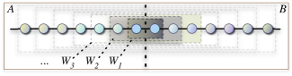
Figure 1: Hierarchy of unitaries $W_{1}(t),W_{2}(t),...$ with exponentially decreasing entangling power over the boundary of $A$ and $B$ .

To actually carry out the argument outlined above we use the powerful machinery of Lieb-Robinson bounds [16, 17, 18, 19]. The intuition we develop is that in a many-body system with local interactions there is a finite speed of sound, and hence a finite velocity of information transfer, resulting from local interactions. The Lieb-Robinson bound is the precise quantification of this statement: it says that the norm of the commutator of two operators, one of which is evolving according to local dynamics, is exponentially small in the separation between the two operators for short times. This inequality allows us to precisely bound the entanglement that can develop across the boundary of a distinguished region for short times. In turn, we find that for large times of the order of the logarithm of the number of spins, the boundary law for the dynamic geometric entropy breaks down. We show this dually by explicitly constructing a local translation-invariant gapped system whose ground state violates an area law.

Geometric entropy in spin chains. – We will, for the sake of clarity, describe our results mainly for a finite chain $\mathcal{C}$ of $n$ distinguishable spin-$1/2$ particles. The family $H$ of local hamiltonians we focus on (which implicitly depends on $n$) is defined by $H=\sum_{j=0}^{n-2}H_{j}$, where $H_{j}$ acts nontrivially only on spins $j$ and $j+1$. We set the energy scale by assuming that $\|H_{j}\|$ scales as a constant with $n$ for all $j=0,1,\ldots,n-1$, where $\|\cdot\|$ denotes the operator norm. The interaction terms $H_{j}$ can, w.l.o.g., be taken to be positive semidefinite, and may depend on time as $H_{j}=H_{j}(t)$.

Consider a bi-partition of the chain into two contiguous blocks $A$ and $B$ of spins of sizes $m=|A|$ and $n-m=|B|$, $m<n$. We will find boundary laws – a saturation of the block entanglement – independent of the system size (we avoid the technicalities arising in the case of infinite systems which might obscure the main point). For simplicity we assume $m<n/2$ and we let $|\psi(t)\rangle=e^{itH}|{0}\rangle$. The initial state is taken to be a product state $|0\rangle$, but the argument is general enough to be applicable for any matrix-product or finitely correlated [20, 8] initial state, or a state resulting from a quantum cellular automata. Consider the Schmidt decomposition

$$|\psi(t)\rangle=\sum_{j=0}^{2^{m}-1}s_{j}^{1/2}(t)|u_{j}(t),v_{j}(t)\rangle,$$

where the $s_{j}(t)$ are the non-increasingly ordered Schmidt coefficients. They are given by the eigenvalues of ${M}(t)={C}(t){C}^{\dagger}(t)$, where $|\psi(t)\rangle=\sum_{j=0}^{2^{m}-1}\sum_{k=0}^{2^{n-m}-1}C_{j,k}(t)|j,k\rangle$, and the $|j\rangle$ and $|k\rangle$ form an orthonormal basis for $\mathcal{H}_{A}$ and $\mathcal{H}_{B}$, respectively. The geometric entropy of a block $A$, or the block entanglement, is given by the von-Neumann entropy $S(m)=-\sum_{j=0}^{2^{m}-1}s_{j}\log_{2}(s_{j})$ [21]. We denote by $H_{A}=\sum_{j=0}^{m-2}H_{j}$ and $H_{B}=\sum_{j=m}^{n-2}H_{j}$ the local parts of the hamiltonian $H$, which act nontrivially only on subsystem $A$ and $B$, whereas $H_{I}=H_{m-1}$ denotes the interaction term.

Entanglement scaling in dynamically evolving quantum states. – In this section we prove an upper bound for the dynamic geometric entropy $S(m)$, $S(m)\leq c_{0}+c_{1}|t|$ , where $c_{0},c_{1}>0$ depend only on $\|h\|$ [22] and not on $n$. Thus, the entropy of the block $A$ scales, asymptotically, less than a constant. Our first step is to obtain the decomposition

$$e^{itH}=(U_{A}(t)\otimes U_{B}(t))V(t).$$

We do this by guessing $U_{A}(t)=e^{itH_{A}}$ and $U_{B}(t)=e^{itH_{B}}$. The idea here is that the dynamics generated by $H$ should be similar to those generated by $H_{A}+H_{B}$ preceded by a unitary $V(t)$ that “patches up” the removed interaction. We obtain a differential equation for $V(t)=e^{-it(H_{A}+H_{B})}e^{itH}=e^{-it(H-H_{I})}e^{itH}$: ${dV(t)}/{dt}=V(t)L(t),$. The “hamiltonian” $L(t)=iH_{I}+\int_{0}^{t}\tau_{u}^{H}([H,H_{I}])\,du$, where $\tau_{t}^{M}(N)=e^{-itM}Ne^{itM}$ for operators $N,M$, is antihermitian, so that the dynamics this integro-differential equation generates is unitary.

Our strategy at this point is to decompose $V(t)$ into a product of strictly local unitary operations [23] $V_{\Lambda_{j}}(t)$ which act nontrivially only on $\Lambda_{j}=\{x:d(x,m)\leq j\}$, which consists of only those sites within a distance $j$ from the boundary. This decomposition for $V(t)$, depicted in Fig. 1, is then

$$V(t)=W_{n-m}(t)W_{n-m-1}(t)\cdots W_{2}(t)W_{1}(t),$$

where $W_{k}(t)=V_{\Lambda_{k}}(t)V_{\Lambda_{k-1}}^{\dagger}(t)$ acts nontrivially only on $\Lambda_{k}$. Also, we set $W_{1}(t)=V_{\Lambda_{1}}(t)$ and $W_{n-m}(t)=V(t)V^{\dagger}_{n-m-1}(t)$. Physically, we expect that the unitary operators $W_{l}(t)$ are successively weaker and weaker. To find a bound on $\|W_{l}(t)-\mathbb{I}\|$ we now invoke the machinery of Lieb-Robinson bounds [16] (see Ref. [19] for a simple direct proof) on the speed of sound in systems evolving according to local dynamics: the strongest available such bound [19] yields

$$\|\tau_{t}^{H_{\Lambda_{l}}}(M)-\tau_{t}^{H_{\Lambda_{l-1}}}(M)\|\leq\delta_{l}|t|^{l}/l!,$$

with $\delta_{l}=\|M\|2^{l}\|h\|^{l}$, where $M=[H_{\Lambda_{k}},H_{I}]$ is the same for all $k$ as long as $k>1$. This is indeed the powerful tool we need to derive the desired bound concerning the deviation from each of the unitaries $W_{l}(t)$ from the identity: it exponentially bounds the information spread in a system undergoing dynamics under a local hamiltonian. We hence find

$$\|W_{l}(t)-\mathbb{I}\|=\|V_{\Lambda_{l}}(t)-V_{\Lambda_{l-1}}(t)\|\leq\delta_{l}|t|^{l+2}/(l+2)!.$$

In the last inequality, we have expressed the operators $V_{\Lambda_{l}}(t)$ as integrals in time [24]. We note that this bound is decaying faster than exponential in $l$. This bound tells us that we can write $W_{l}(t)=\mathbb{I}+\varepsilon_{l}(t)X_{l}(t)$, where $\|X_{l}(t)\|=1$ and $\varepsilon_{l}(t)\leq\min\{2,{\delta_{l}|t|^{l+2}}/{(l+2)!}\}$. Let us now consider the action of $e^{itH}$ on the initial product state vector $|{0}\rangle$,

$$e^{itH}|{0}\rangle=e^{it(H-H_{I})}\prod_{k=1}^{n-m}W_{k}(t)|{0}\rangle.$$

We define $|\psi_{l}(t)\rangle=\prod_{k=1}^{l}W_{k}(t)|{0}\rangle$. Let us now choose $l$ large enough so that this bound for $W_{l}(t)$ is strong enough that $\varepsilon_{l}(t)\leq\min\{2,\|M\|{\delta_{l}|t|^{l+2}}/{(l+2)!}\}$ is small [25]. Then $|\psi_{l}(t)\rangle$ is in a product with respect to the spins outside the region $\Lambda_{l}$ There are, in general, at most $2^{l}$ nonzero Schmidt coefficients for $|\psi_{l}(t)\rangle$ with respect to the bi-partition $AB$. Now we consider the action of $W_{l+1}(t)$ on $|\psi_{l}(t)\rangle$ which yields $|\psi_{l+1}(t)\rangle$. In the computational basis, we have

$$|\psi_{l+1}(t)\rangle=\sum_{j,k=0}^{2^{l+1}-1}\bigl{(}(C_{l})_{j,k}(t)+\varepsilon_{l+1}(t)(D_{l})_{j,k}(t)\bigr{)}|j,k\rangle,$$

setting $|\psi_{l}(t)\rangle=\sum_{j,k=0}^{2^{l+1}-1}(C_{l})_{j,k}(t)|j,k\rangle$ and $X_{l+1}(t)|\psi_{l}(t)\rangle=\sum_{j,k=0}^{2^{l+1}-1}(D_{l})_{j,k}(t)|j,k\rangle$. The normalisation condition and $\|X_{l}(t)\|\leq 1$ imply that $\|{C}_{l}\|\leq 1$ and $\|{D}_{l}\|\leq 1$. We use Weyl’s perturbation theorem [28] to bound the Schmidt coefficients $s^{(l+1)}_{j}$ of $|\psi_{l+1}(t)\rangle$, given by the eigenvalues of $(C_{l}+\varepsilon_{l+1}(t)D_{l})(C_{l}+\varepsilon_{l+1}(t)D_{l})^{\dagger}$. We apply Weyl’s perturbation theorem to the operators ${P}=C_{l}C_{l}^{\dagger}$ and ${Q}=\varepsilon_{l+1}(t)(C_{l}D_{l}^{\dagger}+D_{l}C_{l}^{\dagger})+\varepsilon_{l+1}^{2}(t)D_{l}D_{l}^{\dagger}$ with $\|{Q}\|\leq c\varepsilon_{l+1}(t)$, with $c>0$. The eigenvalues of ${P}$ are precisely the $2^{l}$ Schmidt coefficients of $|\psi_{l}(t)\rangle$. Weyl’s perturbation theorem tells us that the first $2^{l}$ eigenvalues of ${P}+{Q}$ have to be close to the Schmidt coefficients of $|\psi_{l}(t)\rangle$ and the remaining $2^{l}$ eigenvalues have magnitude less than $\varepsilon_{l+1}(t)$ [26]. Exploiting these bounds iteratively, we find that the Schmidt coefficients satisfy the bound $s_{j}(t)\leq\min\{{1}/{2^{\kappa|t|}},2^{\kappa|t|-vj}\}$, for some $\kappa,v>0$. Hence the geometric entropy $S(m)$ satisfies the upper bound $S(m)\leq c_{0}+c_{1}|t|$, where $c_{0},c_{1}>0$. This holds true for all $n$. In other words, we can perform “the limit of infinite system size” $n\rightarrow\infty$. When we let $|t|=\log(n)$ our bounds begin to fall apart: the Lieb-Robinson bound becomes a polynomial bound. This situation can be saturated, see below.

Entropy-boundary laws for approximately local quantum spin systems. – We now show that the entropy-area law for dynamically evolving product states implies entropy-area laws for the ground states of noncritical approximately local quantum spin systems. The product $|{0}\rangle$ is the unique ground state of the hamiltonian $Z=-\sum_{j=0}^{n-1}\sigma^{3}_{j}$. Let $H$ be our hamiltonian. Then $|\psi(t)\rangle$ is the unique ground state of the new hamiltonian $K=e^{itH}Ze^{-itH}$, having exactly the same spectrum as $Z$. Moreover, while $K$ is no longer strictly local in general, it is approximately local with exponentially decaying interactions. The way to see this is to apply a Lieb-Robinson bound to the interaction term $e^{itH}\sigma_{j}^{3}e^{-itH}$: We consider the difference between $e^{itH}\sigma_{j}^{3}e^{-itH}$, having support equal to $\mathcal{C}$, and the strictly local $e^{itH_{\Lambda_{k}(j)}}\sigma_{j}^{3}e^{-itH_{\Lambda_{k}(j)}}$, with ${\Lambda_{k}(j)}=\{x:d(x,j)\leq k\}$, which has support on $2k+1$ sites. This difference can be bounded using the Lieb-Robinson bound, $\|\tau^{H}_{t}(\sigma_{j}^{3})-\tau^{H_{{\Lambda_{k}(j)}}}_{t}(\sigma_{j}^{3})\|\leq ce^{\kappa|t|-vk}$, with $c>0$. Thus, the interaction term $\tau^{H}_{t}(\sigma_{j}^{3})$ couples spins from site $j$ exponentially weakly. What sort of hamiltonians $K=e^{itH}Ze^{-itH}$ – clearly a large class of gapped models – arise in this way? Insight can be provided by the following example: Let $H=\sum_{j}\sigma_{j}^{x}\sigma_{j+1}^{y}$. For small $t$ the hamiltonian $K$ will look like $K=Z+\lambda(t)\sum_{j}\sigma_{j}^{x}\sigma_{j+1}^{x}+\sigma_{j}^{y}\sigma_{j+1}^{y}+O(t^{2})$. In this case $K$ is similar to the $XY$ model in an external magnetic field with small higher order terms. With the inclusion of larger neighborhoods, in turn, local hamiltonians can be approximated to any accuracy. Another useful hamiltonian which can arise in this way is the strictly local cluster hamiltonian [29] (carrying over also to the higher-dimensional case): set $H=\sum_{j}\sigma_{j}^{x}\sigma_{j+1}^{x}$. In this case, when $t=\pi/2$, $K$ is the hamiltonian having the cluster state as a unique ground state.

Logarithmic divergence of geometric entropy of gapped systems. – We now construct an explicit situation where a gapped 1D spin system ${\cal C}$ ndeed violates the entanglement-boundary law. We again consider a family of spin systems, consisting of a block $A$ consisting of $m$ spins, and a block $B$ containing the remaining $n-m$ spins. As before, $S(m)$ is defined to be the geometric entropy of a block $A$ of $m$ spins in the limit of an infinite chain, for simplicity with periodic boundary conditions. By virtue of the familiar Jordan-Wigner transformation [27], we may consider the fermionic model

$$H=\sum_{l,k=0}^{n-1}c_{l}^{\dagger}M_{l-k}c_{k},$$

where $M_{l}\in\mathbb{R}$, $l=0,\ldots,n-1$. The hermiticity of $H$ and the periodic boundary conditions are reflected by the conditions $M_{l}=M_{-l}$ for all $l=0,\ldots,n-1$ and $M_{l}=M_{l+n}$. We can easily map the above hamiltonian onto the one for non-interacting fermions, preserving the anti-commutation relations: $H=\sum_{k=0}^{n-1}\varepsilon_{k}b_{k}^{\dagger}b_{k}$, where $\varepsilon_{k}$, $k=0,\ldots,n-1$, are the eigenvalues of $M$, given by $\varepsilon_{k}=\sum_{j=0}^{n-1}e^{2\pi i(j+1)k/n}M_{j}$. The ground state can then be easily found: it is the state with unit occupancy for each $k$ with $\varepsilon_{k}<0$. If the value $0$ is not contained in the spectrum, this ground state is non-degenerate. We now consider the subsystem $A$. The reduced state $\rho_{m}$ of this block is characterised by the spectrum of the real symmetric $m\times m$ Toeplitz matrix $T_{m}$ [28], which defines the second moments of fermionic operators [4, 30, 9]. The $l$-th row of this matrix is given by $(t_{-l+1},t_{-l+2},...,t_{0},\ldots,t_{m-l})$, where $t_{l}=\sum_{k=0}^{n-1}e^{-ilk}{\varepsilon_{k}}/{(n|\varepsilon_{k}|)}$. At this point, we may take the limit $n\rightarrow\infty$, for fixed $m$, and consider long-ranged interactions, and hence sequences of couplings $\{M_{l}\}_{l\in\mathbb{N}},\,M_{l}\in\mathbb{R}$. This means that in the continuum limit, we can consider functions $\phi:(0,2\pi]\rightarrow\mathbb{R}$, representing the spectrum of the interaction matrix, and $t_{l}={1}/({2\pi})\int_{0}^{2\pi}e^{-ilx}{\phi(x)}/{|\phi(x)|}dx$. We can now make use of a very useful bound of Ref. [9], stating that $S(m)\geq-(\log_{2}|\det[T_{m}]|)/2$. Hence, to show that $S(m)=\Omega(\log m)$, we have to bound the Toeplitz determinant $\det[T_{m}]$. This we can do using a proven instance of the Fisher-Hartwig conjecture [30, 31], determining the scaling of the determinants of Toeplitz matrices. Using these ideas, we are now construct a model with the mentioned surprising properties: We take the interactions $M_{k}=\int_{0}^{2\pi}\phi(x)e^{-ixk}/(2\pi)$ to be given by $M_{k}=-i(e^{ik\pi/2}-1)^{3}(1+e^{i\pi k/2})/(2e^{2\pi ik}k\pi)$, so a $1/k$ decay of the interactions, as in case of an unshielded Coulomb interaction. This gives rise to the Fourier transform $\phi$ that takes the value $1$ in $x\in(0,\pi/2]$, and $(3\pi/2,2\pi]$ and the value $-1$ in $x\in(\pi/2,3\pi/2]$. In this setting, the proven instance of the Fisher-Hartwig conjecture then indeed allows us to argue that $|\det[T_{m}]|=\Omega(\log m)$ [31]. This hamiltonian is obviously gapped: the quasi-particle excitation spectrum is even constant, and never crosses zero, so it defines a gapped system. Still, we find a logarithmically divergent geometric entropy. This is an example of a ground state that is not covered by the above statement for small times.

Outlook. – In this work we have introduced an approach to assess geometric entropies in many-body systems. We have found that many ground states of quasi-local gapped hamiltonians, while being far from quasi-free, still exhibit a saturating geometric entanglement, and hence an entanglement-area law. The studied gapped systems are rigorously classically efficiently simulatable: one can obtain all expectation values of local observables with polynomial computational resources [17]. Simulatability is closely linked with 1D entropy boundary laws [8]. This connection is even more direct in our case because matrix-product states which faithfully approximate our ground states can be explicitly constructed [18]. Such efficient descriptions in terms of matrix-product states would also be generated by an eventually successful application of the DMRG algorithm to our systems.

Two-dimensional systems are in principle accessible with the methods introduced here. This method opens up the way toward studying the complexity of gapped many-body systems and the accompanying ground-state entanglement scaling (as well as capacities of quantum channels based on interacting systems [32]). Intriguingly, we finally found an example of a gapped system with a divergent block entanglement, rendering the connection between criticality and validity of an area theorem more complex than anticipated.

Acknowledgements. – We would like to thank M. Cramer for discussions. This work was supported by the DFG (SPP 1116, SPP 1078), the EU (QAP), the QIP-IRC, the Microsoft Research Foundation, and the EURYI Award of JE.

Note added: This work complements the simultaneously submitted Ref. [33].

References

- [1] A. Osterloh, L. Amico, G. Falci, and R. Fazio, Nature 416, 608 (2002); T.J. Osborne and M.A. Nielsen, Phys. Rev. A 66, 032110 (2002).
- [2] K. Audenaert, J. Eisert, M.B. Plenio, and R.F. Werner, Phys. Rev. A 66, 042327 (2002).
- [3] G. Vidal, J.I. Latorre, E. Rico, and A. Kitaev, Phys. Rev. Lett. 90, 227902 (2003); J.I. Latorre, E. Rico, and G. Vidal, Quant. Inf. Comp. 4, 48 (2004).
- [4] M. Fannes, B. Haegeman, and M. Mosonyi, J. Math. Phys. 44, 6005 (2003); A.R. Its, B.-Q. Jin, and V.E. Korepin, J. Phys. A 38, 2975 (2005); J.P. Keating and F. Mezzadri, Phys. Rev. Lett. 94, 050501 (2005).
- [5] P. Calabrese and J. Cardy, J. Stat. Mech. 06, 002 (2004); I. Peschel, J. Stat. Mech. - Th. E P12005 (2004).
- [6] M.B. Plenio, J. Eisert, J. Dreissig, and M. Cramer, Phys. Rev. Lett. 94, 060503 (2005); M. Cramer and J. Eisert, New J. Phys. 8, 71 (2006); M. Cramer, J. Eisert, M.B. Plenio, and J. Dreissig, Phys. Rev. A 73, 012309 (2006).
- [7] D. Gioev and I. Klich, Phys. Rev. Lett. 96, 100503 (2006), M.M. Wolf, ibid. 96, 010404 (2006).
- [8] F. Verstraete and J.I. Cirac, Phys. Rev. B 73, 094423 (2006).
- [9] J. Eisert and M. Cramer, Phys. Rev. A 72, 042112 (2005).
- [10] A. Hamma, R. Ionicioiu, and P. Zanardi, Phys. Lett. A 337, 22 (2005); A. Hamma, R. Ionicioiu, and P. Zanardi, Phys. Rev. A 71, 022315 (2005); M. Hein, J. Eisert, and H.J. Briegel, ibid. 69, 062311 (2004); W. Dür, L. Hartmann, M. Hein, M. Lewenstein, and H.J. Briegel, Phys. Rev. Lett. 94, 097203 (2005);
- [11] M. Srednicki, Phys. Rev. Lett. 71, 66 (1993); L. Bombelli, R.K. Koul, J. Lee, and R.D. Sorkin, Phys. Rev. D 34, 373 (1986).
- [12] The study of the free field geometric entropy was originally motivated by a possible connection to the black hole entropy [11].
- [13] F. Verstraete, M.M. Wolf, D. Perez-Garcia, and J.I. Cirac, Phys. Rev. Lett. 96, 220601 (2006).
- [14] G. De Chiara, S. Montangero, P. Calabrese, and R. Fazio, J. Stat. Mech. P03001 (2006); P. Calabrese and J. Cardy, Phys. Rev. Lett. 96, 136801 (2006); J. Eisert, M.B. Plenio, S. Bose, and J. Hartley, ibid. 93, 190402 (2004); W.H. Zurek, U. Dorner, and P. Zoller, ibid. 95, 105701 (2005); C. Kollath, A. Laeuchli, and E. Altman, cond-mat/0607235.
- [15] If the initial state is the unique ground state of some gapped local system with hamiltonian then is the unique gapped ground state of the system .
- [16] E.H. Lieb and D.W. Robinson, Commun. Math. Phys. 28, 251 (1972); M.B. Hastings, Phys. Rev. Lett. 93, 140402 (2004); B. Nachtergaele and R. Sims, math-ph/0506030; M.B. Hastings and T. Koma, math-ph/0507008.
- [17] T.J. Osborne, quant-ph/0601019; M.B. Hastings and X.-G. Wen, Phys. Rev. B 72, 045141 (2005).
- [18] T.J. Osborne, quant-ph/0508031.
- [19] T.J. Osborne, www.lri.fr/qip06/slides/osborne.pdf.
- [20] M. Fannes, B. Nachtergaele, and R.F. Werner, Commun. Math. Phys. 144, 443 (1992); S. Östlund and S. Rommer, Phys. Rev. Lett. 75, 3537 (1995).
- [21] Note that the argument can also be applied to other Renyi entropies, defined as for .
- [22] We define .
- [23] The sequence of strictly local unitary operations , is defined by the solutions of , where . We note that .
- [24] One finds that .
- [25] Taking the logarithm of the quantity and approximating the resulting sum shows us that this will happen when , where is a constant that depends only on .
- [26] In fact, for and for .
- [27] The Jordan Wigner transformation gives rise to , , .
- [28] R. Bhatia, Matrix analysis (Springer, New York, 1997).
- [29] H.-J. Briegel and R. Raussendorf, Phys. Rev. Lett. 86, 910 (2001); J.K. Pachos and M.B. Plenio, ibid. 93, 056402 (2004).
- [30] E. Barouch and B.M. McCoy, Phys. Rev. A 3, 786 (1971); T. Ehrhardt and B. Silbermann, Funct. Anal. 148, 229 (1997).
- [31] More specifically, the function can be written as , where is sufficiently smooth, choosing . We find the given scaling of [30] as now , and hence and .
- [32] S. Bose, Phys. Rev. Lett. 91, 207901 (2003); M. Christandl, N. Datta, A. Ekert, and A.J. Landahl, ibid. 92, 187902 (2004); V. Giovannetti and D. Burgarth, ibid. 96, 030501 (2006); T.J. Osborne and N. Linden, quant-ph/0312141; M.B. Plenio, J. Hartley, and J. Eisert, New J. Phys. 6, 36 (2004); M.J. Hartmann, M.E. Reuter, and M.B. Plenio, ibid. 8, 94 (2006).
- [33] S. Bravyi, M.B. Hastings, and F. Verstraete, Phys. Rev. Lett. 97, 050401 (2006).