Numerical approach to the dynamical Casimir effect

Abstract

The dynamical Casimir effect for a massless scalar field in 1+1-dimensions is studied numerically by solving a system of coupled first-order differential equations. The number of scalar particles created from vacuum is given by the solutions to this system which can be found by means of standard numerics. The formalism already used in a former work is derived in detail and is applied to resonant as well as off-resonant cavity oscillations.

1 Introduction

The possibility of creating photons out of vacuum fluctuations of the quantized electromagnetic field in dynamical cavities, the so-called dynamical Casimir effect (see [1] for a review), demonstrates the highly non-trivial nature of the quantum vacuum.

A scenario of particular interest are so-called vibrating cavities [2] where the distance between two parallel (ideal) mirrors changes periodically in time. The occurrence of resonance effects between the mechanical motion of the mirror and the quantum vacuum leading to (even exponentially) increasing occupation numbers in the resonance modes makes this configuration the most promising candidate for an experimental verification of this pure quantum effect.

Particle creation in one-dimensional vibrating cavities has been studied in numerous works [3, 4, 5, 6, 7, 8, 9, 10, 11]. When considering small amplitude oscillations, analytical results can be deduced showing that under resonance conditions the particle occupation numbers increase quadratically in time. Particle creation due to off-resonant wall motions has been investigated in, e.g., [8]. The evolution of the energy density in a one-dimensional cavity with one vibrating wall has also been studied by many authors [12, 13, 14, 15, 16, 17, 18] demonstrating that the total energy inside a resonantly vibrating cavity grows exponentially in time (see also [4]) while the total particle number increases only quadratically. Thus a pumping of energy into higher frequency modes takes place and particles of frequencies exceeding the mechanical frequency of the oscillating mirror are created. The energy for this process is provided by the energy which has to be given to the system from outside to maintain the motion of the mirror against the radiation reaction force [19, 20, 21, 22]. The more realistic case of a three-dimensional cavity is studied in [22, 23, 24, 25, 26, 27, 28, 29]. Field quantization inside cavities with non-perfect boundary conditions has been investigated in, e.g., [30, 31] and corrections due to finite temperature effects are treated in [32, 33, 34]. The question of how the quantum vacuum interacts with the (classical) dynamics of the cavity has been addressed in [12, 35, 36, 37].

In this work we present a formalism allowing for numerical investigation of the dynamical Casimir effect for scalar particles in a one-dimensional cavity. (For related numerical work see also [38, 39, 40].) We introduce a particular parametrization for the time evolution of the field modes yielding a system of coupled first-order differential equations. The solutions to this system determine the number of created particles and can be obtained by means of standard numerics. We employ the formalism to investigate the creation of real massless scalar particles in a resonantly as well as off-resonantly vibrating cavity and compare the numerical results with analytical predictions. These results are complementary to the ones already presented in [41].

With this formalism at hand the dynamical Casimir effect can be investigated fully numerically making it possible to study a variety of scenarios where no analytical results are known (large amplitude oscillations, arbitrary wall motions etc.). Of special interest is of course the realistic case of the electromagnetic field in a three-dimensional cavity. Being easily extendable to arbitrary space dimensions the presented formalism can be used also in this case. In particular it allows to calculate numerically the TE-mode contribution [27] to the photon creation taking the influence of the intermode coupling fully into account [42]. Hence the formalism can be used to cross-check analytical results also in this realistic case which might be of importance for future experiments. Let us finally note that the tools (and the numerical formalism presented here) used to study the dynamical Casimir effect can also be employed to investigate graviton generation in braneworld cosmology [43].

2 Hamiltonian and equations of motion

We consider the Hamilton operator

$$\hat{H}(t)=\frac{1}{2}\sum_{n}\left[\hat{p}_{n}^{2}+\Omega_{n}^{2}(t)\hat{q}_{n}^{2}\right]-\frac{1}{2}\sum_{nm}M_{nm}(t)\left[\hat{q}_{n}\hat{p}_{m}+\hat{p}_{m}\hat{q}_{n}\right]$$ (1)

with

$$\hat{p}_{n}=\dot{\hat{q}}_{n}+\sum_{m}\hat{q}_{m}M_{mn}(t)\;\;{\rm and}\;\;M_{nm}(t)=\int_{I(t)}\,dx\,\dot{\phi}_{n}(t,x)\phi_{m}(t,x)$$ (2)

describing the dynamics of a massless real scalar field $\Phi=\Phi(t,x)$ on a time-dependent interval $I(t)=[0,l(t)]$ in terms of the canonical operators $\hat{q}_{n}$ and $\hat{p}_{n}$ subject to the usual equal-time commutation relations. The corresponding canonical variables $q_{n}$ and $p_{n}$ are introduced via the expansion $\Phi(t,x)=\sum_{n}\,q_{n}(t)\phi_{n}(t,x)$ of the field and its momentum $\Pi(t,x)=\sum_{n}\,p_{n}(t)\phi_{n}(t,x)$ in time-dependent (instantaneous) eigenfunctions $\phi_{n}(t,x)$ satisfying the eigenvalue equation

$$-\partial_{x}^{2}\phi_{n}(t,x)=\Omega_{n}^{2}(t)\phi_{n}(t,x)$$ (3)

on $I(t)$ with time-dependent eigenvalues $\Omega_{n}^{2}(t)$ [7]. The overdot denotes the derivative with respect to time $t$ and we are using units with $\hbar=c=1$. The time-dependent so-called coupling matrix $M_{nm}$ arises due to the time-dependent boundary condition for the field at $x=l(t)$ enforcing the eigenfunctions of $-\partial_{x}^{2}$ to be time-dependent. We take the boundary conditions at $x=0$ and $x=l(t)$ to be of the form

$$\left[a_{1}\Phi+a_{2}\partial_{x}\Phi\right]|_{x=0}=\left[b_{1}\Phi+b_{2}\partial_{x}\Phi\right]|_{x=l(t)}=0\;\forall\;t$$ (4)

with constants $a_{1},a_{2},b_{1}$ and $b_{2}$ ensuring that the set of eigenfunctions $\{\phi_{n}(t,x)\}$ is complete and orthonormal for all times.

Adopting the Heisenberg picture, the equations of motion for $\hat{q}_{n}(t)$ read [4, 7]

$$\ddot{\hat{q}}_{n}+\Omega_{n}^{2}\hat{q}_{n}+\sum_{m}\left[M_{mn}-M_{nm}\right]\dot{\hat{q}}_{m}+\sum_{m}\left[\dot{M}_{mn}-N_{nm}\right]\hat{q}_{m}=0$$ (5)

where $N_{nm}=\sum_{k}M_{nk}M_{mk}$. The structure of the intermode coupling mediated by the coupling matrix $M_{nm}$ depends on the particular kind of boundary conditions which decide on the specific form of the instantaneous eigenfunctions $\phi_{n}(t,x)$. It is worth noting that the Hamiltonian (1) does not correspond to the energy of the field because the coupling term does not contribute to the total energy defined via the energy momentum tensor [7]. From the Hamiltonian (1) and the equations of motion (5) we identify two external time dependences in the equations which will lead to particle creation: (i) the time-dependent eigenfrequencies $\Omega_{n}(t)$ and (ii) the coupling matrix $M_{nm}(t)$, called the squeezing and acceleration effect, respectively.

3 Vacuum and particle definition

Let us assume that the motion of the wall is switched on at $t=0$ with $l(t)$ following a prescribed trajectory for a duration $t_{1}$, ceases afterwards and is at rest again. Before and after the motion the coupling matrix vanishes and the time evolution of the operator $\hat{q}_{n}$ is determined by the equation of an harmonic oscillator with constant frequency $\Omega_{n}^{0}\equiv\Omega_{n}(t\leq 0)$ and $\Omega_{n}^{1}\equiv\Omega_{n}(t\geq t_{1})$, respectively . The corresponding Hamilton operator describing the quantized field for $t\leq 0$ and $t\geq t_{1}$ can then be diagonalized by introducing time-independent annihilation and creation operators $\{\hat{a}_{n},\hat{a}_{n}^{\dagger}\}$, corresponding to the particle notion for $t\leq 0$, and $\{\hat{A}_{n},\hat{A}_{n}^{\dagger}\}$ associated with the particle notion for $t\geq t_{1}$ via

$$t\leq 0:\;\hat{q}_{n}(t) = \frac{\hat{a}_{n}e^{-i\Omega_{n}^{0}\,t}}{\sqrt{2\Omega_{n}^{0}}}+{\rm h.c.},\;\hat{p}_{n}(t)=i\sqrt{\frac{\Omega_{n}^{0}}{2}}\hat{a}_{n}^{\dagger}\,e^{i\Omega_{n}^{0}t}+{\rm h.c.},$$ (6)

$$t\geq t_{1}:\;\hat{q}_{n}(t) = \frac{\hat{A}_{n}e^{-i\Omega_{n}^{1}\,(t-t_{1})}}{\sqrt{2\Omega_{n}^{1}}}+{\rm h.c.},\;\hat{p}_{n}(t)=i\sqrt{\frac{\Omega_{n}^{1}}{2}}\hat{A}_{n}^{\dagger}\,e^{i\Omega_{n}^{1}(t-t_{1})}+{\rm h.c.}.$$ (7)

The initial and final vacuum states $|0,t\leq 0\rangle$ and $|0,t\geq t_{1}\rangle$, respectively, are introduced as the ground states of the corresponding diagonal Hamilton operators:

$$\hat{H}=\sum_{n}\left\{\begin{array}[]{l}\Omega_{n}^{0}\,\left[\hat{a}_{n}^{\dagger}\hat{a}_{n}+1/2\right]\;\;\;{\rm with}\;\hat{a}_{n}\,|0,t\leq 0\rangle=0\;{\rm for}\;t\leq 0\\ \\ \Omega_{n}^{1}\,\left[\hat{A}_{n}^{\dagger}\hat{A}_{n}+1/2\right]\;{\rm with}\;\hat{A}_{n}\,|0,t\geq t_{1}\rangle=0\;{\rm for}\;t\geq t_{1}\end{array}\right..$$ (8)

The set of initial-state operators $\{\hat{a}_{n},\hat{a}_{n}^{\dagger}\}$ is related to the set of final-state operators $\{\hat{A}_{n},\hat{A}_{n}^{\dagger}\}$ by a Bogoliubov transformation

$$\hat{A}_{n}=\sum_{m}\left[{\cal A}_{mn}(t_{1})\,\hat{a}_{m}+{\cal B}_{mn}^{*}(t_{1})\,\hat{a}_{m}^{\dagger}\right]$$ (9)

where ${\cal A}_{mn}(t_{1})$ and ${\cal B}_{mn}(t_{1})$ satisfy the relations

$$\sum_{m}\left[{\cal A}_{mn}{\cal A}^{*}_{mk}-{\cal B}^{*}_{mn}{\cal B}_{mk}\right]=\delta_{nk}\;,\;\sum_{m}\left[{\cal A}_{mn}{\cal B}^{*}_{mk}-{\cal B}^{*}_{mn}{\cal A}_{mk}\right]=0.$$ (10)

For $t\geq t_{1}$ the particle number operator $\hat{N}_{n}=\hat{A}_{n}^{\dagger}\hat{A}_{n}$ defined with respect to the final vacuum state counts the number of physical particles. The number of particles created in a mode $n$ during the motion of the wall is given as the expectation value of $\hat{N}_{n}$ with respect to the initial vacuum state $|0,t\leq 0\rangle$:

$$N_{n}(t_{1})=\langle 0,t\leq 0|\hat{N}_{n}|0,t\leq 0\rangle=\sum_{m}|{\cal B}_{mn}(t_{1})|^{2}.$$ (11)

Accordingly, total particle number $N(t_{1})$ and energy $E(t_{1})$ of the motion induced radiation are given by

$$N(t_{1})=\sum_{n}N_{n}(t_{1})\;,\;E(t_{1})=\sum_{n}\Omega_{n}^{1}N_{n}(t_{1}).$$ (12)

Both quantities are in general ill defined and therefore require appropriate regularization. For a time dependence of the boundary $l(t)$ which is not sufficiently smooth, i.e. it exhibits discontinuities in its time-derivative appearing for instance when switching the motion on and off instantaneously, one may expect that part of the particle creation is due to this discontinuity in the velocity which may cause the excitation of modes of even arbitrary high frequencies. Hence a (large) contribution to the predicted particle creation may be spurious and in the case that arbitrary high frequency modes become excited the summations in (12) do not converge. This can be avoided most easily by introducing a frequency cut-off which effectively smoothes the dynamics $l(t)$. When calculating the quantities (12) numerically we will make use of such a frequency cut-off which is determined by the stability of the numerical results for single modes, i.e. stability of the expectation value (11) with respect to the cut-off. Note that an explicit frequency cut-off also accounts for imperfect (non-ideal) boundary conditions for high frequency modes [7].

4 Time evolution

During the motion of the boundary some or even infinitely many modes may be coupled. For $t\geq 0$ the operators $\hat{q}_{n}(t)$ and $\hat{p}_{n}(t)$ given by $\hat{U}^{\dagger}\hat{q}_{n}(0)\hat{U}$ and $\hat{U}^{\dagger}\hat{p}_{n}(0)\hat{U}$, respectively, with $\hat{U}\equiv\hat{U}(t,0)={\cal T}\exp(-i\,\int_{0}^{t}\,dt^{\prime}\hat{H}(t^{\prime}))$ and ${\cal T}$ denoting the time-ordering operator, can be expanded in initial state operators $\hat{a}_{n}$, $\hat{a}^{\dagger}_{n}$ and complex functions $\epsilon_{n}^{(m)}(t)$:

$$\hat{q}_{n}(t\geq 0)=\hat{U}^{\dagger}\hat{q}_{n}(0)\hat{U}=\sum_{m}\frac{\hat{a}_{m}}{\sqrt{2\Omega_{m}^{0}}}\;\epsilon_{n}^{(m)}(t)+{\rm h.c.},$$ (13)

$$\hat{p}_{n}(t\geq 0)=\hat{U}^{\dagger}\hat{p}_{n}(0)\hat{U}=\sum_{m}\frac{\hat{a}_{m}}{\sqrt{2\Omega_{m}^{0}}}\left[\dot{\epsilon}_{n}^{(m)}(t)+\sum_{k}M_{kn}(t)\epsilon_{k}^{(m)}(t)\right]+{\rm h.c.}\quad$$ (14)

By using the Heisenberg equation $\dot{\hat{O}}(t)=i[\hat{H}(t),\hat{O}(t)]+(\partial\hat{O}(t)/\partial t)_{\rm expl.}$ it is straightforward to show that the functions $\epsilon_{n}^{(m)}(t)$ satisfy the same differential equation (5) as $\hat{q}_{n}(t)$. Notice that insertion of Eq. (13) into the mode expansion for $\Phi$ leads to the decomposition of the field used in, e.g., [4, 6, 8]. Through the formal expansion (13) we have reduced the problem of finding the time evolution for the operator $\hat{q}_{n}(t)$ to the problem of solving the system of coupled second-order differential equations (5) for $\epsilon_{n}^{(m)}(t)$. Demanding that Eqs. (13) and (14) have to match with the corresponding expressions (6) at $t=0$ leads to the initial conditions

$$\epsilon_{n}^{(m)}(0)=\delta_{nm}\,,\quad\dot{\epsilon}_{n}^{(m)}(0)=-i\Omega_{n}^{0}\,\delta_{nm}-M_{mn}(0).$$ (15)

Hence with $M_{mn}(0)$ vanishing only if $\dot{l}(0)=0$ the initial condition $\dot{\epsilon}_{n}^{(m)}(0)$ is not simply $-i\Omega_{n}^{0}\,\delta_{nm}$ when dealing with boundary motions $l(t)$ which have a discontinuity in the velocity at $t=0$. Matching (7) with (13) and (14) at $t=t_{1}$ one finds

$${\cal A}_{mn}(t_{1})=\frac{1}{2}\sqrt{\frac{\Omega_{n}^{1}}{\Omega_{m}^{0}}}\,\left\{\epsilon_{n}^{(m)}(t_{1})+\frac{i}{\Omega_{n}^{1}}\left[\dot{\epsilon}_{n}^{(m)}(t_{1})+\sum_{k}M_{kn}(t_{1})\epsilon_{k}^{(m)}(t_{1})\right]\right\}$$ (16)

$${\cal B}_{mn}(t_{1})=\frac{1}{2}\sqrt{\frac{\Omega_{n}^{1}}{\Omega_{m}^{0}}}\left\{\epsilon_{n}^{(m)}(t_{1})-\frac{i}{\Omega_{n}^{1}}\left[\dot{\epsilon}_{n}^{(m)}(t_{1})+\sum_{k}M_{kn}(t_{1})\epsilon_{k}^{(m)}(t_{1})\right]\right\}.$$ (17)

Starting with the initial vacuum $|0,t\leq 0\rangle$ the Bogoliubov transformation (9) has to become trivial for $t_{1}=0$, i.e. $\hat{A}_{k}=\hat{a}_{k}$, implying the vacuum initial conditions

$${\cal A}_{mn}(0)=\delta_{mn}\quad{\rm and}\quad{\cal B}_{mn}(0)=0$$ (18)

which are consistent with the initial conditions (15). The emergence of $M_{mn}(0)$ in the initial conditions (15) therefore guarantees to meet the vacuum initial conditions when the motion of the boundary starts instantaneously with a non-zero velocity.

By introducing the auxiliary functions

$$\xi_{n}^{(m)}(t) = \epsilon_{n}^{(m)}(t)+\frac{i}{\Omega_{n}^{0}}\left[\dot{\epsilon}_{n}^{(m)}(t)+\sum_{k}M_{kn}(t)\,\epsilon_{k}^{(m)}(t)\right],$$ (19)

$$\eta_{n}^{(m)}(t) = \epsilon_{n}^{(m)}(t)-\frac{i}{\Omega_{n}^{0}}\left[\dot{\epsilon}_{n}^{(m)}(t)+\sum_{k}M_{kn}(t)\,\epsilon_{k}^{(m)}(t)\right]$$ (20)

the expressions (16) and (17) can be rewritten as

$${\cal A}_{mn}(t_{1}) = \frac{1}{2}\sqrt{\frac{\Omega_{n}^{1}}{\Omega_{m}^{0}}}\left[\Delta_{n}^{+}(t_{1})\,\xi_{n}^{(m)}(t_{1})+\Delta_{n}^{-}(t_{1})\,\eta_{n}^{(m)}(t_{1})\right],$$ (21)

$${\cal B}_{mn}(t_{1}) = \frac{1}{2}\sqrt{\frac{\Omega_{n}^{1}}{\Omega_{m}^{0}}}\left[\Delta_{n}^{-}(t_{1})\,\xi_{n}^{(m)}(t_{1})+\Delta_{n}^{+}(t_{1})\,\eta_{n}^{(m)}(t_{1})\right]$$ (22)

with

$$\Delta_{n}^{\pm}(t)=\frac{1}{2}\left[1\pm\frac{\Omega_{n}^{0}}{\Omega_{n}(t)}\right].$$ (23)

The quantity $\Delta_{n}^{\pm}(t_{1})$ is a measure for the deviation of the final state of the cavity, characterized by the cavity length $l(t_{1})$, with respect to its initial size $l_{0}$. If at time $t_{1}$ the cavity size is equal to the initial size $l_{0}$, for instance in the important case that $t_{1}$ is a multiple of the period of oscillations of the cavity, we have ${\cal B}_{mn}(t_{1})=(1/2)\sqrt{\Omega_{n}^{0}/\Omega_{m}^{0}}\eta_{n}^{(m)}(t_{1})$ and therefore $N_{n}(t_{1})=(1/4)\sum_{m}(\Omega_{n}^{0}/\Omega_{m}^{0})|\eta_{n}^{(m)}(t_{1})|^{2}$.

The advantage of introducing the functions $\xi_{n}^{(m)}$ and $\eta_{n}^{(m)}$ is that they satisfy the following system of first-order differential equations:

$$\dot{\xi}_{n}^{(m)}=-i\left[a^{+}_{nn}\xi_{n}^{(m)}-a^{-}_{nn}\eta_{n}^{(m)}\right]-\sum_{k}\left[c^{-}_{nk}\xi_{k}^{(m)}+c^{+}_{nk}\eta_{k}^{(m)}\right],$$ (24)

$$\dot{\eta}_{n}^{(m)}=-i\left[a^{-}_{nn}\xi_{n}^{(m)}-a^{+}_{nn}\eta_{n}^{(m)}\right]-\sum_{k}\left[c^{+}_{nk}\xi_{k}^{(m)}+c^{-}_{nk}\eta_{k}^{(m)}\right]$$ (25)

with

$$a_{nn}^{\pm}(t)=\frac{\Omega_{n}^{0}}{2}\left\{1\pm\left[\frac{\Omega_{n}(t)}{\Omega_{n}^{0}}\right]^{2}\right\}\;{\rm and}\;c_{nk}^{\pm}(t)=\frac{1}{2}\left[M_{kn}(t)\pm\frac{\Omega_{k}^{0}}{\Omega_{n}^{0}}M_{nk}(t)\right].$$ (26)

Besides the time-dependent frequency $\Omega_{n}(t)$ only the coupling matrix $M_{kn}(t)$ enters into this system of coupled differential equations but neither $N_{nk}(t)$ nor its time derivative $\dot{M}_{kn}(t)$. The vacuum initial conditions (18) entail the initial conditions for the functions $\xi_{n}^{(m)}$ and $\eta_{n}^{(m)}$ to be

$$\xi_{n}^{(m)}(0)=2\delta_{mn}\;,\;\;\;\eta_{n}^{(m)}(0)=0.$$ (27)

Let us stress that all derivations and equations shown so far, do not rely on particular symmetry properties of the coupling matrix.

By means of Eq. (22) the number of particles created from vacuum during the dynamics of the cavity as well as the associated energy may now be calculated from the solutions $\xi_{n}^{(m)}$ and $\eta_{n}^{(m)}$ of the system of coupled first-order differential equations formed by Eqs. (24) and (25).

In order to obtain the numerical results presented in the next section we proceed in the following way: A cut-off parameter $k_{\rm max}$ is introduced to make the system of differential equations finite and suitable for a numerical treatment. The system of coupled differential equations is then evolved numerically from $t=0$ up to a final time $t_{\rm max}$ and the expectation value (11) is calculated for several times in between. By doing so we interpret $t_{1}$ as a continuous variable such that Eq. (11) becomes a continuous function of time. Consequently, the stability of the numerical solutions with respect to the cut-off has to be ensured. In particular $k_{\rm max}$ will be chosen such that the numerical results for the number of particles created in single modes (11) are stable. Furthermore, the quality of the numerical results is assessed by testing the Bogoliubov relations (10).

This procedure is of course not without problems when the expectation values are evaluated also for times $t_{1}$ at which $\dot{l}(t_{1})\neq 0$. The used particle definition requires then a matching of the solutions to expressions corresponding to the static configuration with $\dot{l}(t_{1})=0$, hence a discontinuity in the velocity appears which may cause spurious effects. However the cut-off automatically ensures that possible spurious effects do not yield a divergent total particle number (see also section 3). Indeed we will see that in the particular scenario of interest - vibrating cavity - the influence of this matching problem is tiny and the numerical results agree perfectly with analytical predictions.

5 Numerical results and discussion

In this section we consider a massless real scalar field subject to Dirichlet boundary conditions at $x=0,l(t)$ and the much studied sinusoidal cavity motion

$$l(t)=l_{0}\left[1+\epsilon\sin(\omega t)\right]\;,\;\;\epsilon\ll 1.$$ (28)

The time-dependent frequency and coupling matrix are given by [7]

$$\Omega_{n}(t)=\frac{n\pi}{l(t)}\;,\;\;M_{nm}=\frac{\dot{l}(t)}{l(t)}(-1)^{n+m}\frac{2nm}{m^{2}-n^{2}}$$ (29)

for $n\neq m$ and $M_{nn}(t)=0$ with $n,m=1,2,3,...$ . The motion (28) whose absolute value of the velocity is maximal at the beginning of the motion as well as for times at which the wall returns to its initial position features the above described matching problem. In [41] we have already studied particle creation caused by this motion for the main resonance case $\omega=2\Omega_{1}^{0}$ with the same formalism. We have found that for sufficiently small $\epsilon$ and appropriate $k_{\rm max}$ the numerical results are in excellent agreement with analytical predictions of [4] and [3]. Furthermore, the influence of the initial discontinuity in the velocity of the motion (28) has been investigated showing that it is negligible for $\epsilon\ll 1$.

Here we want to concentrate on higher resonances $\omega=2\Omega_{n}^{0}$ with $n>1$ and off-resonant frequencies (detuning). In the simulations we set $l_{0}=1$ and $\epsilon=0.001$. For these parameters it is shown in [41] that the numerical results agree very well with analytical predictions derived under the assumption $\epsilon\ll 1$. The numerical results are compared with analytical expressions obtained in [6, 8]. Remarks about the numerics can be found in Appendix C.

In Fig. 1 (a) we show the numerical results for the total particle number in the time range $[0,250]$ for resonant cavity frequencies $\omega=2\Omega_{n}^{0}=2n\pi$ for $n=1.5,2,2.5$ and $3$ and the associated energy of the created quantum radiation is depicted in Fig.1 (b). The corresponding particle spectra are shown in Fig. 2 for different cut-off parameters $k_{\rm max}$ to demonstrate numerical stability of the results. Here stability of the numerical results means that for the lowest modes $k$ the value $N_{k}(t)$ remains unchanged (within numerical precision) under variation of $k_{\rm max}$. The spectra confirm that no modes $k=2np$ with $p=1,2,3,...$ are coupled (and therefore excited) as predicted by the coupling condition $\omega=|\Omega_{k}^{0}\pm\Omega_{l}^{0}|$ derived and discussed in [23].

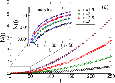
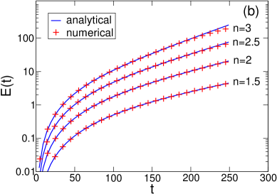
Figure 1: (a) Total number of particles produced in a cavity vibrating with (28) and $\omega=2n\pi$ with $n=1.5,2,2.5$ and $3$. The small plot shows the results in the time range $[0,50]$ together with the analytical prediction (solid line) $N(t)=n(4n^{2}-1)(10^{-3}\pi t)^{2}/12$ of [6, 8] valid for short times $(10^{-3}\pi t)\ll 1$. (b) Numerical results for the created energy $E(t)$ corresponding to (a) together with the analytical prediction $E(t)=(4n^{2}-1)\pi\sinh^{2}(n10^{-3}\pi t)/12$ of [8] (solid line). The results correspond to the largest cut-off parameters as given in Fig. 2.

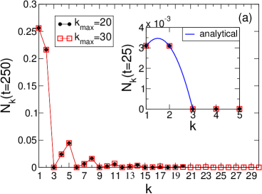
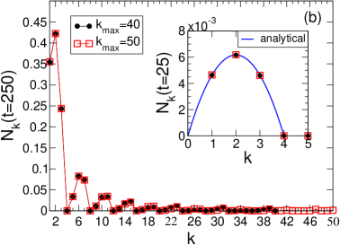
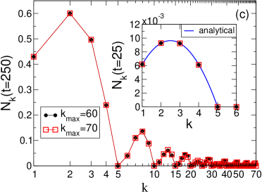
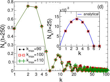
Figure 2: Particle spectra for (a) $\omega=3\pi$, (b) $\omega=4\pi$, (c) $\omega=5\pi$ and (d) $\omega=6\pi$ corresponding to the results shown in Fig. 1. The small plots compare the numerical results for $N_{k}(t=25)$ with the analytical prediction $N_{k}(t)=(2n-k)k(10^{-3}\pi t)^{2}/4$ of [6] plotted for continuous values of $k$ (solid line).

For short times $\epsilon\,\pi\,t=10^{-3}\,\pi\,t\ll 1$ the numerical results are well described by the analytical predictions of [6, 8]. The numerically calculated spectra for times $t=25$ shown in Fig. 2 are well fitted by the analytical expression $N_{k}(t)=(2n-k)k(10^{-3}\pi t)^{2}/4$ for $k<2n$ and $N_{k}(t)=0$ otherwise [6], predicting a parabolic shape of the particle spectrum. More quantitatively, for $n=2$, for instance, the predicted values $N_{1}(t=25)=N_{3}(t=25)\sim 4.63\times 10^{-3}$, $N_{2}(t=25)=6.17\times 10^{-3}$ agree well with the values $N_{1}(t=25)=4.62\times 10^{-3}$, $N_{2}(t=25)=6.14\times 10^{-3}$ and $N_{3}(t=25)=4.59\times 10^{-3}$ obtained from the numerical simulations with $k_{\rm max}=50$. Consequently, the total number of created particles is perfectly described by the expression $N(t)=n(4n^{2}-1)(10^{-3}\pi t)^{2}/12$ [6, 8] as it is demonstrated in the small plot in Fig. 1 (a).

For the entire integration range $[0,250]$ we compare the numerical results for the total energy associated with the created quantum radiation with the analytical expression $E(t)=(4n^{2}-1)\pi\sinh^{2}(n\,10^{-3}\pi t)/12$ [8] predicting that the energy increases exponentially with time [Fig. 1 (b)]. The numerical values and the analytical prediction agree very well for $n=1.5$ and $2$. In the case of $n=2.5$ and $3$ we observe slight deviations towards the end of the integration range. This is due to the numerical instabilities in the corresponding particle spectra [cf Figs. 2 (c) and (d)]. The numerical values for $N_{k}$ with $k$ larger than some value ($k>10$ for $n=3$, for instance) do not remain unchanged when varying $k_{\rm max}$. Even $N_{k}$ is small for the higher frequencies compared to the values of $N_{k}$ for the excited lowest modes their contribution to the total energy is significant because of their high frequency. Hence relatively small instabilities in $N_{k}$ for larger $k$ give rise to a non-stable (with respect to $k_{\rm max})$ result for the energy. In order to gain better agreement of the numerical results for the energy for $n=2.5$ and $3$ with the analytical prediction a further increase of $k_{\rm max}$ is necessary.

We now consider the case of detuning $\omega=2\pi(n+\delta n)$. In an off-resonant vibrating one-dimensional cavity the total energy associated with the created particles may increase exponentially $E(t)=(\pi/12)(4n^{2}-1)\sinh^{2}(n\sqrt{1-\gamma^{2}}\pi 10^{-3}\,t)/(1-\gamma^{2})$ if $\gamma<1$, quadratically $E(t)=(\pi/3)(4n^{2}-1)(n\pi 10^{-3}\,t/2)^{2}$ if $\gamma=1$ or oscillate $E(t)=(\pi/12)(4n^{2}-1)\sin^{2}(n\sqrt{\gamma^{2}-1}\pi 10^{-3}\,t)/(\gamma^{2}-1)$ if $\gamma>1$, depending on the strength of detuning $\delta n$ parametrized by $\gamma=\delta n\times 10^{3}/n$ [8]. In Fig. 3 (a) results for the total energy obtained in simulations with different off-resonant frequencies are shown covering all three different possibilities for $\gamma$ and compared to the analytical predictions. In all cases the numerical results are very well described by the analytical expressions. Figure 3 (b) depicts the periods of the energy (and particle number) oscillations as obtained from the simulations and compares them with the analytical prediction $t_{0}=10^{3}/(n\sqrt{\gamma^{2}-1})$ showing that both are in good agreement. The numerical values for the maximal amplitudes $N(t_{0}/2)$ of the corresponding particle number oscillations are shown in Fig. 3 (c) and fitted to the power law $N(t_{0}/2)\propto(\delta n)^{\alpha}$ with values of $\alpha$ as indicated in the figure.

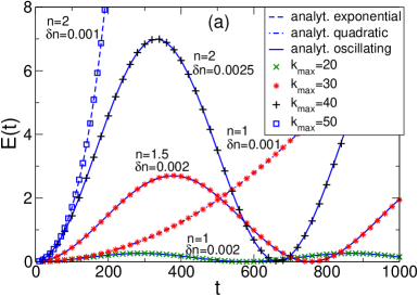
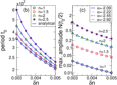
Figure 3: (a) Energy associated with the particles created in an off-resonantly vibrating one-dimensional cavity. Numerical results are compared to the analytical predictions of [8]. The numerical results are always shown for cut-off parameters $k_{\rm max}$ which ensure numerical stability. (b) Period of particle number oscillations caused by detuning. The numerically obtained period is compared with the analytical prediction $t_{0}=10^{3}/(n\sqrt{\gamma^{2}-1})$ of [8]. (c) Maximal amplitude $N(t_{0}/2)$ of the corresponding particle number oscillations fitted to the power law $N(t_{0}/2)\propto(\delta n)^{\alpha}$.

The numerical results presented in this section are entirely in very good agreement with the corresponding analytical predictions derived for small amplitude oscillations $\epsilon\ll 1$ which demonstrates the reliability of the numerical simulations. However, a few critical comments are in order. In our considerations above the analytical expressions have been treated as continuous functions of time. But strictly speaking, they are valid only for times at which the moving wall has returned to its initial position. Moreover, in the numerical simulations the expectation values have been calculated also for times at which the velocity of the moving wall is non-zero (matching problem). Consequently one may expect that part of the particle production is spurious and in particular if modes of arbitrarily high frequency are excited, for instance due to the initial discontinuity in the velocity of the motion (28), and $k_{\rm max}\rightarrow\infty$ the particle number diverges and the numerical results do not agree with the analytical predictions. In the numerical simulations this is automatically avoided due to the cut-off $k_{\rm max}$. Nevertheless, working with a finite cut-off is well motivated because it simulates imperfect boundary conditions for high frequency modes and, as a matter of course, is a necessity for a numerical treatment. For the numerical results presented above these spurious effects are negligibly small and therefore the numerical results agree very well with the analytical predictions. This is due to the fact that we restrict ourselves to small amplitudes $\epsilon\ll 1$ and hence to small velocities. Therefore the effect of the discontinuity in the velocity of the boundary motion on the particle creation is expected to be small. This has been studied for the initial discontinuity in the velocity in [41] in detail demonstrating that the matching problem becomes only important for larger $\epsilon$. In Appendix C we discuss the convergence of the numerical results in comprehension with the numerical accuracy of the simulations for the case $\omega=3\pi$ more detailed.

6 Conclusion

A formalism allowing for numerical investigation of particle creation from vacuum in dynamical cavities, i.e. the dynamical Casimir effect, has been presented. By introducing a particular parametrization for the time-evolution of the field modes inside the dynamical cavity, a system of coupled first-order linear differential equations has been derived. Physical quantities like the number of particles created during the dynamics of the cavity and the associated energy are determined by the solutions to this system which can be found by applying standard numerics.

In continuation of the work [41] we have studied the creation of massless scalar particles due to resonant as well as off-resonant sinusoidal oscillations of one of the cavity walls. The numerical results are entirely in agreement with the analytical predictions derived in [6, 8] demonstrating that the numerical simulations are reliable and the method introduced is appropriate to study the dynamical Casimir effect fully numerically.

Potential problems inherent in the method, in particular the matching problem due to discontinuities in the velocity of the boundary motion yielding spurious contributions to the total particle number, have been discussed. It has been shown that this effect is negligibly small for cavity vibrations with a sufficiently small amplitude.

Being derived very generally, the method is applicable for different kinds of boundary conditions of the form (4) provided that the spectrum $\{\Omega_{n}\}$ contains no zero mode, i.e. $\Omega_{n}>0\;\forall n$ and can easily be extended to massive scalar fields by substituting for the frequency $\Omega_{n}$ the corresponding expression for a massive scalar field, i.e. $\Omega_{n}=\sqrt{(n\pi)^{2}/l^{2}+m^{2}}$ where $m$ is the mass. Furthermore, the generalization to higher dimensional cavities is straightforward. This makes it possible to study the dynamical Casimir effect for a variety of possible interesting scenarios where less or even nothing is known analytically. As already mentioned in the introduction, TE-mode photon creation in a three-dimensional rectangular cavity [23] can be studied with the same method as well because it can be related to the production of massive scalar particles in a one-dimensional cavity [42]. However, more complicated boundary conditions than (4) appearing for example when studying TM-mode photons [27] cannot be treated within this approach.

Appendix A Derivation of $\xi_{n}^{(m)}$ and $\eta_{n}^{(m)}$

The auxiliary functions $\xi_{n}^{(m)}(t)$ and $\eta_{n}^{(m)}(t)$ [Eqs. (19), (20)] can be introduced in the following way: Define an operator $\hat{b}_{n}(t)$ via $\hat{b}_{n}(t):=\hat{U}^{\dagger}(t,0)\,\hat{a}_{n}\,\hat{U}(t,0)$ with $\hat{a}_{n}$ being the annihilation operator corresponding to the initial state [Eq. (6)], i.e. $\hat{a}_{n}=(1/\sqrt{2})[\sqrt{\Omega_{n}^{0}}\hat{q}_{n}(0)+(i/\sqrt{\Omega_{n}^{0}})\hat{p}_{n}(0)]$. Hence $\hat{b}_{n}(t)=(1/\sqrt{2})[\sqrt{\Omega_{n}^{0}}\hat{U}^{\dagger}(t,0)\hat{q}_{n}(0)\hat{U}(t,0)+(i/\sqrt{\Omega_{n}^{0}})\hat{U}^{\dagger}(t,0)\hat{p}_{n}(0)\hat{U}(t,0)]$. By using Eqs. (13) and (14) one derives

$$\hat{b}_{n}(t\geq 0)=\sum_{m}\frac{1}{2}\sqrt{\frac{\Omega_{n}^{0}}{\Omega_{m}^{0}}}\left[\xi_{n}^{(m)}(t)\;\hat{a}_{m}+\eta_{n}^{(m)^{*}}(t)\;\hat{a}_{m}^{\dagger}\right]$$ (30)

with $\xi_{n}^{(m)}(t)$ and $\eta_{n}^{(m)}(t)$ defined in Eqs. (19) and (20). Note that this definition of the time evolution for $\hat{b}_{n}(t)$ does not account for an explicit time-dependence of $\hat{b}_{n}(t)$. Therefore, in general, no meaningful notion of particles may be assigned to the operator $\hat{b}_{n}(t)$. This manifests itself in the relation between the operator $\hat{A}_{n}$ corresponding to the particle notion for $t\geq t_{1}$ [Eq. (7)] and the operators $\hat{b}_{n}(t_{1})$, $\hat{b}^{\dagger}_{n}(t_{1})$ given by

$$\hat{A}_{n}=\sqrt{\frac{\Omega_{n}^{1}}{\Omega_{n}^{0}}}\left[\Delta_{n}^{+}(t_{1})\,\hat{b}_{n}(t_{1})+\Delta_{n}^{-}(t_{1})\,\hat{b}_{n}^{\dagger}(t_{1})\right]$$ (31)

with $\Delta_{n}^{\pm}(t)$ defined in (23). Equation (31) follows directly from Eq.(9) with (21), (22) and (30). For motions ending at $t=t_{1}$ with $l(t_{1})\neq l_{0}$ the operator $\hat{b}_{n}(t)$ has not evolved into the operator $\hat{A}_{n}$ associated with the correct particle notion after the dynamics. However, if $l(t_{1})=l_{0}$, for example when $t_{1}$ is a multiple of the period of boundary vibrations, $\hat{A}_{n}=\hat{b}_{n}(t_{1})$.

Appendix B The system for ${\cal A}_{n}^{(m)}$ and ${\cal B}_{n}^{(m)}$

Taking the stopping time $t_{1}$ in (16) and (17) to be a continuous variable one derives the following system of coupled differential equations for ${\cal A}_{mn}$ and ${\cal B}_{mn}$:

$$\dot{\cal A}_{mn}=-i\Omega_{n}{\cal A}_{mn}+\Gamma_{n}{\cal B}_{mn}+\sum_{k}\left[K_{nk}^{-}{\cal A}_{mk}-K_{nk}^{+}{\cal B}_{mk}\right]$$ (32)

$$\dot{\cal B}_{mn}=-i\Omega_{n}{\cal B}_{mn}+\Gamma_{n}{\cal A}_{mn}+\sum_{k}\left[K_{nk}^{-}{\cal B}_{mk}-K_{nk}^{+}{\cal A}_{mk}\right]$$ (33)

with

$$\Gamma_{n}(t)=\frac{1}{2}\frac{\dot{\Omega}_{n}(t)}{\Omega_{n}(t)}\;,\;\;K_{nk}^{\pm}(t)=\frac{1}{2}\left[\sqrt{\frac{\Omega_{k}(t)}{\Omega_{n}(t)}}M_{nk}(t)\pm\sqrt{\frac{\Omega_{n}(t)}{\Omega_{k}(t)}}M_{kn}(t)\right].$$ (34)

Appendix C Numerics

The numerical simulations have been performed by using a Runge-Kutta Prince-Dormand method (rk8pd) based on source code provided by the GNU Scientific Library (GSL) [44]. In the table in Fig. 4 we show the numerical values for the total number of particles $N(t)$ created in a cavity subject to sinusoidal oscillations of the form (28) with frequency $\omega=3\pi$ [cf. Figs. 1 and 2 (a)] for two times $t=249.5$ and $t=250.0$ and cut-off parameters $k_{\rm max}=20,30,40,50$ and $60$. The plot in Fig. 4 shows the diagonal part of the first of the Bogoliubov relations (10) $d_{k}=1-\sum_{m}(|{\cal A}_{mk}|^{2}-|{\cal B}_{mk}|^{2})=0$ for $k=1,...,10$ and $51,...,60$ computed from the solutions of the simulation with $k_{\rm max}=60$. The absolute and relative errors for the rk8pd routine in the simulations have been set to $10^{-8}$.

$k_{\rm max}$	$N(t=249.5)$	$N(t=250.0)$
20	0.5799007	0.5823052
30	0.5798943	0.5822980
40	0.5798951	0.5822983
50	0.5798956	0.5822984
60	0.5798959	0.5822984

Figure 4: Left: Plot showing the numerically evaluated diagonal part of the first of the Bogoliubov relations (10) $d_{k}=1-\sum_{m}(|{\cal A}_{mk}|^{2}-|{\cal B}_{mk}|^{2})$ for the lowest frequencies $k=1,...,10$ as well as $k=51,...,60$ corresponding to the simulation with cut-off $k_{\rm max}=60$. Right: Table showing the numerical values of the total particle number at times $t=249.5$ and $t=250$ obtained for $\omega=3\pi$ and $k_{\rm max}=20,30,40,50$ and $60$.

The plot demonstrates that for those settings $d_{k}=0$ is satisfied by the numerical solutions up to $\sim 3\times 10^{-5}$ at the end of the integration range. Thereby the accuracy is better for the lowest modes $k=1,...,10$ than for the modes $k=51,...,60$. This is partly due to the fact that the higher modes are more affected by the truncation of the infinite system at $k_{\rm max}=60$ than the lowest modes. The accuracy for the intermediate modes $k=11,...,50$ lies in between the two “bands” visible in the plot. The remaining Bogoliubov relations are satisfied with at least the same accuracy demonstrating that the numerical errors are small compared to the values of the particle numbers itself. We consider $d_{k}$ as the determining measure for the accuracy of the numerical calculations which can be easily enhanced further by increasing the preset accuracy of the integration routine.

The numerical values for $N(t=249.5)$ and $N(t=250.0)$ summarized in the table in Fig. 4 are shown with seven decimal places. Varying the cut-off between $k_{\rm max}=30$ and $60$ both values change only in the last two of the shown seven decimal places and therefore the variation in $N(t)$ when changing $k_{\rm max}$ is smaller than $10^{-5}$, i.e. smaller than the numerical error in the Bogoliubov relations. This demonstrates that the convergence of the numerical values for $N(t)$ is sufficiently good. Furthermore, because $\dot{l}(t=250)=3\pi\epsilon$ ($l_{0}=1$) we can conclude that spurious effects caused by discontinuities in the velocity (matching problem) are indeed negligibly small for the parameters considered ($\epsilon\ll 1$).

References

- [1] V. V. Dodonov, in Nonstationary Casimir effect and analytical solutions for quantum fields in cavities with moving boundaries, in M. W. Evans (Ed), Modern Nonlinear Optics, Advances in Chemical Physics Series, Wiley, New York, Vol 119, Part 1, 309 (2001).
- [2] A. Lambrecht, M.-T. Jaekel, and S. Reynaud, Phys. Rev. Lett. 77, 615 (1996).
- [3] V. V. Dodonov and A. B. Klimov, and D. E. Nikonov, J. Math. Phys. 34, 2742 (1993).
- [4] V. V. Dodonov and A. B. Klimov, Phys. Rev. A. 53, 2664 (1996).
- [5] V. V. Dodonov, Phys. Lett. A 213, 219 (1996).
- [6] J.-Y. Ji, H.-H. Jung, J.-W. Park, and K.-S. Soh, Phys. Rev. A. 56, 4440 (1997).
- [7] R. Schützhold,G. Plunien and G. Soff, Phys. Rev. A 57, 2311 (1998).
- [8] V. V. Dodonov, J. Phys. A: Math. Gen. 31, 9835 (1998).
- [9] A. B. Klimov and V. Altuzar, Phys. Lett. A 226, 41 (1997).
- [10] L.-P. Fu, C. K. Duan, and G.-C. Guo, Phys. Lett. A 234, 163 (1997).
- [11] A. V. Chizhov, G. Schrade and M. S. Zubairy, Phys. Lett. A 230, 269 (1997).
- [12] C. K. Law, Phys. Rev. Lett. 73, 1931 (1994).
- [13] C. K. Cole and W. C. Schieve, Phys. Rev. A. 52, 4405 (1995).
- [14] O. Méplan and C. Gignoux, Phys. Rev. Lett. 76, 408 (1996).
- [15] D. A. R. Dalvit and F. D. Mazzitelli, Phys. Rev. A. 57, 2113 (1998).
- [16] P. Wegrzyn, T. Rog, Act. Phys. Pol. B32, 129 (2001).
- [17] M. A. Andreata and V. V. Dodonov, J. Phys. A 33, 3209 (2000).
- [18] R. de la Llave and N. P. Petrov, Phys. Rev. E 59, 6637 (1999).
- [19] L. H. Ford and A. Vilenkin, Phys. Rev. D 25, 2569 (1982).
- [20] G. Barton and C. Eberlein, Ann. Phys. (N.Y.) 227, 222 (1993).
- [21] P. A. Maia Neto, J. Phys. A 27, 2167 (1994).
- [22] D. F. Mundarain and P. A. Maia Neto, Phys. Rev. A 57, 1379 (1998).
- [23] M. Crocce, D. A. R. Dalvit, and F. D. Mazzitelli, Phys. Rev. A. 64, 013808 (2001).
- [24] V. V. Dodonov, Phys. Lett. A 207, 126 (1995).
- [25] A. V. Dodonov, E. V. Dodonov, and V. V. Dodonov, Phys. Lett. A 317, 378 (2003).
- [26] A. V. Dodonov and V. V. Dodonov, Phys. Lett. A 289, 291 (2001).
- [27] M. Crocce, D. A. R. Dalvit and F. D. Mazzitelli, Phys. Rev. A. 66, 033811 (2002).
- [28] V. V. Dodonov, Phy. Lett. A 244, 517 (1998).
- [29] V. V. Dodonov, Phy. Rev. A 58, 4147 (1998).
- [30] G. Schaller, R. Schützhold, G. Plunien and G. Soff, Phys. Lett. A 297, 81 (2002).
- [31] G. Schaller, R. Schützhold, G. Plunien and G. Soff, Phy. Rev. A 66, 023812 (2002).
- [32] G. Plunien, R. Schützhold, and G. Soff, Phys. Rev. Lett. 84, 1882 (2000).
- [33] R. Schützhold, G. Plunien, and G. Soff, Phys. Rev. A 65, 043820 (2002).
- [34] H. Jing, Q.-Y. Shi, and J.-S. Wu, Phys. Lett. A 268, 174 (2000).
- [35] C. K. Law, Phys. Rev. A 51, 2537 (1995).
- [36] R. Golestanian and M. Kardar, Phys. Rev. Lett. 78, 3421 (1997).
- [37] C. K. Cole and W. C. Schieve, Phys. Rev. A. 64, 023813 (2001).
- [38] N. D. Antunes, hep-ph/0310131 v1 (2003).
- [39] L. Li and B. Z. Li, Phys. Lett. A, 300, 27 (2002).
- [40] A. Fedotov, N. Narozhny, and Y. Lozovik, J. Opt. B: Quantum Semiclass. Opt. 7, S64 (2005).
- [41] M. Ruser, J. Opt. B: Quantum Semiclass. Opt. 7, S100 (2005).
- [42] M. Ruser, quant-ph/0509030 (2005).
- [43] C. Cartier, R. Durrer, and M. Ruser, Phys. Rev. D 72, 104018 (2005).
- [44] http://www.gnu.org/software/gsl/