Scheme for generating a sequence of single photons of alternating polarisation

Abstract

Single-photons of well-defined polarisation that are deterministically generated in a single spatio-temporal field mode are the key to the creation of multi-partite entangled states in photonic networks. Here, we present a novel scheme to produce such photons from a single atom in an optical cavity, by means of vacuum-stimulated Raman transitions between the Zeeman substates of a single hyperfine state. Upon each transition, a photon is emitted into the cavity, with a polarisation that depends on the direction of the Raman process.

I Introduction

Worldwide, large efforts are being made to interface single atoms with single photons, since this is the key to the entanglement Cabrillo99 ; Browne03 ; Duan03 ; Blinov04 and teleportation Bose99 ; Lloyd01 of quantum states between distant atoms. Transform-limited and mutually coherent single photons in well-defined polarisation and spatio-temporal field modes are needed so that the desired quantum-correlation effects occur Knill01 ; Hong87 ; Legero03 . Some crucial problems that arise in the production of such photons have been solved, such as the choice of an adequate emitter, the efficient collection of the emitted photons or their channelling into a given direction. In particular, several research groups have demonstrated that strongly coupled atom-cavity systems can be used as deterministic sources of single photons Kuhn02 ; Keller04 ; McKeever04 . In these experiments, a single atom located in the cavity is exposed to laser pulses which drive one branch of a Raman transition. The other branch is resonant with the cavity mode so that the field mode of the cavity receives one photon upon each successful Raman transition. The photons are finally emitted from the cavity, and Hanbury Brown & Twiss photon-correlation measurements are used to demonstrate the single-photon nature of the emission.

In this article, we propose to extend this photon-generation scheme in such a way that single photons of well-defined polarisation are emitted from a coupled atom-cavity system. This new method is based on our previous work Hennrich00 ; Kuhn02 ; Hennrich03 ; Legero04 , where Raman transitions between hyperfine states of a ⁸⁵Rb atom were used to generate single photons. The large number of accessible magnetic sublevels in ⁸⁵Rb meant that the polarisation of these photons was undefined. In order to achieve polarisation control, we now investigate the situation shown in Fig. 1. Vacuum-stimulated Raman transitions are considered between the $m_{F}=\pm 1$ Zeeman substates of an $F=1$ hyperfine state, e.g. in the electronic ground state of ⁸⁷Rb atoms. We assume a magnetic field along the cavity axis that lifts the degeneracy of the magnetic substates. If the frequency of the applied laser pulses is either red or blue detuned from the unperturbed transition by twice the B-field induced Zeeman shift, while the cavity frequency is in resonance with the unperturbed atomic transition, then the transition between the $m_{F}=+1$ and $m_{F}=-1$ levels is resonantly driven by laser and cavity, but with their roles changing as a function of the chosen laser detuning. In this way the Raman transition can be driven in one or the other direction, leading to an emission of either $\sigma^{+}$ or $\sigma^{-}$ photons. As can be seen in the level scheme shown in Fig. 1, this method requires the laser to be polarised perpendicular to the cavity axis, so that it decomposes into $\sigma^{+}$ and $\sigma^{-}$ polarisation components with respect to the magnetic field direction. Only the $\sigma^{+}$ polarisation component of the driving laser is used for the generation of a $\sigma^{-}$ polarised photon and vice versa. The other polarisation component of the laser pulse is always present, but it is out-of-resonance with all relevant atomic transitions.

As the cavity supports both polarisation modes, alternating the laser frequency between the two possible resonances from pulse to pulse should be sufficient to generate a sequence of single photons of alternating polarisation. No repumping of the atom to its initial state is required from one photon to the next, since the final state reached with a $\sigma^{+}$ photon emission is at the same time the initial state for producing a $\sigma^{-}$ photon with the subsequent driving laser pulse, and vice versa. With this novel scheme, one should therefore be able to produce sequences of photons with well-defined polarisation.

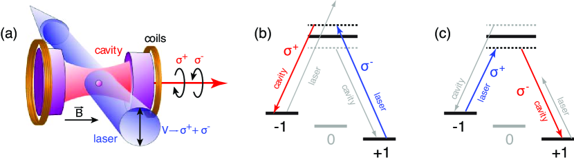
Figure 1: Principle of the photon generation scheme. A single atom is strongly coupled to an optical cavity, and a magnetic field acting along the cavity axis lifts the degeneracy of the Zeeman substates (a). From the side, laser pulses drive Raman transitions in the atom. The polarisation of the laser is perpendicular to the cavity and B-field axis, so that it decomposes into $\sigma^{+}$ and $\sigma^{-}$ components with respect to the cavity. As illustrated in (b) and (c), the cavity is resonant with the non-shifted atomic transition, but the laser pulse is red or blue detuned: a blue detuned laser pulse drives a Raman transition from $m_{F}=+1$ to $m_{F}=-1$ and generates a $\sigma^{+}$ polarised photon (b), while a red detuned laser pulse drives the transition in the opposite direction and generates a $\sigma^{-}$ polarised photon (c).

II The ideal three-level atom

For an illustration of the photon generation process, we first consider an idealised atom with an $F=1$ hyperfine ground state and an $F^{\prime}=0$ electronically excited state. The Zeeman shift induced by the magnetic field on the $m_{F}=\pm 1$ atomic ground states is $\mp\Delta_{B}=\mp|g_{L}|\mu_{B}B$, where $\mu_{B}$ is the Bohr magneton and $g_{L}$ the Landé factor. In the following the $m_{F}=\{-1,0,+1\}$ Zeeman substates of the $F=1$ ground state will be written as $|{\scriptstyle-}\rangle$,$|0\rangle$ and $|{\scriptstyle+}\rangle$, whereas the $F^{\prime}=0$ excited state is labelled $|e\rangle$. For geometric reasons the cavity supports only $\sigma^{+}$ and $\sigma^{-}$ photons, which have identical frequencies if the relevant cavity modes are degenerate. The state of the coupled atom-cavity system can therefore be written as a superposition of product states $|i,n_{+},n_{-}\rangle$, with $i$ representing the atomic state, and $n_{\pm}$ denoting the number of $\sigma^{\pm}$ photons. In this paper we restrict the number of photons in each mode to zero or one, since higher photon numbers are very unlikely. Note that the cavity couples only product states of different photon numbers, while the interaction of the atom with the pump laser leaves the intra-cavity photon number unchanged. The pump frequency $\omega_{p}$ and the cavity resonance frequency $\omega_{c}$ are both close to the $|0\rangle$ to $|e\rangle$ transition frequency $\omega_{0e}$. We also disregard the states $|0,n_{+},n_{-}\rangle$, since $|0\rangle$ is decoupled from all other internal states. In this way an atomic three-level system in a $\Lambda$-configuration is obtained. Here, we choose the energy of the excited state $|e,0,0\rangle$ to define the origin of the energy scale and we divide the Hamiltonian of the system into two parts, $\hat{H}=\hat{H}_{stat}+\hat{H}_{int}$. The stationary part $\hat{H}_{stat}$ includes the energy levels of atom and cavity, and $\hat{H}_{int}$ describes the interaction of the atom with pump laser and cavity. The system is examined in the interaction picture. In the rotating wave approximation, the stationary part of the Hamiltonian reads

$$\hat{H}_{stat}=\hat{H}_{atom}+\hat{H}_{cavity}=\hbar\Big{[}\left(\Delta_{p}+\Delta_{B}\right)|{\scriptstyle-}\rangle\langle{\scriptstyle-}|+\left(\Delta_{p}-\Delta_{B}\right)|{\scriptstyle+}\rangle\langle{\scriptstyle+}|\Big{]}+\hbar\Delta_{cp}\left(\hat{a}^{{\dagger}}\hat{a}+\hat{b}^{{\dagger}}\hat{b}\right),$$ (1)

where $\Delta_{p}\equiv\omega_{p}-\omega_{0e}$ is the detuning of the pump laser from the transition between $|0\rangle$ and $|e\rangle$ and $\Delta_{cp}\equiv\omega_{c}-\omega_{p}$ is the difference between cavity resonance and pump laser frequency. Here, $\hat{a}^{{\dagger}}$ and $\hat{a}$, or $\hat{b}^{{\dagger}}$ and $\hat{b}$, are the creation and annihilation operators of a photon in the $\sigma^{+}$ or $\sigma^{-}$ polarised cavity mode, respectively. The interaction between atom and cavity is given by the interaction Hamiltonian

$$H_{int}=-\hbar\left[g\left(|e\rangle\langle{\scriptstyle-}|\hat{a}+\hat{a}^{{\dagger}}|{\scriptstyle-}\rangle\langle e|+|e\rangle\langle{\scriptstyle+}|\hat{b}+\hat{b}^{{\dagger}}|{\scriptstyle+}\rangle\langle e|\right)+\frac{1}{2}\Omega\Big{(}|e\rangle\langle{\scriptstyle-}|+|{\scriptstyle-}\rangle\langle e|+|e\rangle\langle{\scriptstyle+}|+|{\scriptstyle+}\rangle\langle e|\Big{)}\right],$$ (2)

where g is the coupling constant of the atom to both cavity modes (assumed to be equal), and $\Omega$ is the Rabi frequency of the pump laser.

The cavity decay gives rise to the emission of photons from the cavity, which is a non-unitary process. It cannot be included in a Hermitian Hamiltonian, but its effects on the density matrix can be expressed by the Liouville operator Scully97 ,

$$\hat{L}[\hat{\rho}]=\kappa\left(2\hat{a}\hat{\rho}\hat{a}^{{\dagger}}-\hat{a}^{{\dagger}}\hat{a}\hat{\rho}-\hat{\rho}\hat{a}^{{\dagger}}\hat{a}+2\hat{b}\hat{\rho}\hat{b}^{{\dagger}}-\hat{b}^{{\dagger}}\hat{b}\hat{\rho}-\hat{\rho}\hat{b}^{{\dagger}}\hat{b}\right).$$ (3)

The cavity field decay rate $\kappa$, here identical for both polarisations, has to be fast with respect to the Raman process to ensure that the photon is emitted from the cavity before being reabsorbed by the atom.

The time evolution of the system is then given by the master equation

$$\frac{d}{dt}\hat{\rho}=-\frac{i}{\hbar}[\hat{H},\hat{\rho}]+\hat{L}[\hat{\rho}].$$ (4)

Note that a similar Raman process driven in only one direction has been discussed previously in Kuhn99 . Here, we search for conditions where Raman transitions can be driven in both directions, albeit with the cavity frequency fixed. This imposes new constraints, and we now have to determine the optimal parameters for efficient production of $\sigma^{+}$ and $\sigma^{-}$ photons.

The initial state of the system is set to $|\Psi_{start}\rangle=|{\scriptstyle+},0,0\rangle$ and realistic cavity parameters are chosen, $(g;\kappa;\Delta_{B})/2\pi=(2.7;1.25;15)$ MHz (e.g. corresponding to a ⁸⁷Rb atom in the 5S${}_{1/2}|F=1,m_{F}=+1\rangle$ hyperfine ground state and excitation of the D₂-line, inside a cavity used in former experiments Kuhn02 ; Hennrich00 ; Hennrich03 ; Legero04 and a magnetic field of 21.4 G). The cavity is in resonance with the $|0\rangle$ to $|e\rangle$ transition, (i.e. $\omega_{c}=\omega_{0e}$), and in order to resonantly drive the Raman transition from $|{\scriptstyle+},0,0\rangle$ to $|{\scriptstyle-},1,0\rangle$, the pump laser has to have a detuning of $\Delta_{p}=+2\Delta_{B}$. The pump-laser Rabi frequency follows a $\sin^{2}(\pi t/1.5\mu s)$-pulse amplitude with a peak value of $\Omega/2\pi=6$ MHz for each polarisation, as shown in Fig. 2 (a).

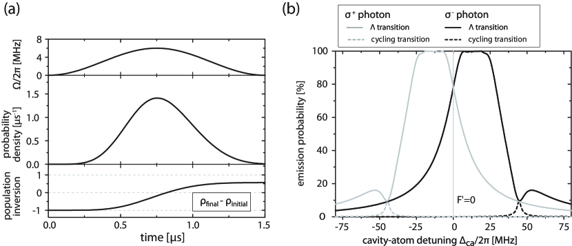
Figure 2: Results for the idealised three-level atom with parameters $(g;\kappa;\Delta_{B})/2\pi$ = (2.7; 1.25; 15) MHz. (a) Time evolution of the system: pump laser Rabi-frequency $\Omega/2\pi$ follows a $\sin^{2}(\pi t/1.5\mu s)$-pulse amplitude, with a peak value of 6 MHz. The probability density for generating a photon per $\mu s$ is shown. Integrating over the whole pulse gives an emission probability of $78\%$ per pulse. Accordingly, the population transfer between the atomic state, defined by the difference in population of the final and initial state, ends up at an inversion of 0.56. (b) Photon production efficiency as a function of the cavity-atom detuning $\Delta_{ca}$. The pump laser is always tuned to the desired Raman resonance: for $\sigma^{-}$ photons $\Delta_{cp}=-2\Delta_{B}$, for $\sigma^{+}$ photons $\Delta_{cp}=+\Delta_{B}$. Black lines stand for the probability for generating $\sigma^{-}$ photons, grey lines for $\sigma^{+}$ photons, whereas solid lines indicate the desired $\Lambda$-type transition, and dashed lines the cycling transitions, starting and ending in the same state.

The probability density for emitting a photon varies as a function of time, and reflects the envelope of the generated single-photon wave packet. Note that the shape of the photon depends on the driving field. Changing the shape of the pump pulse or its peak value has a direct impact on the emission probability. The photon can therefore be shaped in many desired ways. The integral of the probability density over the whole photon duration gives the overall emission probability of a photon, here it measures $78\%$. The lower part of Fig. 2 (a) illustrates the population inversion between the states $|{\scriptstyle-}\rangle$ and $|{\scriptstyle+}\rangle$, which is here the population difference between the final and the initial atomic state. The inversion starts from $-1$ at $t=0$ and increases until it reaches $+0.56$. Note that any losses out of the system (except for cavity decay) have been omitted in this simplified model, therefore population which is not transferred into the other ground state simply stays in the initial state. Under these conditions, the emission probability equals the fraction of transferred population. This is not the case in general, since other loss channels than the cavity might exist.

During the population transfer from the state $|{\scriptstyle+},0,0\rangle$ to $|{\scriptstyle-},1,0\rangle$, the single photon state of the cavity decays. Since the time constant 2$\kappa$ is much faster than the duration of the pump pulse, the photon leaks out of the cavity during its generation. Once the atom has reached the state $|{\scriptstyle-},0,0\rangle$, it will be very unlikely to undergo another Raman transition back to the initial state, since the back transition is detuned by $4\Delta_{B}$ (see Fig. 1 (b), grey lines) which is much larger than the cavity linewidth of 2$\kappa$. This means a second emission is suppressed and thus only a single $\sigma^{+}$ or $\sigma^{-}$ photon is generated. The efficiency of the photon generation depends on many parameters. Here it is $78\%$, but it can rise up to $100\%$ with increasing pump power or with a stronger atom-cavity coupling. For a larger Zeeman splitting the emission probability would decrease.

Exactly the same photon generation efficiency and photon envelope are obtained when the initial state is $|{\scriptstyle-},0,0\rangle$ and the detuning of the pump laser frequency is $\Delta_{p}=-2\Delta_{B}$. Then Raman resonance is fulfilled for the $\Lambda$-type transition shown in Fig. 1 (c) and a $\sigma^{-}$ photon is generated. Both cases are similar, since the cavity frequency has been chosen to be on the unshifted transition from $F=1$ to $F^{\prime}=0$, leading to an atom-cavity detuning of $\pm\Delta_{B}$ with respect to the atomic resonances from $|{\scriptstyle+}\rangle$ to $|e\rangle$ and $|{\scriptstyle-}\rangle$ to $|e\rangle$. This symmetry is only broken when we detune the cavity. In Fig. 2 (b), the photon generation efficiencies are plotted as a function of the cavity-atom detuning, $\Delta_{ca}\equiv\omega_{c}-\omega_{0e}$, with the pump frequency always chosen in such a way that laser and cavity are in Raman resonance with either the $|{\scriptstyle+}\rangle$ to $|{\scriptstyle-}\rangle$ or the $|{\scriptstyle-}\rangle$ to $|{\scriptstyle+}\rangle$ transition, i.e. $\Delta_{cp}=\pm 2\Delta_{B}$. Black lines indicate the probability to emit a $\sigma^{-}$ photon and grey lines a $\sigma^{+}$ photon. The solid lines give the efficiencies for the photon production within the desired $\Lambda$-type Raman transitions, i.e. starting in $|{\scriptstyle+}\rangle$ and ending in $|{\scriptstyle-}\rangle$ for $\sigma^{+}$ or vice versa for $\sigma^{-}$ photons. Driving a $\Lambda$-type transition with a cavity-atom detuning around $\Delta_{ca}=-\Delta_{B}$ for $\sigma^{+}$ photons (grey line) or $\Delta_{ca}=+\Delta_{B}$ for $\sigma^{-}$ photons (black line) leads to 100$\%$ efficiency of the process. In both cases, the detuning of the cavity compensates the Zeeman shift and both arms of the Raman resonance coincide with an atomic resonance. However, to generate $\sigma^{+}$ and $\sigma^{-}$ polarised photons with the same probability in case of a fixed cavity detuning, we have to accept a compromise, i.e. $\Delta_{ca}=0$ with an emission probability reduced to $78\%$.

To verify whether no unwanted second photon will emerge from the system, we also have calculated the probability for a photon production from an atom starting in the wrong initial state, e.g. state $|{\scriptstyle-}\rangle$ for $\sigma^{+}$ photons. If $\sigma^{+}$ photons can be generated in this case, the atom would undergo a cycling transition, since initial and final state are the same. As indicated by the grey dashed line (black dashed line for the analogous case with $\sigma^{-}$ photons) in Fig. 2 (b) the probability for such cycling transitions is close to zero in the frequency range around $\Delta_{ca}=0$, where the scheme for generating photons of alternating polarisation works best, so no second photon will be emitted. Only when the pump laser accidently hits an atomic resonance does the emission probability become non-negligible. This phenomenon is however an artefact of our simplified model, the peaks appearing because the spontaneous decay of the excited atomic state has been omitted. Consequently, once the atom is in the excited state it can only emit into the far-off resonant cavity mode. In a real atom the spontaneous decay to other states would dominate the atom’s behaviour. This is discussed in more detail below.

This simple model shows that, for $\Delta_{ca}=0$, single-photon polarisation control can be achieved by choosing the appropriate pump-laser frequencies. There is no need to alter the cavity frequency or the pump polarisation. Moreover, the probability to emit two photons during the same pump pulse is vanishingly small.

III Polarised photons from alkali atoms

To analyse the behaviour of a coupled atom-cavity system under more realistic conditions, all relevant atomic levels and the spontaneous decay of the excited states must be taken into account. As an example we consider the D₂-line of ⁸⁷Rb. Its 5S_1/2 ground state decomposes into two hyperfine states, $F=\{1;2\}$, with $2\pi\times$6.8 GHz hyperfine splitting, while the 5P_1/2 excited state has four hyperfine substates, $F^{\prime}=\{0;1;2;3\}$, with splittings of $2\pi\times$(72; 157; 267) MHz. The two 5S_1/2($F=1$,$m_{F}=\pm 1$) states are the $|\pm\rangle$ states in our scheme, while the virtual excited level of the Raman transition is some superposition of 5P_1/2($m_{F^{\prime}}$=0) states. Note that the origin of our energy scale is chosen to coincide with $F^{\prime}=0$. This state is still labelled $|e\rangle$. In the ground state, $F=2$ is so far from resonance with pump and cavity that there is effectively no coupling. Therefore spontaneous emissions into $F=2$ constitute an additional loss channel, but the state as such need not be considered. Moreover, we restrict ourselves to a situation where the cavity frequency is near resonant with the transitions from $F=1$ to $F^{\prime}=\{0;1\}$. With a distance of $2\pi\times$157 MHz between $F^{\prime}=1$ and $F^{\prime}=2$, the latter state is far from resonance. Combined with the fact that the dipole-matrix elements for transitions between $F=1$ and $F^{\prime}=2$ are smaller than those for the relevant transitions to $F^{\prime}=\{0;1\}$ the $F^{\prime}=2$ state can be neglected. We also omit the $F^{\prime}=3$ state, since it does not couple to $F=1$.

$\mathcal{A}_{ij}$	$|F^{\prime}=0,m_{F^{\prime}}=0\rangle$	$|F^{\prime}=1,m_{F^{\prime}}=+1\rangle$	$|F^{\prime}=1,m_{F^{\prime}}=0\rangle$	$|F^{\prime}=1,m_{F^{\prime}}=-1\rangle$
$|F=1,m_{F}=+1\rangle$	$\sqrt{\frac{1}{6}}$	$\sqrt{\frac{5}{24}}$	$-\sqrt{\frac{5}{24}}$	-
$|F=1,m_{F}=0\rangle$	$\sqrt{\frac{1}{6}}$	$\sqrt{\frac{5}{24}}$	-	$-\sqrt{\frac{5}{24}}$
$|F=1,m_{F}=-1\rangle$	$\sqrt{\frac{1}{6}}$	-	$\sqrt{\frac{5}{24}}$	$-\sqrt{\frac{5}{24}}$

Table 1: The angular part of the dipole matrix elements $\mathcal{A}_{ij}$ for the transition between $|i\rangle$ and $|j\rangle$. With these numbers, the Rabi frequencies are $\Omega_{ij}=\mathcal{A}_{ij}\cdot\Omega_{0}$. For a transition where $\Delta m=+1$ the cavity coupling constant reads $g^{+}_{ij}=\mathcal{A}_{ij}\cdot g_{0}$, for transitions with $\Delta m=-1$ it is $g^{-}_{ij}=\mathcal{A}_{ij}\cdot g_{0}$ and $g^{\pm}_{ij}=0$ in all other cases. The indices $i$ and $j$ refer to the states $|F,m_{F}\rangle$ and $|F^{\prime},m_{F^{\prime}}\rangle$. The electronic parts of the coupling constant and Rabi frequency are chosen to be $g_{0}/2\pi=6.7$ MHz and $\Omega_{0}/2\pi=14.7$ MHz. Note that in our scheme only $\sigma^{\pm}$ transitions are accessible. The $\mathcal{A}_{ij}$ for the non-relevant $\pi$ transitions are shown in grey.

The stationary part of the Hamiltonian now includes all involved atomic levels. It reads

$$\hat{H}_{stat}=\hbar\left(\sum_{i}\Delta_{i}|i\rangle\langle i|+\Delta_{cp}\left(\hat{a}^{{\dagger}}\hat{a}+\hat{b}^{{\dagger}}\hat{b}\right)\right).$$ (5)

Here, $\Delta_{i}$ stands for the energy of the respective atomic level in the rotating frame, including pump detuning and Zeeman shift with respect to the zero level of our calculation. The interaction part of the Hamiltonian can be written as

$$\hat{H}_{int}=-\hbar\sum_{i,j}\left[g^{+}_{ij}\left(|i\rangle\langle j|\hat{a}^{{\dagger}}+|j\rangle\langle i|\hat{a}\right)+g^{-}_{ij}\left(|i\rangle\langle j|\hat{b}^{{\dagger}}+|j\rangle\langle i|\hat{b}\right)+\frac{1}{2}\Omega_{ij}\Big{(}|i\rangle\langle j|+|j\rangle\langle i|\Big{)}\right],$$ (6)

where $i$ and $j$ denote ground and excited states, respectively. Transitions between $|i\rangle$ and $|j\rangle$ are either driven by the pump with a Rabi frequency $\Omega_{ij}$, or by the coupling of the atom to the $\sigma^{\pm}$ cavity modes, with the atom-cavity coupling constants $g^{\pm}_{ij}$. Both $\Omega_{ij}$ and $g^{\pm}_{ij}$ depend on the angular part $\mathcal{A}_{ij}$ of the dipole matrix elements listed in Tab. 1 Metcalf99 ; Steck01 . We have to distinguish between $\sigma^{+}$ and $\sigma^{-}$ cavity coupling constants. They read $g^{\pm}_{ij}=\mathcal{A}_{ij}\cdot g_{0}$, but $g^{+}_{ij}$ is zero unless $\Delta m\equiv m_{F^{\prime}}-m_{F}=+1$ and $g^{-}_{ij}$ is zero unless $\Delta m=-1$. For the relevant transitions, also the Rabi frequencies read $\Omega_{ij}=\mathcal{A}_{ij}\cdot\Omega_{0}$. For our calculation, we have chosen realistic values for the electronic parts of the atom-cavity coupling and of the peak Rabi frequency, i.e. $g_{0}/2\pi=6.7$ MHz and $\Omega_{0}/2\pi=14.7$ MHz.

To include the spontaneous decay of the involved excited states, we extend the Liouville operator (3) to

$$\hat{L}[\hat{\rho}]=\sum_{i,j}\left[\gamma_{ij}\Big{(}2|i\rangle\langle j|\hat{\rho}|j\rangle\langle i|\Big{)}\right]-\sum_{j}\gamma_{j}\Big{(}|j\rangle\langle j|\hat{\rho}+\hat{\rho}|j\rangle\langle j|\Big{)}+\kappa\Big{(}2\hat{a}\hat{\rho}\hat{a}^{{\dagger}}-\hat{a}^{{\dagger}}\hat{a}\hat{\rho}-\hat{\rho}\hat{a}^{{\dagger}}\hat{a}+2\hat{b}\hat{\rho}\hat{b}^{{\dagger}}-\hat{b}^{{\dagger}}\hat{b}\hat{\rho}-\hat{\rho}\hat{b}^{{\dagger}}\hat{b}\Big{)},$$

where $\gamma_{ij}$ is the transition strength of the decay channel from $|j\rangle$ to $|i\rangle$ and $\gamma_{j}$ the total polarisation decay rate of the excited state $|j\rangle$, including transitions to other levels, such as the $F=2$ ground state.

The extension of the model makes the prediction of the emission probability more difficult. The influence of certain atomic bare states increases or decreases depending on their distance from the virtual excited level of the Raman transition. Only from a numerical simulation of the scheme, using the master equation (4) with the extended Hamiltonian and Liouvillian from Eq. (5-III), do we gain more insight into the physical processes.

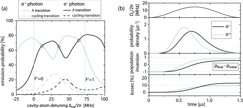
Figure 3: Polarised photons from a ⁸⁷Rb atom: (a) Photon emission probability as a function of the cavity-atom detuning $\Delta_{ca}$ with respect to the transition from $|0\rangle$ to $|e\rangle$. The ground state $F=1$ and the excited states $F^{\prime}=0$ and $F^{\prime}=1$ are incorporated in the simulation, as well as their spontaneous decay. The vertical grey lines indicate zero detuning to the transitions from $|F=1,m_{F}=0\rangle$ to $|F^{\prime}=0,m_{F^{\prime}}=0\rangle$ and $|F=1,m_{F}=0\rangle$ to $|F^{\prime}=1,m_{F^{\prime}}=0\rangle$, respectively. The probabilities for the generation of $\sigma^{+}$ and $\sigma^{-}$ photons are equal for three values of the detuning. They now deviate from a symmetrical picture with respect to the atomic resonances (grey vertical lines) since the transition amplitudes via both excited states interfere. (b) Time evolution of the system at $\Delta_{ca}/2\pi=63.2$ MHz: The probability density of the photon emission has a different shape for the emission of a $\sigma^{-}$ photon (black) and $\sigma^{+}$ photon (grey). The final population inversion of the atomic state differs from 1 because of losses due to spontaneous emission to $|F=2\rangle$ and $|F=1,m_{F}=0\rangle$. This leads to losses in the system which are about 10$\%$.

In Fig. 3 (a) the calculated emission probability is shown as a function of the cavity-atom detuning $\Delta_{ca}$, with the black lines again showing emission probabilities for $\sigma^{-}$ photons and grey lines for $\sigma^{+}$ photons. Compared to Fig. 2 (b), the symmetry around $\omega_{c}=\omega_{0e}$ is lost. At this frequency the probabilities for $\sigma^{+}$ and $\sigma^{-}$ photon emissions differ from one another although the cavity is in resonance with an atomic transition. This can be qualitatively understood because the influence of the $F^{\prime}=1$ state becomes larger the closer the virtual exited level is to this state. For a cavity-atom detuning of $\Delta_{ca}=0$, the virtual excited level is between $F^{\prime}=0$ and $F^{\prime}=1$ for the $\sigma^{+}$ process, but below the $F^{\prime}=0$ level for $\sigma^{-}$. Moreover, the detuning of the virtual level with respect to the atomic bare states determines the sign of the transition amplitudes. Therefore the two possible path of the Raman transition (via $F^{\prime}=0$ and $F^{\prime}=1$) interfere either constructively or destructively.

Although the former symmetry is lost, three cavity-atom detunings $\Delta_{ca}$ are found where the efficiencies for $\sigma^{+}$ and $\sigma^{-}$ photon production are equal. One is almost half-way between the two atomic resonances, and the other two are close to the $F=1$ to $F^{\prime}=0$ and $F=1$ to $F^{\prime}=1$ resonances. For the latter two cavity frequencies, the probability for generating a photon starting from the wrong initial state is below $7\%$ (Fig. 3 (a), dashed lines). This is an upper limit for the probability of generating a second photon after a first emission, if the process is started from the right initial state.

For instance, at $\Delta_{ca}/2\pi=63.2$ MHz, the equal probabilities for $\sigma^{+}$ and $\sigma^{-}$ photon emission reach a maximum of $74\%$. The time evolution of the system for this detuning is shown in Fig. 3 (b). The atom is exposed to the same pump pulse (shape and amplitude) for both directions of the Raman process. Although the probabilities for $\sigma^{+}$ and $\sigma^{-}$ photon emission are equal, the envelopes of the emitted photons differ, as can be seen in the probability-density plot. In fact, the virtual levels for the two transitions are not at the same energy and their transition amplitudes have different values. To produce identical photons, one could eventually compensate for this by choosing suitably shaped pump pulses for $\sigma^{+}$ and $\sigma^{-}$ processes. This is, however, beyond the scope of this article. Differences in the two processes can also be seen in the population transfer from the initial to the final state, see Fig. 3 (b). It is more successful for $\sigma^{+}$ photons, which indicates that the losses to non-coupled states are higher when a $\sigma^{-}$ photon is generated. Note that these losses never exceed $15\%$. Furthermore, from the low probability of the wrong transition to take place, we conclude that the starting conditions for a photon of opposite polarisation are always met once a first photon has been emitted. Therefore generating a sequence of photons of alternating polarisation seems feasible.

We have seen that the production of a photon when the atom is initially in the wrong Zeeman state is unlikely. We now show that one can address either the $|{\scriptstyle-}\rangle$ to $|{\scriptstyle+}\rangle$ or the $|{\scriptstyle+}\rangle$ to $|{\scriptstyle-}\rangle$ transition by choosing the appropriate pump laser frequencies. For a fixed cavity-atom detuning of $\Delta_{ca}/2\pi=63.2$ MHz, Fig. (4) shows the calculated emission probabilities as a function of the cavity-pump detuning, $\Delta_{cp}$. Again the pump laser Rabi frequency follows a pulse amplitude as shown in Fig. 3(b).

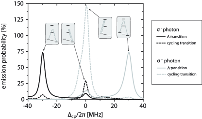
Figure 4: Dependency of the photon emission probability on the frequency difference of pump laser and cavity. The cavity-atom detuning is set to $\Delta_{ca}/2\pi=63.2$ MHz. The Raman resonance of laser and cavity at $\pm 2\Delta_{B}$ leads to sharp peaks in the photon emission probability for $\Lambda$ transitions while cycling processes are only visible around $\Delta_{cp}=0$.

As expected, we find maxima in the photon emission probability whenever Raman resonance conditions are met. Starting from state $|{\scriptstyle-}\rangle$, the emission probability for $\sigma^{-}$ photons shows a maximum at a pump laser detuning of $\Delta_{cp}=-30$ MHz, and similarly starting from state $|{\scriptstyle+}\rangle$ we find a maximum in the emission probability of $\sigma^{+}$ photons for $\Delta_{cp}=+30$ MHz. The emission probability amounts to $74\%$, as discussed before. Note that the Rayleigh scattering peak at $\Delta_{cp}=0$ dominates the spectrum. It exceeds 100% emission probability, since the pump laser hits the cavity resonance and the atom undergoes a cycling transition. For this reason, more than one photon per pulse can be emitted. These cycling transitions are more pronounced for $\sigma^{+}$ photons, since here the virtual excited level of the Raman transition is closer to a real atomic level. To guarantee single-photon emission in our scheme, transitions where two photons are possibly emitted have to be avoided. Since the width of the resonances depends on the cavity decay rate 2$\kappa$, the magnetic field has to be chosen high enough to ensure that the separation of the transition lines significantly exceeds 2$\kappa$. For the Zeeman splitting considered here the Raman resonances are well resolved and the scheme is not disturbed by cycling transitions, as can be seen in Fig. (4).

IV Conclusion

The calculations discussed in this paper are based on the parameters of an atom-cavity system that has been studied experimentally in our group Hennrich00 ; Kuhn02 ; Hennrich03 ; Legero04 . In these experiments, ⁸⁵Rb was used and the Raman transitions were driven between two different hyperfine ground states. The Zeeman structure of the levels was not important. Moreover, a repumping laser was necessary to re-establish the starting conditions after each photon emission. The scheme proposed here could easily be implemented if ⁸⁷Rb atoms were used and a magnetic field was applied. With the pump frequency being switched from one pulse to the next in a way that the Raman transition is either driven from $m_{F}=+1$ to $m_{F}=-1$ or vice versa, a stream of photons with alternating polarisation is expected. No time-consuming repumping will be needed, so that the photon-emission rate increases. The simulations show that equal efficiencies can be obtained for the production of $\sigma^{+}$ and $\sigma^{-}$ photons when an appropriate cavity-atom detuning is used. The efficiency is 74$\%$ for a cavity resonance close to the $F=1$ to $F^{\prime}=1$ transition frequency. The losses to other states are small, which guarantees that after a first emission the atom is well prepared to produce a subsequent photon. The realisation of this scheme seems promising. Since the produced photons have a well defined polarisation, they can be directed along arbitrary paths. This would be very convenient for quantum communication and all-optical quantum information processing in photonic networks Knill01 .

References

- (1) C. Cabrillo, J. I. Cirac, P. García-Fernández, and P. Zoller, Phys. Rev. A 59, 1025 (1999)
- (2) D. E. Browne, M. B. Plenio, and S.F. Huelga, Phys. Rev. Lett. 91, 067901 (2003)
- (3) L.-M. Duan, A. Kuzmich, and H. J. Kimble, Phys. Rev. A 67, 032305 (2003)
- (4) B. B. Blinov, D. L. Moehring, L.-M. Duan, and C. Monroe, Nature 428, 153 (2004)
- (5) S. Bose, P. L. Knight, M. B. Plenio, and V. Vedral, Phys. Rev. Lett. 85, 5158 (1999)
- (6) S. Lloyd, M. S. Shahriar, J. H. Shapiro, and P. R. Hemmer, Phys. Rev. Lett. 87428, 167903 (2001)
- (7) E. Knill, R. Laflamme, and G. J. Milburn, Nature 403, 515 (2001)
- (8) C. K. Hong, Z. Y. Ou, and L. Mandel, Phys. Rev. Lett. 59, 2044 (1987)
- (9) T. Legero, T. Wilk, A. Kuhn, and G. Rempe, Appl. Phys. B 77, 797 (2003)
- (10) A. Kuhn, M. Hennrich, and G. Rempe, Phys. Rev. Lett. 89, 067901 (2002)
- (11) M. Keller, B. Lange, K. Hayasaka, W. Lange, and H. Walther, Nature 431, 1075 (2004)
- (12) J. McKeever, A. Boca, A. D. Boozer, R. Miller, J. R. Buck, A. Kuzmich, and H. J. Kimble, Science 303, 1992 (2004)
- (13) M. Hennrich, T. Legero, A. Kuhn,and G. Rempe, Phys. Rev. Lett. 85, 4872 (2000)
- (14) M. Hennrich, A. Kuhn,and G. Rempe, J. Mod. Opt. 50, 935 (2003)
- (15) T. Legero, T. Wilk, M. Hennrich, G. Rempe, and A. Kuhn, Phys. Rev. Lett. 93, 070503 (2004)
- (16) M. O. Scully and M.S. Zubairy, Quantum optics (CambridgeUniversity Press, 1997)
- (17) A. Kuhn, M. Hennrich, T. Bondo, and G. Rempe, Appl. Phys. B 69, 373 (1999)
- (18) H. J. Metcalf and P. van der Straten, Laser cooling and trapping (Springer-Verlag New York, Inc., 1999)
- (19) D. A. Steck, Rubidium 87 D line data, Los Alamos National Laboratory, (2001, revised 2003)