Parallelism for Quantum Computation with Qudits

Abstract

Robust quantum computation with $d$-level quantum systems (qudits) poses two requirements: fast, parallel quantum gates and high fidelity two-qudit gates. We first describe how to implement parallel single qudit operations. It is by now well known that any single-qudit unitary can be decomposed into a sequence of Givens rotations on two-dimensional subspaces of the qudit state space. Using a coupling graph to represent physically allowed couplings between pairs of qudit states, we then show that the logical depth of the parallel gate sequence is equal to the height of an associated tree. The implementation of a given unitary can then optimize the tradeoff between gate time and resources used. These ideas are illustrated for qudits encoded in the ground hyperfine states of the atomic alkalies ⁸⁷Rb and ¹³³Cs. Second, we provide a protocol for implementing parallelized non-local two-qudit gates using the assistance of entangled qubit pairs. Because the entangled qubits can be prepared non-deterministically, this offers the possibility of high fidelity two-qudit gates.

I Introduction

Quantum computation requires the ability to process quantum data on a time scale that is small compared to the error rate induced by environmental interactions (decoherence). Robust computation results when the rate of error in the control operations and the rate of decoherence is below some threshold independent of the size of the computational register. The threshold theorem implies such rates exist, but it assumes arbitrary connectivity between subsystems as well as the ability to implement the control operations with a high degree of parallelism Preskill . Quantum computer architectures, therefore, should be designed to support parallel gate operations and measurements. At the software level some work has been done regarding parallel computation with qubits. For example, certain quantum algorithms such as the quantum Fourier transform can be parallelized Moore:98 , and there are techniques to compress the logical depth of a quantum circuit on qubits using the commutativity of gates in the Clifford group Raussendorf:02 . Further, by using distributed entanglement resources, some frequently used control operations can be parallelized Anocha:04 .

This work concerns parallel unitary operations on qudits, i.e. $d$ level systems where typically $d>2$. There are several reasons for considering such systems. Many physical candidates for quantum computation with qubits work by encoding in a subspace of a system with many more accessible levels. Control over all the levels is important for state preparation, simulating quantum processes, and measurement. In particular, encoding in decoherence-free subspaces usually involves control over multiple distinguishable states. Additionally, for small quantum computations, a fixed unitary $U\in U(d)$ for $d$ small but larger than $2$, can often be implemented with higher fidelity in a single qudit rather than by simulation with two-qubit gates. Further, at the level of tensor structures, some quantum processing may be more efficient with qudits, e.g. the Fourier transform over an abelian group whose order is not divisible by two Hoyer . It is straightforward to show that naïve qubit emulation of qudits is inefficient BOBII .

Fast single-qudit gate times are important in order to implement quantum error correction before errors accumulate Gottesman99 . In Section II we derive parallel implementations of general one-qudit unitary gates, where the quantum one-qudit gate library is restricted to a small set of couplings between two-dimensional subspaces (Givens rotations). The choice of this Givens library of one-qudit gates reflects standard coupling diagrams, i.e. the particular rotations obey selection rules in the physical system that encodes the qudit. Prior work considered minimum-gate circuits for such generalized coupling diagrams but did not further optimize these circuits in terms of depth selectionQR . Parallelism is possible because quantum gates on disjoint subspaces can be applied simultaneously, at the expense of additional control resources. Our method is particularly helpful for experimental implementations because it can be applied to a large class of systems with different allowed physical couplings. We provide examples for qudit control with ground electronic hyperfine levels of ⁸⁷Rb and ¹³³Cs and show that it is possible to achieve impressive speed-up with these systems using three pairs of control fields.

Further, in Section III we obtain depth-optimized (parallel) implementations of non-local two-qudit gates. Specifically, we describe how these operations, which generically require $O(d^{3})$ elementary two-qudit gates, can be parallelized to depth $O(d^{2})$ using $O(d^{3})$ maximally entangled qubit pairs (e-bits). While the protocol is not optimized in terms of e-bits consumed, it is a step forward to the goal of high fidelity two-qudit gates. The qubit resources can be chosen to be ancillary degrees of freedom of the particle encoding the qudit. Thus they can be prepared in entangled pairs non-deterministically and purified before the non-local gate is implemented.

A third aspect of parallelism Moore:98 involves reducing the logical depth of a circuit by judicious grouping of single- and two-particle gates that can be performed at the same time step, assuming connectivity of the particles. This is roughly analogous to classic circuit layouts and will not be considered here.

II Parallelism in state synthesis and unitary transformation for a single qudit

In typical physical systems encoding a single qudit, arbitrary couplings are not allowed. Whereas we can represent any unitary $U\in U(d)$ as an operator generated from an appropriate set of Hamiltonians, viz. $U=e^{-i\sum_{j=0}^{d^{2}}t_{j}h_{j}}$ where $t_{j}\in\mathbb{R}$ and $\sqrt{-1}h_{j}\in\mathfrak{u}(d)$ with $h_{j}=h_{j}^{\dagger}$, it is generally not possible to turn on all the couplings $h_{j}$ at the same time. It is a problem of quantum control to determine how to simulate a single-qudit unitary using a sequence of available couplings.

Because quantum computations need only be simulated up to a global phase, we restrict ourselves to implementations of a generic unitary $U\in SU(d)$. One way to a implement $U$ is by a covering with gates generated by the $\mathfrak{su}(2)$ subalgebras $\mathfrak{g}_{j,k}$ acting on the subspaces spanned by the state pairs $(|k\rangle,|j\rangle)$:

$$\begin{array}[]{lcll}\mathfrak{g}_{j,k}&=&\big{\{}\;i\lambda_{j,k}^{x,y,z}\;;&\lambda^{x}_{j,k}=|j\rangle\langle k|+|k\rangle\langle j|,\\ &&&\lambda^{y}_{j,k}=-i(|j\rangle\langle k|-|k\rangle\langle j|),\\ &&&\lambda^{z}_{j,k}=|j\rangle\langle j|-|k\rangle\langle k|\quad\quad\big{\}}\\ \end{array}$$ (1)

This is realized by a $QR$ decomposition of the inverse unitary into a product of unitary (Givens) rotation matrices that reduce it to diagonal form $D^{\dagger}$:

$$D^{\dagger}=\Big{[}\prod_{\ell=1}^{d(d-1)/2}G_{j_{\ell}k_{\ell}}\Big{]}U^{\dagger}.$$ (2)

Here, each Givens rotation can be chosen to be a function of two real parameters only:

$$G_{jk}(\gamma,\phi)=e^{-i\gamma(\cos\phi\lambda^{x}_{j,k}-\sin\phi\lambda^{y}_{j,k})}.$$ (3)

Typically, parameters are chosen so that consecutive Givens rotations introduce an additional zero below the diagonal of the unitary. Thus a sequence of such rotations realizes the inverse unitary up to relative phases, and the reversed sequence of inverse rotations realizes the unitary itself (up to a diagonal gate). There are $d(d-1)/2$ elements below the diagonal; hence the gate count in Eq. (2). The entire synthesis then follows by $U=D[\prod_{\ell=1}^{d(d-1)/2}G_{j_{\ell}k_{\ell}}]$. Using an Euler decomposition of $SU(2)$, the diagonal gate can be can be built using $3(d-1)$ Givens rotations.

A second way to synthesize a unitary transformation is to use a spectral decomposition

$$U=\prod_{\ell=0}^{d-1}W_{\ell}C_{\ell}W_{\ell}^{\dagger}$$ (4)

where $W_{\ell}$ is a unitary matrix that maps the basis state $|\ell\rangle$ to the eigenvector corresponding to the ${\ell}$th eigenvalue of $U$, and $C_{\ell}$ is the identity matrix with its $({\ell},{\ell})$ element replaced by the ${\ell}$th eigenvalue. Each matrix $W_{\ell}^{\dagger}$ implements a state-synthesis operation and can be implemented as a product of $G_{jk}(\gamma,\phi)$. The first major topic of this work is parallelism, both in state synthesis and in the two unitary constructions above.

Particular physical systems exhibit symmetries that constrain and refine the broad picture of unitary evolution presented so far MuthukrishnanStroud:00 ; Knill_state . This work focuses on systems in which a limited number of pairs of states can be coupled at any given time. The examplar system is a qudit encoded in the ground hyperfine state of a neutral alkali atom, where the number of pairs that may be coupled at once is determined by the number of lasers incident on the atoms. Other candidate systems for quantum computation, such as flux based Josephson junction qudits and electronic states of trapped ions, may allow this type of control.

We recall how selection rules on an atom with hyperfine electron structure constrains the allowed Givens evolutions of the system selectionQR ; spins . A pair of Raman pulses can couple states $|F_{\downarrow},M_{F}\rangle\leftrightarrow|F_{\uparrow},M_{F}^{\prime}\rangle$. In the linear Zeeman regime, a specific pair of hyperfine states can be addressed by choosing the appropriate frequency and polarization of the two Raman beams. The coupling acts on the electron degree of freedom which imposes a selection rule $\Delta M_{F}=M_{F}-M_{F}^{\prime}=\pm 2,\pm 1,0$. To demonstrate the power of our unitary synthesis technique, we restrict discussion to the selection rule $\Delta M_{F}=M_{F}-M_{F}^{\prime}=\pm 1,0$. This restriction is valid when the detuning of each Raman laser beam from the excited state is much larger than the hyperfine splitting in the excited state $(\Delta\gg E_{ehf})$ Deutsch:98 . There is a practical advantage to restricting discussion to this selection rule. Spontaneous emission during the Raman gate scales as $\gamma\sim\Gamma|\Omega_{1}\Omega_{2}|/\Delta^{2}$, where $\Omega_{1,2}$ are the Rabi frequencies of the two Raman beams and $\Gamma$ is the spontaneous emission rate from the excited state. Working in the limit of large detunings reduces errors due to spontaneous scattering events.

The hyperfine levels for a $d=8$ qudit and the induced coupling graph are shown in Figs. 1 and 2. We assume that the amplitude and phase of the Raman beams can be controlled so that each Givens rotation $G_{jk}(\gamma,\phi)$ can be generated in a single time step (see selectionQR ). It is notable that while the multitude of hyperfine levels in atomic systems provides a large state space of quantum information processing, these states are sensitive to errors. For instance, it is possible to choose disjoint two-dimensional subspaces, spanned by $\{|F_{\downarrow},M_{F}\rangle,|F_{\uparrow},-M_{F}\rangle\}$, that are insensitive to small magnetic field fluctuations along the quantization axis. Fluctuating fields along different axes have negligible effect provided a large enough fixed Zeeman field is applied. There are no such error avoidance codes when using the entire hyperfine. Hence parallelism, on a scale that can support error correction on a time scale fast compared to environmental noise, will be crucial.

II.1 Achieving parallelism in state synthesis

To implement the unitary state synthesis operator $W_{\ell}^{\dagger}$, we construct a sequence of rotations taking a particular vector to a given state $|\ell\rangle$. Again, this is technically the reverse of state synthesis:   $W|\ell\rangle=|\psi\rangle$ for a generic pure state $|\psi\rangle$ inverts to a sequence of unitaries $G_{jk}(\gamma,\phi)$ accomplishing $W^{\dagger}|\psi\rangle=|\ell\rangle$. Thus in the application $|\ell\rangle$ will be the fiducial state, and we attempt to treat all possibilities. We abbreviate the rotation of Eq. (3) by $G_{jk}$.

One tool for identifying sequences of rotations that produce $W_{\ell}^{\dagger}$ is the rotation or coupling graph, in which node $j$ is connected to node $k$ if a rotation between rows $j$ and $k$ is physically realizable qrrestricted . Then $W_{\ell}^{\dagger}$ is constructed by the sequence of rotations determined by constructing a spanning tree rooted at $\ell$ and successively eliminating leaf nodes by a rotation with their parent. Recall, a spanning tree of a graph $G(V,E)$ connects all $d=|V|$ nodes of $G$ with exactly $d-1$ edges from the set $E$.

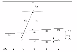
Figure 1: A single $d=8$ qudit encoded in the ground state hyperfine levels of ⁸⁷Rb. A pair of lasers can couple states in different hyperfine manifolds according to the selection rule $\Delta M_{F}=0,\pm 1$.

Figure 2: Coupling graph for ⁸⁷Rb.

Consider, for example, the coupling graph of Figure 2. To perform state synthesis for $|0\rangle$, we can form a spanning tree by breaking the edge between 1 and 5, breaking one of the edges in the cycle $0,5,2,4,1,6,0$, and choosing the root to be $|0\rangle$. If we break the edge between 2 and 4, then the resulting tree has three leaves, 7 (eliminated by $G_{07}$), 3 (eliminated by $G_{23}$). and 4 (eliminated by $G_{14}$), We can then eliminate the two resulting leaves 1 and 2, and then 6 and 5. Therefore, we have constructed a rotation sequence

$$G_{05}G_{06}G_{61}G_{52}G_{14}G_{23}G_{07}$$

that synthesizes $|0\rangle$ in 7 steps.

To understand the potential for parallelism, note that some of these rotations commute and can therefore be applied in parallel. This is a special case of the assertion that infinitesimal unitaries $ih_{1},ih_{2}\in\mathfrak{u}(d)$ may be applied in parallel iff $[h_{1},h_{2}]=0$ iff $e^{ith_{1}}$ and $e^{ith_{2}}$ commute for all $t$ real. We rely on the following result.

Proposition II.1

A subsequence of $p$ rotations can be applied in parallel if and only if all $2p$ indices are distinct.

Proof: It is easy to verify that if all four indices are distinct, then $G_{jk}G_{nm}=G_{nm}G_{jk}$. Conversely, if the four indices are not distinct, then the order of application matters and therefore the rotations cannot be applied in parallel. The result follows by induction on $p$. $\Box$

Using square brackets to group rotations that can be applied in parallel, the 7-step rotation sequence of our example becomes the 4-step parallel rotation sequence

$$G_{05}G_{06}[G_{61}G_{52}][G_{14}G_{23}G_{07}]\,.$$ (5)

The next interesting question is how we might determine an ordering of rotations to produce a parallel rotation sequence with a small number of steps. To answer this question, we build upon an algorithm of He and Yesha (heyesha, , Sec. 3.1). Given a spanning tree, they create a binary computation tree (BCT) by working from the bottom up and replacing every internal node in the spanning tree by a leaf connected to a chain of $p$ nodes, where $p$ is the number of children of the node. They then attach one child to each of the new nodes. The final result is a binary tree. (This process is illustrated in Figure 3 for a spanning tree of the coupling graph in Figure 2 rooted at node 3.) The following proposition shows that the number of steps in our parallel rotation sequence is equal to the height of the BCT, not the height of the spanning tree.

Proposition II.2

An ordering of the rotations can be obtained by constructing the BCT for a spanning tree of the coupling graph and scheduling each rotation at time step $k-j$, where $k$ is the height of the BCT and $j$ is the distance of the two leaves of the rotation from the root of the BCT. The resulting number of steps is $k-1$.

Proof: In constructing the BCT, we have split each node of the spanning tree that is involved in more than one rotation into a chain of nodes, each on a distinct level. This assures that rotations on the same level commute and therefore can be applied in parallel. $\Box$

The resulting ordering is within a factor of $O(\log_{2}m)$ of optimal, where $m$ is the number of rotations heyesha . We next present a direct (in fact greedy) algorithm which also orders the rotations for optimal parallelism.

At each step, consider each leaf of the spanning tree in order of its distance from the root (more distant leaves first), and process (remove) any leaf whose rotation can be applied in parallel with those already chosen for processing. The two algorithms give the same number of steps but perhaps assign a different timing to some rotations. For example, the greedy algorithm applied to the spanning tree on the left of Figure 3 yields

$$G_{32}G_{24}G_{25}[G_{50}G_{41}][G_{07}G_{16}]\,,$$

while the BCT on the right of the figure yields the schedule

$$G_{32}G_{24}[G_{25}G_{41}][G_{50}G_{16}]G_{07}.$$

Both rotation sequences require 5 steps.

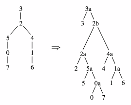
Figure 3: A spanning tree (left) and a BCT (right) for node 3 of ⁸⁷Rb.

Therefore, we can determine an ordering for the rotations to perform state synthesis for $|\ell\rangle$ by considering in turn each possible spanning tree rooted at $|\ell\rangle$, constructing an ordering for it, and choosing the ordering that provides the smallest number of steps.

It is possible that resource constraints prevent us from implementing a parallel ordering. Suppose for example a limited number of laser beams allows us to apply only two rotations at at time. State synthesis for $|0\rangle$ (Eq. 5) can still be accomplished using a 4-step rotation sequence, but it requires a nontrivial rearrangement:

$$G_{05}[G_{06}G_{52}][G_{61}G_{07}][G_{14}G_{23}]\,.$$ (6)

In general, such a constrained scheduling problem is difficult to solve exactly, although good heuristics exist.

II.2 Examples of parallelism in state synthesis

We apply our state synthesis algorithms to rubidium and cesium.

Hyperfine levels of ⁸⁷Rb.

Only the 9 transitions corresponding to the edges of the coupling graph of Figure 2 are allowed, and the edge between 1 and 5 will not be used in our algorithms, since it does not lead to speed-up footnote1 .

Optimal parallel rotation sequences, constructed using Proposition II.2, are given in Table 1. They require 5 steps for $|3\rangle$ and $|7\rangle$ and 4 steps for the other kets, rather than the 7 steps of the sequential algorithm.

Table 1: Parallel rotation sequences for state synthesis using laser Raman coupled connections between hyperfine states of ⁸⁷Rb.

$|0\rangle$	$G_{05}$ $[G_{06}G_{52}]$ $[G_{61}G_{07}]$ $[G_{14}G_{23}]$
$|1\rangle$	$G_{16}$ $[G_{60}G_{14}]$ $[G_{05}G_{42}]$ $[G_{23}G_{07}]$
$|2\rangle$	$G_{25}$ $[G_{24}G_{50}]$ $[G_{41}G_{23}]$ $[G_{16}G_{07}]$
$|3\rangle$	$G_{32}$ $G_{24}$ $G_{25}$ $[G_{50}G_{41}]$ $[G_{16}G_{07}]$
$|4\rangle$	$G_{41}$ $[G_{16}G_{42}]$ $[G_{25}G_{60}]$ $[G_{23}G_{07}]$
$|5\rangle$	$G_{50}$ $[G_{52}G_{07}]$ $[G_{06}G_{24}]$ $[G_{61}G_{23}]$
$|6\rangle$	$G_{61}$ $[G_{14}G_{60}]$ $[G_{05}G_{42}]$ $[G_{23}G_{07}]$
$|7\rangle$	$G_{70}$ $G_{06}$ $[G_{61}G_{05}]$ $[G_{14}G_{52}]$ $G_{23}$

Hyperfine levels of ¹³³Cs.

The coupling graph of allowed transitions for ¹³³Cs is given in Figure 4. We partition these transitions into three groups:

• The outer chain of (red) transitions between $|15\rangle$, $|0\rangle$, $|13\rangle$, $|2\rangle$, $|11\rangle$, $|4\rangle$, $|9\rangle$, $|6\rangle$, and $|7\rangle$.

• The inner chain of (blue) transitions between $|14\rangle$, $|1\rangle$, $|12\rangle$, $|3\rangle$, $|10\rangle$, $|5\rangle$, and $|8\rangle$.

• A ladder of transitions between the two chains.

Figure 4: Coupling graph for ¹³³Cs.

Since $d=16$, state synthesis requires 15 rotations. If the desired state is $|3\rangle$, for example, then we can use the outer chain of transitions to depopulate $|7\rangle$, $|6\rangle$, $|9\rangle$, $|4\rangle$ (in order) and then $|15\rangle$, $|0\rangle$, $|13\rangle$, $|2\rangle$, and then use the ladder transition from $|11\rangle$ to $|3\rangle$. Similarly, the inner chain of transitions can be used to empty $|14\rangle$, $|1\rangle$, $|12\rangle$, $|8\rangle$, $|5\rangle$, and finally $|10\rangle$. This pattern of using the outer chain, the inner chain, and a single ladder transition accomplishes state synthesis for an arbitrary state.

Complete parallelism is possible in the application of rotations from the outer chain with those in the inner, since no state is involved in both chains. If two rotations can be applied at once, then we need 9 steps for state synthesis to $|15\rangle$ or $|7\rangle$ and 8 steps for the other kets. We illustrate such a scheme in Figures 5 and 6, marking each transition with the step at which it is used.

Figure 5: State synthesis for $|1\rangle$ for the Cesium alkali using two-way parallelism. All transitions are directed toward $|1\rangle$.

II.3 Parallelism in one-qudit unitary processes

Recall that a state synthesis routine yields routines for realizing arbitrary one-qudit unitary evolutions in (at least) two different ways:   by invoking the $QR$ matrix decomposition (Eq. 2) or by the spectral theorem (Eq. 4). The number of parallel steps for a generic unitary can be significantly greater when using the spectral theorem. For example, for ⁸⁷Rb, the spectral decomposition would take 68 steps plus the steps needed to apply the phases. The number of steps to apply parallel $QR$ is much less; with 3-way parallelism it is at most $2n-3=13$ ($n=8$) plus the steps to apply the phases. Also note that the sequential $QR$ requires $n(n-1)/2=28$ steps, so this is a considerable speedup.

A rotation sequence that achieves this bound of 13 steps for $QR$ can be constructed using the precedence graph for the computation olst . Suppose we order the rows as $7,5,0,6,1,4,2,3$. We usually use rotations that eliminate an element in any row by a rotation with the element directly above it, but in the first column we use the rotation sequence

$$G_{70}G_{05}G_{06}[G_{52}G_{61}][G_{14}G_{23}].$$

This sequence specifies predecessors for each rotation in the first column. Define the predecessors of a rotation for columns after the first to be the rotations zeroing elements to the south, west and northwest, if those rotations exist. Each rotation can be performed after all of its predecessors are completed. Therefore, the numerical value of each entry below the diagonal in the following matrix denotes the step at which the entry can be zeroed:

$$\begin{array}[]{c}7\\ 5\\ 0\\ 6\\ 1\\ 4\\ 2\\ 3\end{array}\left[\begin{array}[]{r r r r r r r r}x&x&x&x&x&x&x&x\\ 4&x&x&x&x&x&x&x\\ 5&8&x&x&x&x&x&x\\ 3&7&9&x&x&x&x&x\\ 2&6&8&10&x&x&x&x\\ 1&5&7&9&11&x&x&x\\ 2&4&6&8&10&12&x&x\\ 1&3&5&7&9&11&13&x\\ \end{array}\right]\,.$$

Thus, using 3-way parallelism, an arbitrary unitary can be applied in 13 steps, plus the steps for phasing.

If only 2-way parallelism is allowed, then more steps are necessary. We schedule rotations by cycling through the columns in round-robin order (right to left), scheduling at most one rotation per column, until all rotations are scheduled. If the predecessors of the column’s next rotation are scheduled, then that rotation is scheduled for the earliest available time step after their scheduled steps. The resulting time steps are:

$$\begin{array}[]{c}7\\ 5\\ 0\\ 6\\ 1\\ 4\\ 2\\ 3\end{array}\left[\begin{array}[]{r r r r r r r r}x&x&x&x&x&x&x&x\\ 4&x&x&x&x&x&x&x\\ 6&10&x&x&x&x&x&x\\ 3&8&11&x&x&x&x&x\\ 2&7&9&12&x&x&x&x\\ 1&5&8&11&13&x&x&x\\ 2&4&6&9&12&14&x&x\\ 1&3&5&7&10&13&15&x\\ \end{array}\right]\,.$$

These $15$ steps are optimal for $2$-way parallelism; the last two rotations must be applied sequentially, so the $28$ rotations cannot be applied in $14$ steps.

Figure 6: State synthesis for $|7\rangle$ for the Cesium alkali using two-way parallelism.

A similar construction using the Cesium coupling graph shows that at most 29 steps are required using 7-way parallelism. We order the rows as 15,14,0,13,1,12,2,11,3,10,4,9,5,8,6,7. The rotations used in the first column are

$$\begin{array}[]{c}G_{15,0}G_{0,13}G_{13,2}G_{2,11}G_{11,4}G_{4,9}G_{9,5}G_{9,6}\\ $$[G_{0,14}G_{13,1}G_{2,12}G_{11,3}G_{4,10}G_{5,8}G_{6,7}],\end{array}$$

while in other columns we use rotations that eliminate an element in any row by a rotation with the element directly above it. The time steps are as follows:

$$\begin{array}[]{r}15\\ 14\\ 0\\ 13\\ 1\\ 12\\ 2\\ 11\\ 3\\ 10\\ 4\\ 9\\ 5\\ 8\\ 6\\ 7\end{array}\left[\begin{array}[]{r r r r r r r r r r r r r r r r}x&x&x&x&x&x&x&x&x&x&x&x&x&x&x&x\\ 1&x&x&x&x&x&x&x&x&x&x&x&x&x&x&x\\ 9&16&x&x&x&x&x&x&x&x&x&x&x&x&x&x\\ 8&15&17&x&x&x&x&x&x&x&x&x&x&x&x&x\\ 1&14&16&18&x&x&x&x&x&x&x&x&x&x&x&x\\ 1&13&15&17&19&x&x&x&x&x&x&x&x&x&x&x\\ 7&12&14&16&18&20&x&x&x&x&x&x&x&x&x&x\\ 6&11&13&15&17&19&21&x&x&x&x&x&x&x&x&x\\ 1&10&12&14&16&18&20&22&x&x&x&x&x&x&x&x\\ 1&9&11&13&15&17&19&21&23&x&x&x&x&x&x&x\\ 5&8&10&12&14&16&18&20&22&24&x&x&x&x&x&x\\ 4&7&9&11&13&15&17&19&21&23&25&x&x&x&x&x\\ 3&6&8&10&12&14&16&18&20&22&24&26&x&x&x&x\\ 1&5&7&9&11&13&15&17&19&21&23&25&27&x&x&x\\ 2&4&6&8&10&12&14&16&18&20&22&24&26&28&x&x\\ 1&3&5&7&9&11&13&15&17&19&21&23&25&27&29&x\\ \end{array}\right]$$

If fewer parallel resources are available, we can again reschedule our steps as done above for Rubidium. For 3-way parallelism, for example, we can schedule the rotations as

$$\begin{array}[]{r}15\\ 14\\ 0\\ 13\\ 1\\ 12\\ 2\\ 11\\ 3\\ 10\\ 4\\ 9\\ 5\\ 8\\ 6\\ 7\end{array}\left[\begin{array}[]{r r r r r r r r r r r r r r r r}x&x&x&x&x&x&x&x&x&x&x&x&x&x&x&x\\ 4&x&x&x&x&x&x&x&x&x&x&x&x&x&x&x\\ 19&24&x&x&x&x&x&x&x&x&x&x&x&x&x&x\\ 17&22&26&x&x&x&x&x&x&x&x&x&x&x&x&x\\ 3&19&24&28&x&x&x&x&x&x&x&x&x&x&x&x\\ 2&17&21&26&30&x&x&x&x&x&x&x&x&x&x&x\\ 11&15&19&23&28&32&x&x&x&x&x&x&x&x&x&x\\ 6&13&16&21&26&30&34&x&x&x&x&x&x&x&x&x\\ 2&11&14&18&23&28&32&35&x&x&x&x&x&x&x&x\\ 1&10&13&16&21&25&30&33&36&x&x&x&x&x&x&x\\ 5&8&11&14&18&23&27&31&35&37&x&x&x&x&x&x\\ 4&7&9&12&16&20&25&29&33&36&38&x&x&x&x&x\\ 3&6&8&10&14&18&22&27&31&34&37&39&x&x&x&x\\ 1&5&7&9&12&15&20&25&29&33&36&38&40&x&x&x\\ 2&4&6&8&10&13&17&22&27&31&34&37&39&41&x&x\\ 1&3&5&7&9&12&15&20&24&29&32&35&38&40&42&x\\ \end{array}\right]$$

Table 2: Number of parallel steps to synthesize a generic unitary operation $U$, up to a diagonal gate $D$, on a single atomic qudit. Each Raman pair of laser beams counts as a single resource and the logical depth is the number of parallel Raman gate sequences needed in our $QR$ diagonalization of $U$. The number in parenthesis is our best lower bound. The tradeoff between time and resources is evident.

Parallelism	Logical Depth: 87Rb (d=8)	133Cs (d=16)
7-way	$13$ (11)	$29$ (26)
6-way	$13$ (11)	$30$ (26)
5-way	$13$ (11)	$31$ (26)
4-way	$13$ (11)	$35$ (26)
3-way	$13$ (11)	$42$ (42)
2-way	$15$ (15)	$62$ (61)
1-way	$28$ (28)	$120$ (120)

A summary of the tradeoff between resources and gate times with qudits encoded in ground hyperfine levels of ⁸⁷Rb and ¹³³Cs is given in Table 2. As noted above, the 2-way construction of 15 steps for ⁸⁷Rb is optimal. Similar reasoning gives the 2- and 3-way lower bounds for ¹³³Cs; for example, 118 rotations divided by 3 gives 40 steps plus two final steps for the last two rotations. The other lower bounds in the table are obtained assuming a completely connected coupling graph and ($n/2$)-way parallelism. In that case, if $n=2^{p}$, we can insert $n/2$ zeros in the first column at step 1, up to $n/4$ zeros in the first two columns 2 at step 2, … , $1$ zero in the first $p$ columns at step $p$, and then start the reduction in the $j$th column for $j=p+1,\dots,n-1$ at step $\log_{2}n+2(j-\log_{2}n)$, for a total of $\log_{2}n+2(n-1-\log_{2}n)$ steps. Other choices of rotation sequences may reduce some entries in the table.

II.4 Parallel diagonal gates

Up to this point our discussion has counted the number of parallel steps needed to construct any single-qudit unitary up to a diagonal gate $D$. Synthesizing the diagonal gate is unnecessary if the target qudit will remain dormant until a measurement in the computational basis. However, if the qudit will be targetted by subsequent operations then it will be necessary to phase the basis states of the qudit appropriately. We next consider parallel constructions for $D$. There are two variations of this problem to discuss. In the first, we define a gate to be an evolution by the generator $\lambda_{j,k}^{z}$, where $j$ and $k$ are paired levels. In the second, the gate library is restricted to Givens rotations (Eq. 3) as is the case in systems controlled with Raman laser pairs. Here one cannot realize a diagonal Hamiltonian directly but rather may simulate $\mbox{e}^{it\lambda^{z}_{j,k}}$ using an Euler angle decomposition.

First, note that the $D$ gate itself need only be simulated up to a local phase: e.g., we may chose $D\in SU(d)$. Simulating a diagonal gate with $d-1$ independent phases should require appropriate couplings between $d-1$ pairs of states. There is a large amount of freedom in the choice of the set of the $d-1$ state pairs: any $D\in SU(d)$ can be written $D=\prod_{m=1}^{d-1}e^{i\phi_{j_{m},k_{m}}\lambda^{z}_{j_{m},k_{m}}}$, provided the set of edges $E=\{(j_{m},k_{m})\}$ creates a spanning tree of the coupling graph. For $\{i\lambda^{z}_{j,k}\;:\;(j,k)\in E\}$ spans the diagonal subalgebra of $\mathfrak{su}(d)$, and therefore we may construct $\{\phi_{j_{m},k_{m}}\}$ by solving $d-1$ linear equations selectionQR . Since diagonal gates commute, the simulation (in terms of $\lambda_{j,k}^{z}$) is maximally parallel, requiring one step. If only $k$-wise parallelism is allowed, then the number of steps is $\lceil(n-1)/k\rceil$.

We next consider the case that only $\lambda^{x}_{j,k}$ and $\lambda^{y}_{j,k}$ are allowed. Again choose any spanning tree for the coupling graph and construct $\{\phi_{j_{m},k_{m}}\}$ by solving $d-1$ linear equations. Color the edges of the tree so that no node has two edges of the same color. (For example, in Figure 3 we need 3 colors because node 2 has 3 edges.) Now for any edge $(j,k)$, we may indeed realize $\mbox{e}^{i\phi_{j,k}t\lambda^{z}_{j,k}}=\mbox{e}^{it_{1}(j,k)\lambda^{x}_{j,k}}\mbox{e}^{it_{2}(j,k)\lambda^{y}_{j,k}}\mbox{e}^{it_{3}(j,k)\lambda^{x}_{j,k}}$ for appropriate timings. Evolutions $\mbox{e}^{it_{1}\lambda_{j,k}^{x}}$ and $\mbox{e}^{it_{2}\lambda_{j,k}^{y}}$ do not commute and may not be applied in the same time step. Yet we may group the evolutions for a single color – black, for example – in three time steps as

$${\small\begin{array}[]{l}\big{[}\prod_{(j,k)\mbox{\footnotesize\ black}}\mbox{e}^{i\phi_{j,k}t_{1}(j,k)\lambda^{x}_{j,k}}\big{]}\big{[}\prod_{(j,k)\mbox{\footnotesize\ black}}\mbox{e}^{i\phi_{j,k}t_{2}(j,k)\lambda^{y}_{j,k}}\big{]}\\ \times\big{[}\prod_{(j,k)\mbox{\footnotesize\ black}}\mbox{e}^{i\phi_{j,k}t_{3}(j,k)\lambda^{x}_{j,k}}\big{]}\,.\end{array}}$$ (7)

Given a sufficient number of operations per step, this realizes $D$ in $3c$ parallel steps, where $c$ is the number of colors, regardless of the number of levels in the spanning tree. Hence, the construction is optimized by choosing a spanning tree that minimizes the number of colors. The number of colors $c$ is bounded by the maximum valency $c_{m}$ of any node in the coupling graph; if the coupling graph itself is a tree, then the number of colors is exactly $c_{m}$. When control resources are limited, we make a similar coloring, but limit the number of edges of a given color to the maximum number of operations allowed per step.

The spanning tree of Figure 3 for ⁸⁷Rb requires three colors for the edges. A diagonal computation can be done with the gate sequence $D=e^{i\phi_{3,2}\lambda^{z}_{3,2}}[e^{i\phi_{2,5}\lambda^{z}_{2,5}}e^{i\phi_{0,7}\lambda^{z}_{0,7}}e^{i\phi_{4,1}\lambda^{z}_{4,1}}][e^{i\phi_{5,0}\lambda^{z}_{5,0}}e^{i\phi_{2,4}\lambda^{z}_{2,4}}e^{i\phi_{1,6}\lambda^{z}_{1,6}}]$, which requires $9$ parallel Raman pulse sequences. Similarly, Cesium requires $9$ parallel Raman pulse sequences.

The above treatment works for synthesizing an arbitrary diagonal gate $D$ without prior processing. However, generically, the gate $D$ follows the diagonalization process process described in Sec. II.3. In that case some of pairwise phasing operations can be subsumed in earlier steps therefore reducing the total number of Raman pulse sequences. First, since Proposition II.1 can be extended to any unitary, not just rotations of the form $G_{jk}$, we can apply a phase correction using edge $(j,k)$ as soon as we are finished with those two rows in the diagonalization. Second, we are allowed to choose an edge set for phasing different than the one we used for diagonalization. For example, using 3-way parallelism for Rubidium, at times $11,12$, and $13$ of the diagonalization, we can apply a phase correction using edge $(0,6)$; at times $14$, $15$, and $16$ we can use $(7,0),(6,1)$, and $(5,2)$; and at times $17,18$, and $19$ we can finish by using $(0,5),(1,4)$, and $(2,3)$. A similar idea works for Cesium using 7-way parallelism: at times $27,28$, and $29$ use edge $(0,14)$; at times $30,31$, and $32$ use $(15,0),(14,1),(13,2),(12,3),(11,4),(10,5)$, and $(9,6)$; and at times $33,34$, and $35$ use $(0,13),(1,12),(2,11),(3,10),(4,9),(5,8)$, and $(6,7)$. In Rubidium, six extra Raman pulse sequences is optimal for phasing when nodes $|2\rangle$ and $|3\rangle$ are involved in the last rotation, and six pulses ending on $|6\rangle$ and $|7\rangle$ is optimal for Cesium. We require no more than three and six simultaneous couplings respectively, which is also the number required for optimal diagonalization.

III Parallelized non-local two-qudit gates

In this section we propose an implementation of an arbitrary non-local unitary $U\in U(d^{2})$ between two qudits $A$ and $B$. We suppose the qudits are spatially separated in some quantum computing architecture, yet this architecture has the capability to (i) prepare a large reservoir of maximally entangled ($d=2$) qubits and (ii) the ability to shuttle halves of such Bell pairs so that they are spatially close to qudits $A$ and $B$. Hence, part of the costing is the number of such Bell pairs (e-bits) consumed in the nonlocal gate. To be clear, we describe only a nonlocal two-qudit gate rather than a teleported two-qudit gate meaning that quantum operations are performed on two qudits rather than four. The optimization of such a nonlocal gate presented here arises by considering its component rotations in terms of the $QR$ decomposition.

Before stating the protocol, we argue for why it is needed. Two criteria must be satisfied to realize high performance two-qudit gates. First, nonlocality itself is desirable; most quantum computer architectures impose spatial limitations on inter-qudit couplings. It is very inconvenient to simply accept this limitation, since fault tolerant computation requires connectivity Oskin:02 . Now one might also suggest directly swapping qudits in order to achieve the required connectivity. Yet the swap gate itself may be faulty, and thus the resources required to make swapping fault tolerant might be prohibitive.

Second, reliable computation requires high fidelity two-qudit gates. Usually, Hamiltonians capable of entangling distinct qudits are difficult to engineer (at any fidelity) and would require effort to optimize for fidelity. Thus, one would likely choose a particular physically available entangling two-qudit Hamiltonian, e.g. perhaps the controlled-phase gate $P_{0}=e^{i\pi|0\rangle\langle 0|\otimes|0\rangle\langle 0|}$, and then exploit this with local unitary similarity transforms to achieve arbitrary Givens rotations between qudit levels. The entire process might simulate any $U\in U(d^{2})$ selectionQR . Local unitary similarity transforms arose naturally in this discussion, and it further implies that two-qudit nonlocality in such a scheme would follow, given a nonlocal protocol for a single entangling Hamiltonian.

It is difficult to design an architecture for two-qudit unitaries which allows for both high-fidelity and high connectivity. Some possibilities are noteworthy. As opposed to a chain of swapping operations, distant qudits might be swapped using entanglement resources. Then a non-local gate between qudits $A$ and $B$ can be done by teleporting $A$ to a location neighboring $B$, performing an entangling gate between $A$ and $B$ and teleporting back. Typically, entangled qudits (e-dits) rather than e-bits are used to teleport qudits; i.e. each teleportation is performed with the assistance of a maximally entangled two-qudit resource $|\Phi^{+}_{d}\rangle=\frac{1}{\sqrt{d}}\sum_{j=0}^{d-1}|j\rangle|j\rangle$ Bennett:93 . While the amount of entanglement consumed using the resource $|\Phi^{+}_{d}\rangle$ is low, i.e. one e-dit$=\log(d)$ e-bits, such a protocol would still require high fidelity (local) two-qudit gates between $A$ and $B$. As hinted at in the first paragraph of this section, a second alternative is to teleport the gate itself using an adaptation of the two-qubit gate teleportation protocol Gottesman ; Eisert (jozsa, , §2). In such an implementation one would build a generic two qudit gate between $A$ and $B$ using multiple applications of a gate teleport sequence where each sequence consumed two e-dits. Such a protocol would require the preparation of high fidelity e-dits and the implementation of generalized two-qudit Bell-measurements between a memory qudit and one half of an e-dit.

Here we describe a simple protocol for implementing a nonlocal two qudit gate, which has the advantage that one need only prepare high fidelity e-bits. If several qubits can be controlled together, the entire non-local gate can be parallelized to reduce the overall implementation time by a factor of $O(d)$.

III.1 A non-local controlled unitary gate

Consider a one-qudit unitary gate controlled on dit $(d-1)$:

$$\wedge_{1}(V)\ =\ \sum_{j=0}^{d-2}|j\rangle\langle j|\otimes{\bf 1}_{d}+|d-1\rangle\langle d-1|\otimes V\,.$$

We label the control qudit $A$ and the target qudit $B$. This subsection describes how such a gate can be implemented using

1. operators local to $A$ and $B$

2. an e-bit. The ancilliary e-bit is encoded in a pair of qubits, say $A_{1}$ and $B_{1}$, again with $A_{1}$ neighboring $A$ and $B_{1}$ neighboring $B$. The joint state of the ancilla is the Bell pair $|\Phi^{+}\rangle=(1/\sqrt{2})\;(|00\rangle+|11\rangle)_{A_{1},B_{1}}$.

3. a controlled-not gate controlled on the qudit and targeting an ancilliary qubit. As a formula, this gate is $\wedge_{1}(\sigma^{x})\ =\ \sum_{j=0}^{d-2}|j\rangle\langle j|\otimes{\bf 1}_{2}-|d-1\rangle\langle d-1|\otimes\sigma^{x}$.

4. a spatially local controlled $V$ gate with control an ancilla bit. As a formula, this is (also, confusingly) $\wedge_{1}(V)=|0\rangle\langle 0|\otimes{\bf 1}_{d}+|1\rangle\langle 1|\otimes V$.

The controlled gate of item 3 should be considered to be a primitive, highly engineered as discussed in the previous section. The controlled gate of item 4 might be decomposed into local gates and the gate of item 3 using standard techniques MuthukrishnanStroud:00 ; Knill_state ; selectionQR .

The procedure for realizing $\wedge_{1}(V)$ is as follows.

• Apply $\wedge_{1}(\sigma^{x}_{A_{1}})$ with $A$ as control and $A_{1}$ as target.

• Measure $({\bf 1}_{2}+\sigma^{z}_{A_{1}})/2$. Send the one bit (c-bit) classical measurement result, $m_{1}$, to the side of qudit $B$.

• Perform $e^{i\pi m_{1}\sigma^{x}_{B_{1}}/2}$ on the $B$ side of the architecture.

• Apply the operation $|0\rangle\langle 0|\otimes{\bf 1}_{d}+|1\rangle\langle 1|\otimes V$ with $B_{1}$ as control and $B$ as target.

• Measure $({\bf 1}_{2}+\sigma^{x}_{B_{1}})/2$ and send the c-bit measurement result $m_{2}$ to $A$.

• Apply the a relative phase to state $d-1$ of $A$ iff $m_{2}=1$, i.e. apply $P_{d-1}=e^{i\pi m_{2}|d-1\rangle_{A}{{}_{A}}\langle d-1|}$.

III.2 Bootstrap to nonlocal two-qudit state synthesis

We next consider the question of building a nonlocal two-qudit state synthesis operator. We may write any two-qudit state $|\psi\rangle=\sum_{j=0}^{d-1}|j\rangle\otimes|\psi_{j}\rangle$, where the kets $|\psi_{j}\rangle$ are unnormalized. We also take the convention that $W|\psi\rangle=|0\rangle$ so that $W^{\dagger}|0\rangle=|\psi\rangle$. Using the partition of the state vector, one may show that any two-qudit state-synthesis operator $W$ can be decomposed into $d-1$ elementary controlled-rotation operators as follows BOBII :

$$\begin{array}[]{lll}W&=&\ (V_{d}\otimes{\bf 1}_{d})\;\prod_{j=0}^{d-2}\Big{[}(F_{d-1-j}\otimes{\bf 1}_{d})\wedge_{1}(V_{d-1-j})\\ &&(F_{d-1-j}^{\dagger}\otimes{\bf 1}_{d})\Big{]}({\bf 1}_{d}\otimes V_{0})\,.\end{array}$$ (8)

Here we intend $F_{j}=|j\rangle\langle d-1|+|d-1\rangle\langle j|+\sum_{k\neq j,d-1}|k\rangle\langle k|$ to be a state-flip operator. The single-qudit operators $V_{j}$ are chosen so as to perform $V_{j}|\psi_{j}\rangle=t_{j}^{1/2}|0\rangle$, where $\langle\psi_{j}|\psi_{j}\rangle=t_{j}$ selectionQR . Then $V_{0}$ clears the remaining nonzero amplitudes.

The last subsection implicitly describes a non-local implementation of a controlled (one-qudit state synthesis) operator $W$, in that it details a scheme for the non-local $\wedge_{1}(V_{d-1-j})$. The resulting circuit for $W$ is shown in Fig. 7 and requires $d-1$ e-bits and $2(d-1)$ c-bits. Remarkably, the protocol can be parallelized to $7$ computational steps. Here by a single step we mean a set of operations that is no more time consuming than a controlled one qudit rotation $\wedge_{1}(V)$, which itself can be decomposed into controlled-phase gates and single qudit Givens rotations if so needed. The only nonobvious parallel step is step $4$. Note that the operators $V_{j}$ generally do not commute. However, just before and just after this step, the usual teleportation case study shows that the state of the system lies within the span of those $|k\rangle=|k_{0}\rangle_{A}\otimes_{j=1}^{d-1}|k_{j}\rangle_{B_{j}}\otimes|k_{d}\rangle_{B}$ in which at most a single $k_{j}$ is one for $1\leq j\leq d-1$. Let $P$ denote the projection of Hilbert space onto the span of all $|k\rangle$ as above. If $Q$ denotes the central product of Equation 8, we have

$$PQP\ =\ \prod_{j=1}^{d-1}e^{-it_{j}|1\rangle_{B_{j}}{{}_{B_{j}}}\langle 1|\otimes h_{j}}\\$$ (9)

For the map of Hamiltonians $h\mapsto PhP$ has image equal to the span of all $|1\rangle_{B_{j}}{{}_{B_{j}}}\langle 1|\otimes h$. Moreover, for $j_{1}\neq j_{2}$ and any Hermitian $h_{1},h_{2}$, we have $\big{[}\;|1\rangle_{B_{j_{1}}B_{j_{1}}}\langle 1|\otimes h_{1},|1\rangle_{B_{j_{2}}B_{j_{2}}}\langle 1|\otimes h_{2}\;\big{]}=0$. Hence we can generate the gates in step $4$ in parallel. The operations in step $5$ correspond to measurement of qubits $B_{j}$ in the Hadamard basis and count as a single parallel operation.

III.3 Spectral decomposition bootstrap to nonlocal gates

This protocol can be extended to implement an arbitrary non-local unitary $U\in U(d^{2})$ between $A$ and $B$. Consider the spectral decomposition Eq. (4) of $U$ which involves multiple applications of state-synthesis operators $W$ and controlled phase operators $C$. The controlled phase operators are locally equivalent to the operator $\wedge_{1}[{\bf 1}_{d}+(e^{i\phi}-1)|d-1\rangle\langle d-1|]$ and thus can be implemented in one step using one e-bit and two c-bits. Thus, any two-qudit unitary can then be built using $\ell=7\times 2d^{2}+d^{2}=15d^{2}$ parallel operations with the assistance of $\#_{e}=2\times(d-1)\times d^{2}+d^{2}=2d^{3}-d^{2}$ e-bits and $2\#_{e}$ c-bits.

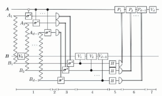
Figure 7: A non-local two qudit gate $U=W^{\dagger}$ that realizes the state-synthesis $U|0\rangle_{A,B}=|\psi\rangle_{A,B}$ on qudits $A$ and $B$ using $d-1$ ancillary qubit pairs (indicated by sawtooth lines) each prepared in the state $|\phi^{+}\rangle_{A_{j},B_{j}}=1/\sqrt{2}(|00\rangle+|11\rangle)_{A_{j},B_{j}}$. Each qubit $A_{j}(B_{j})$in the entangled resource can constitute a new particle or a distinct degree of freedom of qudit $A(B)$. Controlled-not gates between $A$ and $A_{j}$ are conditioned on the basis state $|j\rangle_{A}$, as indicated by the shading of the control bubble. The notations are: double lines for classical controlled operations dependent on qubit measurement outcomes, $H=e^{i\pi(\sigma^{x}+\sigma^{z})/2\sqrt{2}}$, and $P_{j}=e^{i\pi|j\rangle\langle j|}$. The sequence of steps that can be implemented in parallel is indicated at the bottom.

Recently, an alternative construction of two-qudit operations using qubit entanglement resources was proposed Zeng:05 . That work describes how a single e-bit and two c-bits suffice to implement a one parameter subgroup of $U(d^{2})$ between two distant qudits $A$ and $B$ with probability one. Specifically, their protocol realizes unitaries of the form $V(\phi)=\exp[i\phi U_{A}\otimes U_{B}]$ where the operators $U_{A},U_{B}$ are unitary and Hermitian. However, the authors do not provide an algorithm for generating an arbitrary two-qudit unitary nor do they estimate the number of e-bits consumed in a covering of $U(d^{2})$ with such unitaries.

III.4 Improved fidelity by purification

Our protocol requires local high fidelity operations between qudit $A$ and a set of qubits $\{A_{j}\}$ (similarly between $B$ and $\{B_{j}\}$) as well as high fidelity local unitaries. In principle, the entangling operations might be made error tolerant. Rather than use ancillary qubits that are distinct particles, we might use composite particles endowed a inherent tensor product structure $\mathcal{H}=\mathcal{H}_{\mbox{\footnotesize qudit}}\otimes\mathcal{H}_{\mbox{\footnotesize ancilla}}$ where one subsystem is used to encode the qudit and the ancillary subsystem is used to assist in two-qudit gate performance. Dür and Briegel Briegel showed that one can perform extremely high-fidelity two qubit gates with this partitioning. In their protocol, information is encoded in one two-dimensional degree of freedom of each particle, say spin. Entanglement between particles is generated using ancillary degrees of freedom such as quantized states of motion along $\hat{x},\hat{y}$ or $\hat{z}$. The prepared entanglement may not be perfect. Yet by using nested entanglement purification with two or more degrees of freedom, one can prepare a highly entangled state in the ancillary degrees of freedom with nonzero probability. If a purification round fails, then the entangled state can be reprepared without disturbing the quantum information encoded in the other degree of freedom (here spin). Given this, a non-local ${\rm CNOT}$ gate can be implemented between the encoded qubits.

Their protocol is readily extended to non-local gates between qudits using ancillary qubit degrees of freedom as discussed above. The critical assumption for robustness is that gates which couple different degrees of freedom of the same particle can be performed with much higher fidelity than gates which couple different particles. The assumption is frequently valid because coupling two spatially distinct particles usually involves interactions mediated by a field which can also couple to the environment and thus decohere the system. In contrast, gates between different degrees of freedom of the same particle, such as coupling spin to motion in trapped ions Sackett or atoms Haycock can often be implemented with high precision using coherent control.

IV Conclusions

Quantum computation with qudits requires more control at the single particle level than with qubits. It might be expected that the additional time needed to control all the levels would be prohibitively long in terms of memory decoherence times. We have shown how parallel (time-step optimized) one-qudit and two-qudit computation help surmount such difficulties. Given a qudit with a connected coupling graph, the time complexity for constructing an arbitrary unitary can be reduced at the expense of additional control resources. Even for systems with little connectivity between states, such as in the case of a qudit encoded in hyperfine levels of an atomic alkali, the number of parallel elementary gates can be made close to the optimal count for a maximally connected state space. For the purposes of two-qudit gates, we found a non-local implementation of an arbitrary unitary using $O(d^{2})$ parallel steps. The protocol uses $O(d^{3})$ e-bits which could be in principle be prepared and distributed ahead of time with high fidelity.

Some outstanding issues remain. First, our treatment focused on systems with allowed couplings between pairs of states. In other systems, the selection rules may dictate a different set of subalgebras to be used for quantum control, e.g. spin-$j$ representations of the algebra $\mathfrak{su}(2)$. Some particular computations may be realized with much greater efficiency using such generators. Second, fault tolerant computation relies not on exactly universal computation, but rather by approximating unitaries using a discrete set of one and two-qudit gates. It would be worthwhile to investigate optimal protocols for implementing a discrete set of fault tolerant non-local two qudit gates using entangled qubit pairs.

- (1) J. Preskill, Proc. R. Soc. London Ser. A 454, 385 (1998).
- (2) C. Moore and M. Nilsson, Parallel Quantum Computation and Quantum Codes, SIAM Journal on Computing 31, 799 (2001).
- (3) R. Raussendorf and H.-J. Briegel, Quant. Inf. and Comp. 6, 433 (2002).
- (4) A. Yimsiriwattana and S.J. Lomonaco, quant-ph/0403146.
- (5) P. Hoyer, quant-ph/9702028.
- (6) S. Bullock, D. O’Leary, and G. Brennen, Phys. Rev. Lett. 94, 230502 (2005).
- (7) D. Gottesman, Chaos, Solitons, and Fractals 10, 1749 (1999).
- (8) G. Brennen, D. O’Leary, and S. Bullock, Phys. Rev A 71, 052318 (2005).
- (9) A. Muthukrishnan and C.R.Stroud Jr., Phys. Rev. A 62, 052309 (2000).
- (10) E. Knill, http://www.arxiv.org/abs/quant-ph/9508006.
- (11) F. Albertini and D. D’Allesandro, Lin. Alg. App. 350 213 (2002).
- (12) I.H. Deutsch and P.S. Jessen, Phys. Rev. A 57, 1972 (1998).
- (13) D. P. O’Leary and S. S. Bullock, Electronic Transactions on Numerical Analysis, 21 20 (2005).
- (14) Xin He and Yaacov Yesha, Journal of Algorithms 9, 92 (1988).
- (15) Note that this transition corresponds to a . Selection rules for Raman laser pulses only allow this transition if both the pump and probe pulses are or polarized. Because this particular transition is not needed for parallelism we can fix the pump or probe pulse to have polarization and still access all the other couplings in the graph using frequency selectivity.
- (16) D. P. O’Leary and G. W. Stewart, Linear Algebra and Its Applications 77, 275 (1986).
- (17) M. Oskin, F.T. Chong, and I.L. Chuang, Computer, 35, 79 (2002).
- (18) C.H.Bennett, et al. Phys. Rev. Lett. 70, 1895 (1993).
- (19) D. Gottesman and I.L. Chuang, Nature 402, 390 (1999).
- (20) J. Eisert et al., Phys. Rev. A 62, 52317 (2000).
- (21) R.J. Jozsa, http://www.arxiv.org/abs/quant-ph/0508124 .
- (22) H.-S. Zeng, Y.-G. Shan, J-J Nie, and L.-M. Kuang, http://www.arxiv.org/abs/quant-ph/0508054.
- (23) W. Dür, H.-J. Briegel, Phys. Rev. Lett. 90, 067901 (2003).
- (24) C.A. Sackett et al., Nature, 404, 256 (2000).
- (25) D.J. Haycock et al., Phys. Rev. Lett. 85, 3365 (2000).