Binary projective measurement via linear optics and photon counting

Abstract

We investigate the implementation of binary projective measurements with linear optics. This problem can be viewed as a single-shot discrimination of two orthogonal pure quantum states. We show that any two orthogonal states can be perfectly discriminated using only linear optics, photon counting, coherent ancillary states, and feedforward. The statement holds in the asymptotic limit of large number of these physical resources.

Projection measurements play an essential role in photonic quantum-information protocols. In these applications, generally, a projection onto superposition states or entangled states of optical fields is required. Physically, it is a highly nontrivial problem how to implement such a measurement.

One plausible approach is to use linear optics and classical feedforward associated with a partial measurement. For example, a universal quantum computation scheme for photonic-qubit states has been proposed, which utilizes only linear optics, photon counting, and highly entangled auxiliary states of $n$ photons generated by probabilistic gate operations KLM01 . In principle, it works with unit success probability in the asymptotic limit of large $n$. It is, however, still a nontrivial question how to prepare entangled ancillae even for modest $n$.

In this paper, we discuss the linear optics implementation of a measurement which effects a projection onto two orthogonal states $\{|\Psi\rangle,|\Phi\rangle\}$. This is equivalent to the problem of discriminating two orthogonal quantum signals $\{|\Psi\rangle,|\Phi\rangle\}$ unambiguously vanLoock03 ; comment1 . We show that, in the asymptotic limit of a large number of partial measurements, one can perfectly discriminate the two states with linear optics, photon counting, and feedforward, but without any non-classical auxiliary states. Even in the worst case, the average error probability of discrimination approaches zero with the scaling factor of $N^{-1/3}$ where $N$ is the number of the partial measurements. Note that the signal space is two-dimensional but $|\Psi\rangle$ and $|\Phi\rangle$ can be any physical states defined in a larger space, e.g. qubit states, continuous variable states, etc.

Before discussing a linear optics implementation, it is worth mentioning a result concerning the distinguishability of two orthogonal multi-partite states via local operations and classical communication (LOCC). The necessary condition for exact local distinguishability is that, after doing a measurement at some local site, every possible remaining states must be orthogonal to each other. Walgate et al. Walgate00 showed that there always exists a local projective measurement satisfying this orthogonality condition for any set of two orthogonal states. Thus one can perfectly discriminate them via a series of local projective measurements where the choice of the measurement basis at each local site is conditioned on the previous measurement outcomes. This result means that if one can show a physical scheme that can exactly discriminate any two orthogonal single-mode states, its sequential application can achieve an exact discrimination of any two orthogonal multi-mode states. In the following, therefore, we concentrate on a discrimination of two single-mode states.

An arbitrary set of two orthogonal single-mode states are described by

$$|\Psi\rangle=\sum^{\infty}_{m=0}c_{m}|m\rangle_{0},\qquad|\Phi\rangle=\sum^{\infty}_{m=0}d_{m}|m\rangle_{0},$$ (1)

where $|m\rangle$ is an $m$-photon number state and $\langle\Psi|\Phi\rangle=\sum^{\infty}_{m=0}c_{m}^{*}d_{m}=0$. Figure 1 is the schematic of the measurement apparatus. The states are equally split into $N$ modes by $N-1$ asymmetric beamsplitters vanLoock00 ,

$$\hat{B}_{N-1,0}(\theta_{N-1})\hat{B}_{N-2,0}(\theta_{N-2})\cdots\hat{B}_{1,0}(\theta_{1})|0\rangle^{\otimes N-1}|\Psi\rangle_{0}$$

$$=e^{-\hat{a}_{N-1}^{\dagger}\hat{a}_{0}}\cdots e^{-\hat{a}_{1}^{\dagger}\hat{a}_{0}}e^{\hat{a}_{0}^{\dagger}\hat{a}_{0}\ln\left(1/\sqrt{N}\right)}|0\rangle^{\otimes N-1}|\Psi\rangle_{0}$$

$$\equiv\hat{N}_{BS}|\Psi\rangle_{0},$$ (2)

where $\hat{B}_{i,0}(\theta_{i})=\exp[\theta_{i}(\hat{a}^{\dagger}_{i}\hat{a}_{0}-\hat{a}_{i}\hat{a}^{\dagger}_{0})]$ Barnett97 and $\tan\theta_{i}=1/\sqrt{N-i}$. The input is symmetrically split to $N$ modes with the effective power reflectance of $1/N$. Then, at each output port, one makes some measurement by using linear optics and photon counters, where the information about the measurement outcome is fed forward to design the next measurement. It should be noted that this is a generalized version of the scheme so-called “Dolinar receiver” Dolinar73 ; Geremia04 ; Takeoka05 which was originally proposed as a physical model attaining the minimum error discrimination of the binary coherent signals $\{|\alpha\rangle,|-\alpha\rangle\}$.

We briefly sketch how two states are discriminated by such a scheme in the limit of $N\to\infty$ and then provide a rigorous proof. Suppose one inserts $|\Psi\rangle$ or $|\Phi\rangle$ into the first beamsplitter. For sufficiently small $1/N$, the reflectance of multi-photons can be neglected. The states after beamsplitting are approximated to be $\hat{B}_{1,0}(\theta_{1})|0\rangle_{1}|\Psi\rangle_{0}\approx|0\rangle_{1}|\eta_{0}\rangle_{0}+N^{-1/2}|1\rangle_{1}|\eta_{1}\rangle_{0}$, and $\hat{B}_{1,0}(\theta_{1})|0\rangle_{1}|\Phi\rangle_{0}\approx|0\rangle_{1}|\nu_{0}\rangle_{0}+N^{-1/2}|1\rangle_{1}|\nu_{1}\rangle_{0}$, where, $\langle\eta_{0}|\nu_{0}\rangle+\langle\eta_{1}|\nu_{1}\rangle/N\approx 0,$ since a beamsplitting operation is unitary. Then mode 1 is measured. The measurement here is required to maintain the orthogonality of any conditional outputs of $|\Psi\rangle$ and $|\Phi\rangle$. The local measurement satisfying this condition is described by a two-dimensional projective measurement,

$$|\pi_{0}\rangle = \mathcal{N}_{p0}\left\{|0\rangle+\frac{1}{X^{*}}\left(1-\sqrt{1+|X|^{2}}\right)|1\rangle\right\}$$ (3)

$$= \mathcal{N}_{p0}\left\{|0\rangle-(X+O(X^{2}))|1\rangle\right\},$$

$$|\pi_{1}\rangle = \mathcal{N}_{p1}\left\{(X^{*}+O(X^{2}))|0\rangle+|1\rangle\right\}.$$ (4)

where, $\mathcal{N}_{p0}$ and $\mathcal{N}_{p1}$ are the normalization factors and

$$X=\frac{2(\langle\nu_{0}|\eta_{1}\rangle\langle\eta_{1}|\nu_{1}\rangle-\langle\eta_{0}|\nu_{1}\rangle\langle\nu_{1}|\eta_{1}\rangle)}{\sqrt{N}(|\langle\eta_{0}|\nu_{1}\rangle|^{2}-|\langle\eta_{1}|\nu_{0}\rangle|^{2})}.$$ (5)

Here, we have assumed $|\langle\eta_{0}|\nu_{1}\rangle|^{2}-|\langle\eta_{1}|\nu_{0}\rangle|^{2}\neq 0$ which implies $X\propto 1/\sqrt{N}$ and thus we can take $|X|\ll 1$ in the limit of large $N$. The other case, i.e. $|\langle\eta_{0}|\nu_{1}\rangle|^{2}-|\langle\eta_{1}|\nu_{0}\rangle|^{2}=0$, will be discussed later. Under this assumption, the projective measurement of Eqs. (3) and (4) can be implemented by the displacement operation $\hat{D}(\beta_{1}/\sqrt{N})$ and photon counting as shown in Fig. 1(b). Since both the signal and displacement are sufficiently weak, the corresponding measurement vectors are described by

$$\hat{D}^{\dagger}\left(\frac{\beta_{1}}{\sqrt{N}}\right)|0\rangle \approx e^{-|\beta_{1}|^{2}/2N}\left(|0\rangle-\frac{\beta_{1}}{\sqrt{N}}|1\rangle\right),$$ (6)

$$\hat{D}^{\dagger}\left(\frac{\beta_{1}}{\sqrt{N}}\right)|1\rangle \approx e^{-|\beta_{1}|^{2}/2N}\left(\frac{\beta_{1}^{*}}{\sqrt{N}}|0\rangle+|1\rangle\right),$$ (7)

which can be same as Eqs. (3) and (4) by choosing appropriate $\beta_{1}$.

The conditional states after the first measurement can be rewritten again as $|\Psi^{\prime}\rangle=\sum^{\infty}_{m=0}c^{\prime}_{m}|m\rangle$ and $|\Phi^{\prime}\rangle=\sum^{\infty}_{m=0}d^{\prime}_{m}|m\rangle$. Since $\hat{N}_{BS}$ splits a state symmetrically, one can repeat the same procedure for the remaining state with the second beamsplitter, the displacement operation $\hat{D}(\beta_{2}/\sqrt{N})$, where $\beta_{2}$ is conditioned on the previous measurement outcome, and a photon counter. After repeating the same procedure to modes 1 to $N-1$ with appropriate $\beta_{i}$’s, the final states at mode 0 contain with dominating weight at most one photon and are still orthogonal to each other. As a consequence, applying the final ($N$-th) displacement and photon counting, one can exactly discriminate $|\Psi\rangle$ and $|\Phi\rangle$ with unit success probability.

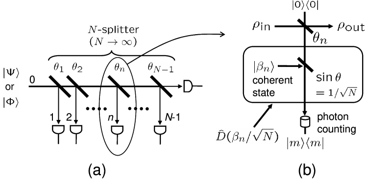
Figure 1: (a) $N$-splitter, and (b) a measurement apparatus at each step. A displacement operation $\hat{D}(\beta_{i}/\sqrt{N})$ is realized by combining the signal with a coherent state local oscillator $|\beta_{i}/\sqrt{N\sin\theta}\rangle$ via a beamsplitter with sufficiently small power reflectance of $\sin^{2}\theta$.

Now, we discuss the scheme rigorously, i.e. include the effects due to the multi-photon reflections at each beamsplitter, which contribute to the failure of the measurement or giving the incorrect decisions. Here, the input states $|\Psi\rangle$ and $|\Phi\rangle$ are always physical, that is, the average power of them are finite. Moreover, we assume that the probability distribution in photon number of those states decreases exponentially as $c_{m}\equiv\tilde{c}_{m}e^{-mx/2}$ where $x$ is a real positive number. The prior probabilities can be set to be equal without loss of generality. Finally we assume that the average powers of local oscillators always satisfy $|\beta_{i}|^{2}\leq|C_{\beta_{i}}|^{2}+O(1/N)$ where $C_{\beta_{i}}$ is a complex constant independent of $N$.

After finishing a whole process of $N$ measurement steps, one can classify the results according to the sequential patterns of detected photon numbers. Let us denote the events in which all the photon counters detect zero or one photon by ‘success’ events and the others by ‘failure’ events. Because of the symmetry of the $N$-beamsplitting, the probability of detecting $k$ photons at the $i$-th measurement on average over all possible measurement patterns is given by Barnett97

$$P_{k}^{(i)} = \left|{}_{i}\langle k|\hat{D}_{i}(\beta_{i}/\sqrt{N})\hat{N}_{BS}|\Psi\rangle_{0}\right|^{2}$$ (8)

$$\leq \frac{\langle\Psi_{\beta_{i}}|\hat{a}_{0}^{\dagger k}\hat{a}_{0}^{k}|\Psi_{\beta_{i}}\rangle}{N^{k}k!}+O\left(\frac{1}{N^{k+1}}\right)$$

$$\leq C_{k}^{\rm max}/N^{k}+O(1/N^{k+1}),$$

where $|\Psi_{\beta_{i}}\rangle\equiv\hat{D}(C_{\beta_{i}})|\Psi\rangle$, whose probability distribution still decreases exponentially in number basis (see Appendix A), and $C_{k}^{\rm max}$ is the maximum value of $\langle\Psi_{\beta_{i}}|\hat{a}_{0}^{\dagger k}\hat{a}_{0}^{k}|\Psi_{\beta_{i}}\rangle/k!$ for all $i$ and possible inputs C_k^max . The probability of resulting the failure event $P_{fail}$ is then bounded as

$$P_{fail} \leq (C_{2}^{\rm max}/N^{2}+O(1/N^{3}))\times N$$ (9)

$$= C_{2}^{\rm max}/N+O(1/N^{2}),$$

which implies that $P_{fail}$ approaches to zero in the limit of large $N$, at least with the order of $1/N$.

Even if the detection is successful, the conditional states get slightly non-orthogonal after each measurement step. To see this, we revisit the first beamsplitter $\hat{B}_{1,0}(\theta_{1})$. Let us describe the states after beamsplitting such that the orthogonal and non-orthogonal parts are separated as

$$\hat{B}_{1,0}(\theta_{1})|0\rangle|\Psi\rangle = |0\rangle|\eta_{0}\rangle+N^{-1/2}|1\rangle|\eta^{\prime}_{1}\rangle+N^{-1}|2\rangle|\eta_{2}\rangle+\cdots$$ (10)

$$= |0\rangle|\eta_{0}\rangle+N^{-1/2}|1\rangle|\eta_{1}\rangle+N^{-3/2}|1\rangle|\eta_{r}\rangle$$

$$+\sum_{k=2}^{\infty}N^{-k/2}|k\rangle|\eta_{k}\rangle,$$

$$\hat{B}_{1,0}(\theta_{1})|0\rangle|\Phi\rangle = |0\rangle|\nu_{0}\rangle+N^{-1/2}|1\rangle|\nu_{1}\rangle+N^{-3/2}|1\rangle|\nu_{r}\rangle$$ (11)

$$+\sum_{k=2}^{\infty}N^{-k/2}|k\rangle|\nu_{k}\rangle,$$

where the first two terms exactly satisfy the orthogonality $\langle\eta_{0}|\nu_{0}\rangle+\langle\eta_{1}|\nu_{1}\rangle/N=0$ and the last terms represent the multi-photon reflection terms. Here, $|\eta_{0}\rangle=\sum^{\infty}_{m=0}c_{m}(1-1/N)^{m/2}|m\rangle$, $N^{-1/2}|\eta^{\prime}_{1}\rangle=\sum^{\infty}_{m=1}c_{m}(m/N)^{1/2}(1-1/N)^{(m-1)/2}|m-1\rangle$, $N^{-1/2}|\eta_{1}\rangle=\sum^{\infty}_{m=1}c_{m}(1-(1-1/N)^{m})^{1/2}|m-1\rangle$, and $N^{-3/2}|\eta_{r}\rangle=N^{-1/2}(|\eta^{\prime}_{1}\rangle-|\eta_{1}\rangle)$ ($|\nu_{n}\rangle$’s are also obtained by replacing $c_{m}$ with $d_{m}$). The terms $|\eta_{r}\rangle$, $|\nu_{r}\rangle$ and that for multi-photon reflections, which have been neglected in the previous discussion, cause the residual non-orthogonality. Note that the leading terms of all vectors $|\eta_{k}\rangle$’s and $|\nu_{k}\rangle$’s are independent of $N$. Denote the $i$-th measurement operation as

$$\frac{{}_{i}\langle k|\hat{D}_{i}(\beta_{i}/\sqrt{N})\hat{B}_{i,0}(\theta_{i})|0\rangle_{i}|\Psi\rangle}{|{}_{i}\langle k|\hat{D}_{i}(\beta_{i}/\sqrt{N})\hat{B}_{i,0}(\theta_{i})|0\rangle_{i}|\Psi\rangle|}\equiv\hat{E}^{(i)}_{k}|\Psi\rangle.$$ (12)

Then the conditional outputs after detecting zero and one photons at the first measurement are given by

$$\hat{E}_{0}^{(1)}|\Psi\rangle = \mathcal{N}_{0}\left\{|\eta_{0}\rangle-\frac{\beta_{1}^{*}}{N}|\eta_{1}\rangle+\frac{1}{N^{2}}|\eta_{R_{0}}^{(1)}\rangle\right\},$$ (13)

$$\hat{E}_{1}^{(1)}|\Psi\rangle = \mathcal{N}_{1}\left\{\beta_{1}|\eta_{0}\rangle+|\eta_{1}\rangle+\frac{1}{N}|\eta_{R_{1}}^{(1)}\rangle\right\},$$ (14)

respectively, where $\mathcal{N}_{0}$ and $\mathcal{N}_{1}$ are the normalization factors and the third terms $|\eta_{R_{i}}^{(1)}\rangle$’s ($i=0,1$) come from $|\eta_{r}\rangle$ and $|\eta_{k}\rangle$’s for $k\geq 2$, and the terms in Eqs. (6) and (7) whose order is higher than $1/N^{1/2}$. The same outputs are obtained for $|\Phi\rangle$ by replacing $|\eta_{n}\rangle$ with $|\nu_{n}\rangle$. The first two terms in Eqs. (13) and (14) can be exactly orthogonal to those of $|\Phi\rangle$ by choosing $\beta_{1}/\sqrt{N}=(1-\sqrt{1+X^{2}})e^{i\omega}/X$, where X is obtained by substituting $|\eta_{0}\rangle$, $|\eta_{1}\rangle$, $|\nu_{0}\rangle$ and $|\nu_{1}\rangle$, appearing in Eqs. (10) and (11), into Eq. (5). Since $X\propto 1/\sqrt{N}$ as mentioned above, this choice of $\beta_{1}$ always satisfy the constraint on the average power of the local oscillator, $|\beta_{1}|^{2}\leq|C_{\beta_{1}}|^{2}+O(1/N)$. However, we have to care of the fact that, in both events, the total conditional states in Eqs. (13) and (14) are no longer orthogonal due to their third terms.

Now, suppose that the same strategy is applied to the choice of $\beta_{2}$ for the second measurement step. After the second measurement, the states are mapped into the new one with orthogonal and non-orthogonal terms, where the latter has two parts, i.e. contributions from the first and second measurements. Note that the leading order of prefactors of $|\eta_{R_{k}}^{(1)}\rangle$ with respect to $1/N$ does not change during the measurement process, as also the leading factors of $|\Psi\rangle$ does not change in the mapping in Eqs. (13) and (14). Eventually, after repeating $N-1$ measurement steps in a similar way, if all the photon counters detected zero or one photons, one obtains the conditional output consists of the orthogonal term and $N-1$ non-orthogonal terms stemmed from each measurement as

$$|\Psi^{(N-1)}\rangle = \hat{E}^{(N-1)}\cdots\hat{E}^{(1)}|\Psi\rangle$$

$$= |\eta^{(N-1)}\rangle+\frac{1}{N^{2}}\sum_{x=1}^{I^{(N-1)}}|H_{0}^{(i_{x})}\rangle+\frac{1}{N}\sum_{y=1}^{J^{(N-1)}}|H_{1}^{(j_{y})}\rangle,$$

where the first term is exactly orthogonal to that of $|\Phi^{(N-1)}\rangle$, while $|H_{k}^{(l)}\rangle$ is the residual non-orthogonal term coming from $|\eta_{R_{k}}^{(l)}\rangle$. $I^{(N-1)}$ and $J^{(N-1)}$ are the numbers of the events of detecting zero and one photon, respectively, and thus $I^{(N-1)}+J^{(N-1)}=N-1$.

Let us denote the final $N$-th measurement by $|D_{k}\rangle\equiv\hat{D}^{\dagger}(\beta_{N}/\sqrt{N})|k\rangle$ ($k=0,1$). Suppose that $\beta_{N}$ is designed such that $|D_{0}\rangle$ and $|D_{1}\rangle$ are the same as the orthogonal terms in $|\Psi^{(N-1)}\rangle$ and $|\Phi^{(N-1)}\rangle$, respectively, up to the order of $1/N^{1/2}$ (the higher order terms contribute to the detection error). Then the error probability $P_{err}^{D_{1}}=|\langle D_{1}|\Psi^{(N-1)}\rangle|^{2}$ is given by

$$P_{err}^{D_{1}} = \left|\sum_{x=1}^{I^{(N)}}\frac{\langle D_{1}|H_{0}^{(i_{x})}\rangle}{N^{2}}+\sum_{y=1}^{J^{(N)}}\frac{\langle D_{1}|H_{1}^{(j_{y})}\rangle}{N}\right|^{2}.$$ (16)

where $I^{(N)}+J^{(N)}=N$. The leading order of $\langle D_{1}|H_{k}^{(j)}\rangle$ is independent of $N$ for every $j$ and $k$.

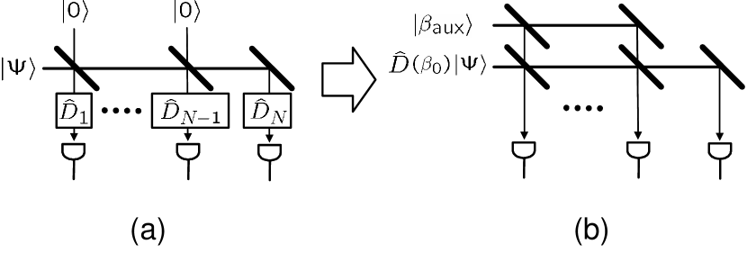
Figure 2: The original scheme (a) can be transformed into (b) where the total input photon number is the sum of those of two input states.

One can estimate the order of $J^{(N)}$ by counting the total amount of photons put into the system since the number of the total photon is equal to that of detectors. Although photons are supplied by the input state and $N$ displacements in the original configuration, one can simplify it into the one with only two inputs, $\hat{D}(\beta_{0})|\Psi\rangle$ and the coherent state $|\beta_{\rm aux}\rangle$, by adding some linear optics as illustrated in Fig. 2. Here, with the relation $\hat{D}_{A}(\alpha)\hat{D}_{B}(\beta)\hat{B}_{AB}(\theta)=\hat{B}_{AB}(\theta)\hat{D}_{A}(\alpha\cos\theta-\beta\sin\theta)\hat{D}_{B}(\alpha\sin\theta+\beta\cos\theta)$, one finds $|\beta_{0}|^{2}=|\sum_{i=1}^{N}\beta_{i}/N|^{2}$ and $|\beta_{\rm aux}|^{2}=\sum_{i=1}^{N}|\beta_{i}|^{2}/N-|\beta_{0}|^{2}$, where these are bounded as $|\beta_{0}|^{2}=C_{0}+O(1/N)$ and $|\beta_{\rm aux}|^{2}=C_{\rm aux}+O(1/N)$ due to the constraint on $|\beta_{i}|^{2}$’s. $C_{0}$ and $C_{\rm aux}$ are constants independent of $N$.

The probability of having $n$ photons in total is given by $P(n)=\sum_{m=0}^{n}P_{\rm sig}(n-m)P_{\rm aux}(m)=C_{P}e^{-nx}+O(1/N)$. Here the photon number statistics of two inputs, $P_{\rm sig}(m)$ and $P_{\rm aux}(m)$ are exponential and Poissonian, which easily implies that $P(n)$ decreases exponentially with resepect to $n$ (see Appendix C). Therefore, one can bound $J^{(N)}$ by some constant $C_{J}$ with exponentially small exception as

$${\rm Prob}\left[J^{(N)}\leq C_{J}+O(1/N)+N\epsilon\right]$$

$$\geq 1-C_{P}\exp[-(C_{J}+O(1/N)+N\epsilon)]+O(1/N)$$

$$=1-\tilde{C}_{P}e^{-N\epsilon}+O(1/N)$$ (17)

where $\epsilon$ can be arbitrarily small for large $N$. Eventually, substituting it and $I^{(N)}\leq N$ into Eq. (16), one obtains

$$P_{err}^{D_{1}} = \left|\frac{I^{(N)}}{N^{2}}\langle D_{1}|H_{0}\rangle_{\rm av}+\frac{J^{(N)}}{N}\langle D_{1}|H_{1}\rangle_{\rm av}\right|^{2}$$ (18)

$$\leq C_{E}/N^{2}+O(1/N^{3})+\epsilon O(1/N)+\epsilon^{2},$$

where $\langle D_{1}|H_{k}\rangle_{\rm av}=\sum_{i}\langle D_{1}|H_{k}^{(i)}\rangle/L$ ($L=I^{(N)}$ and $J^{(N)}$ for $k=0,\,1$, respectively), and $C_{E}$ is some constant independent of $N$. In a similar manner, the same bound is derived for $P_{err}^{D_{0}}=|\langle D_{0}|\Phi^{(N-1)}\rangle|^{2}$. Then, summing over all detection patterns, the average error probability is bounded as

$$P_{err}^{\rm tot} = \sum^{\rm success}P(\sharp)P^{succ}_{err}(\sharp)+\sum^{\rm failure}P(\sharp)P_{fail}(\sharp)$$ (19)

$$\leq \left(1-\frac{C_{2}^{\rm max}}{N}\right)\frac{P_{err}^{D_{0}}+P_{err}^{D_{1}}}{2}+\frac{C_{2}^{\rm max}}{N}+O\left(\frac{1}{N^{2}}\right)$$

$$\leq C/N+O(1/N^{2})+O(1/N)\epsilon+\epsilon^{2},$$

where $C$ is some constant and $P(\sharp)$ is the probability to observe the measurement sequence pattern $\sharp$. As a consequence, in the limit of $N\to\infty$, one can discriminate $|\Psi\rangle$ and $|\Phi\rangle$ with unit probability.

Finally, we discuss the case $|\langle\eta_{0}|\nu_{1}\rangle|^{2}-|\langle\eta_{1}|\nu_{0}\rangle|^{2}=0$ in Eq. (5), in which the desirable local measurement can not be implemented by a displacement and photon counting. Here, let us consider the projection measurement consisting of slightly perturbed vectors $|\Pi_{0}\rangle=\sqrt{1-\delta}|\Psi\rangle-\sqrt{\delta}|\Phi\rangle$ and $|\Pi_{1}\rangle=\sqrt{1-\delta}|\Phi\rangle+\sqrt{\delta}|\Psi\rangle$ with a perturbation parameter $\delta$. One can design such a measurement by the previous strategy with the total error probability of $P_{err}^{\rm tot}=C/N^{1-2\Delta}+O(1/N^{2-3\Delta})+O(1/N^{1-3\Delta/2})\epsilon+O(N^{\Delta})\epsilon^{2}$, where $\Delta=-\log_{N}\delta$. This device can discriminate the original states $|\Psi\rangle$ and $|\Phi\rangle$ with the average error probability of

$$P_{err}^{\rm av} = 1-(1-P_{err}^{\rm tot})(|\langle\Pi_{0}|\Psi\rangle|^{2}+|\langle\Pi_{1}|\Phi\rangle|^{2})/2$$ (20)

$$= C_{1}/N^{\Delta}+O(1/N^{2\Delta})+C_{2}/N^{1-2\Delta}+O(1/N^{2-3\Delta})$$

$$+O(1/N^{1-3\Delta/2})\epsilon+O(N^{\Delta})\epsilon^{2}$$

In the asymptotic limit of large $N$, this is minimized with $\Delta=1/3$ and then we obtain $P_{err}^{\rm av}=C/N^{1/3}+O(1/N^{2/3})+O(1/N^{1/2})\epsilon+O(N^{1/3})\epsilon^{2}$ which still converges to zero.

In summary, we have proved that arbitrary two orthogonal pure states can be perfectly discriminated by linear optics tools without using any non-classical ancillary states in the asymptotic limit of $N\to\infty$ where $N$ is the number of the detections and feedforwards. It implies that, in principle, one can implement arbitrary projection measurement in any two-dimensional signal space by these tools. The resources discussed here are mostly available with current technology. We also showed a concrete designing strategy of a linear optics circuit to attain this bound for a given $N$ and thus it can be directly applied for various quantum information protocols that require binary projection measurements. The remaining question is whether one can apply a same approach to the problem of more than three states discrimination.

We thank M. Ban, D. Berry, K. Tamaki, and P. van Loock for valuable discussions and comments. M.T. also acknowledges a kind hospitality at the QIT group in Universität Erlangen-Nürnberg. This work was supported by the DFG under the Emmy-Noether program, the EU FET network RAMBOQ and the network of competence QIP of the state of Bavaria.

Appendix A Photon number statistics of the displaced state

In this appendix, we show that if the photon number distribution of the initial state is exponential, then that of its displaced state is also bounded by exponentially decreasing function. For this purpose we use the following three formulae;

(1) The number basis components of the displacement operator Cahill69 ;

$$\langle n|\hat{D}(\xi)|m\rangle = \sqrt{\frac{m!}{n!}}\xi^{n-m}e^{-|\xi|^{2}/2}L_{m}^{(n-m)}(|\xi|^{2}),$$ (21)

for $(n\geq m)$ and

$$\langle n|\hat{D}(\xi)|m\rangle = \sqrt{\frac{n!}{m!}}(-\xi^{*})^{m-n}e^{-|\xi|^{2}/2}L_{n}^{(m-n)}(|\xi|^{2}),$$

for $(n\leq m)$, where $L_{n}^{(l)}(x)$ is the associated Laguerre polynomial defined by

$$L_{n}^{(l)}(x)=\sum_{k=0}^{n}{n+l\choose n-k}\frac{(-x)^{k}}{k!},$$ (23)

where $L_{n}^{(0)}(x)=L_{n}(x)$ is the Laguerre polynomial and

$$\frac{{\rm d}^{l}}{{\rm d}x^{l}}L_{n}(x)=(-1)^{l}L_{n-l}^{(l)}(x).$$ (24)

Proof. We basically follow the proof given in Barnett97 . To calculate $\langle n|\hat{D}(\xi)|m\rangle$, it is helpful to see $\langle n|\hat{D}(\xi)|n\rangle$, which is given by

$$\langle n|\hat{D}(\xi)|n\rangle = \langle n|\exp\left(\xi\hat{a}^{\dagger}-\xi^{*}\hat{a}\right)|n\rangle$$ (25)

$$= e^{-|\xi|^{2}/2}\langle n|e^{\xi\hat{a}^{\dagger}}e^{-\xi^{*}\hat{a}}|n\rangle$$

$$= \sum_{l=0}^{\infty}\sum_{m=0}^{\infty}e^{-|\xi|^{2}/2}\frac{\xi^{l}(-\xi^{*})^{m}}{l!m!}\langle n|\hat{a}^{\dagger\,l}\hat{a}^{m}|n\rangle$$

$$= \sum_{l=0}^{\infty}\sum_{m=0}^{\infty}e^{-|\xi|^{2}/2}\frac{\xi^{l}(-\xi^{*})^{m}}{l!m!}$$

$$\langle n-l|\sqrt{\frac{n!}{(n-l)!}}\sqrt{\frac{n!}{(n-m)!}}|n-m\rangle$$

$$= e^{-|\xi|^{2}/2}\sum_{m=0}^{n}{n\choose m}\frac{(-|\xi|^{2})^{m}}{m!}$$

$$= e^{-|\xi|^{2}/2}L_{n}(|\xi|^{2}).$$

Then we obtain

$$\langle n|\hat{D}(\xi)|n-l\rangle$$

$$=e^{-|\xi|^{2}/2}\langle n|e^{\xi\hat{a}^{\dagger}}e^{-\xi^{*}\hat{a}}\hat{a}^{l}|n\rangle\sqrt{\frac{(n-l)!}{n!}}$$

$$=e^{-|\xi|^{2}/2}\sqrt{\frac{(n-l)!}{n!}}\left(-\frac{\partial}{\partial\xi^{*}}\right)^{l}\langle n|e^{\xi\hat{a}^{\dagger}}e^{-\xi^{*}\hat{a}}|n\rangle$$

$$=e^{-|\xi|^{2}/2}\sqrt{\frac{(n-l)!}{n!}}(-\xi)^{l}\left(\frac{\partial}{\partial|\xi|^{2}}\right)^{l}L_{n}(|\xi|^{2}).$$ (26)

Therefore, replacing $n-l$ with $m$ in Eq. (A) with Eq. (24), we can derive Eq. (21).

(2) Bound on the associated Laguerre polynomials HandbookMath ;

$$\left|L_{n}^{(a)}(x)\right|\leq{a+n\choose n}e^{x/2},$$ (27)

where $x\geq 0$ and $a$ is an integer.

Proof. From Eq. (25), the absolute value of the Laguerre polynomial $L_{n}(x)$ with $x\geq 0$ is bounded by

$$|L_{n}(x)| = e^{x/2}\left|\langle n|\hat{D}(x^{1/2})|n\rangle\right|$$ (28)

$$\leq e^{x/2}.$$

To extend it to the associated Laguerre polynomial, we use the relation

$$L_{n}^{(a)}(x)=\sum_{k=0}^{n}{a+k-1\choose a-1}L_{n-k}(x),$$ (29)

which can be derived as

$$= \sum_{k=0}^{n}{a+k-1\choose a-1}\sum_{l=0}^{n-k}{n-k\choose l}\frac{(-x)^{l}}{l!}$$ (30)

$$= \sum_{l=0}^{n}\sum_{k=0}^{n-l}{a+k-1\choose a-1}{n-k\choose l}\frac{(-x)^{l}}{l!}$$

$$= \sum_{l=0}^{n}{n+a\choose n-l}\frac{(-x)^{l}}{l!}$$

$$= L_{n}^{(a)}(x),$$

where the formula

$$\sum_{k=0}^{n-l}{a+k\choose a}{n-k\choose l}={n+a+1\choose n-l}$$ (31)

has been utilized. Eventually, Eqs. (28), (29) and (31) imply

$$\left|L_{n}^{(a)}(x)\right| \leq \sum_{k=0}^{n}{a+k-1\choose a-1}\left|L_{n-k}(x)\right|$$

$$\leq \sum_{k=0}^{n}{a+k-1\choose a-1}e^{x/2}={a+n\choose a}e^{x/2}.$$

(3) Inequality for the binomial distribution GenIneq ;

$${n\choose\nu}y^{\nu}(1-y)^{n-\nu}\leq\exp\left[-2n(y-\nu/n)^{2}\right],$$ (33)

where $n>\nu$ and $0<y<1$.

Proof. Define $q=\nu/n$ and

$$f(y) = y^{\nu}(1-y)^{n-\nu}e^{-2n(x-q)^{2}},$$

$$F(y) = n^{-1}\ln f(x).$$ (34)

Then

$$F(y) = q\ln y+(1-q)\ln(1-x)+2(x-q)^{2},$$

$$F^{\prime}(y) = \frac{(q-y)(1-2y)^{2}}{y(1-y)},$$ (35)

and thus $F(y)$ takes its maximum at $y=q$. Also, the same for $f(y)$. Therefore, $f(y)\leq f(q)$, i.e.

$$y^{\nu}(1-y)^{n-\nu}e^{2n(y-q)^{2}}\leq q^{\nu}(1-q)^{n-\nu},$$ (36)

and thus

$${n\choose\nu}y^{\nu}(1-y)^{n-\nu}e^{2n(y-q)^{2}}\leq{n\choose\nu}q^{\nu}(1-q)^{n-\nu}\leq 1,$$ (37)

which completes the proof.

Derivation of the displaced state. Now we derive the main statement of this appendix. We assume that $|\Psi\rangle$ can be written as

$$|\Psi\rangle=\sum_{m=0}^{\infty}\tilde{c}_{m}e^{-mx/2}|m\rangle.$$ (38)

Now, let us calculate $\langle n|\hat{D}(\beta)|\Psi\rangle$.

$$\left|\langle n|\hat{D}(\beta)|\Psi\rangle\right|=\left|\sum_{m=0}^{\infty}\tilde{c}_{m}e^{-mx/2}\langle n|\hat{D}(\beta)|m\rangle\right|$$

$$\leq\sum_{m=0}^{\infty}\left|\tilde{c}_{m}e^{-mx/2}\langle n|\hat{D}(\beta)|m\rangle\right|$$

$$\leq\sum_{m=0}^{n}|\tilde{c}_{m}|e^{-mx/2}\left(\frac{m!}{n!}\right)^{1/2}|\beta|^{n-m}e^{-|\beta|^{2}/2}\left|L_{m}^{(n-m)}(|\beta|^{2})\right|+\sum_{m=n+1}^{\infty}|\tilde{c}_{m}|e^{-mx/2}\left(\frac{n!}{m!}\right)^{1/2}|\beta|^{m-n}e^{-|\beta|^{2}/2}\left|L_{n}^{(m-n)}(|\beta|^{2})\right|$$

$$\leq|\tilde{c}_{\rm max}|\sum_{m=0}^{n}e^{-mx/2}\left(\frac{m!}{n!}\right)^{1/2}|\beta|^{n-m}{n\choose m}+|\tilde{c}_{\rm max}|\sum_{m=n+1}^{\infty}e^{-mx/2}\left(\frac{n!}{m!}\right)^{1/2}|\beta|^{m-n}{m\choose n}$$

$$=|\tilde{c}_{\rm max}|\sum_{m=0}^{n}e^{-nx/2}\left\{{n\choose m}\frac{(|\beta|^{2}e^{x})^{n-m}}{(n-m)!}\right\}^{1/2}+|\tilde{c}_{\rm max}|\sum_{m=n+1}^{\infty}e^{-nx/2}\left\{{m\choose n}\frac{(|\beta|^{2}e^{-x})^{m-n}}{(m-n)!}\right\}^{1/2}$$

$$\leq\left\{ne^{-nx}|\tilde{c}_{\rm max}|^{2}\sum_{m=0}^{n}{n\choose m}\frac{(|\beta|^{2}e^{x})^{n-m}}{(n-m)!}\right\}^{1/2}+\left\{ne^{-nx}|\tilde{c}_{\rm max}|^{2}\sum_{m=n+1}^{\infty}{m\choose n}\frac{(|\beta|^{2}e^{-x})^{m-n}}{(m-n)!}\right\}^{1/2}.$$ (39)

The last line follows from the Cauchy-Schwarz inequality.

Introducing a real parameter $q$ which satisfies $e^{-x}<q<1$, the first term of Eq. (A) is then bounded as

$$\sqrt{n}e^{-nx/2}|\tilde{c}_{\rm max}|\left\{\sum_{m=0}^{n}{n\choose m}\frac{(|\beta|^{2}e^{x})^{n-m}}{(n-m)!}\right\}^{1/2}$$

$$=\sqrt{n}e^{-nx/2}|\tilde{c}_{\rm max}|\left\{\sum_{m=0}^{n}{n\choose m}q^{m}(1-q)^{n-m}\frac{1}{(n-m)!}\left(\frac{q|\beta|^{2}e^{x}}{1-q}\right)^{n-m}q^{-n}\right\}^{1/2}$$

$$\leq\sqrt{n}\left(\frac{e^{-x}}{q}\right)^{n/2}|\tilde{c}_{\rm max}|\left\{\sum_{m=0}^{n}{n\choose m}q^{m}(1-q)^{n-m}\exp\left[\frac{q|\beta|^{2}e^{x}}{1-q}\right]\right\}^{1/2}$$

$$=\sqrt{n}\left(\frac{e^{-x}}{q}\right)^{n/2}|\tilde{c}_{\rm max}|\exp\left[\frac{q|\beta|^{2}e^{x}}{2(1-q)}\right],$$

and thus it decreases exponentially as $n$ increases. Also, for the second term, one obtains

$$\sqrt{n}e^{-nx/2}|\tilde{c}_{\rm max}|\left\{\sum_{m=n+1}^{\infty}{m\choose n}\frac{(|\beta|^{2}e^{-x})^{m-n}}{(m-n)!}\right\}^{1/2}$$

$$=\sqrt{n}e^{-nx/2}|\tilde{c}_{\rm max}|\left\{\sum_{m=n+1}^{\infty}{m\choose n}q^{n}(1-q)^{m-n}\frac{1}{(m-n)!}\left(\frac{q|\beta|^{2}e^{-x}}{1-q}\right)^{m-n}q^{-n}\right\}^{1/2}$$

$$\leq\sqrt{n}\left(\frac{e^{-x}}{q}\right)^{n/2}|\tilde{c}_{\rm max}|\left\{\sum_{m=n+1}^{\infty}{m\choose n}q^{n}(1-q)^{m-n}\exp\left[\frac{q|\beta|^{2}e^{-x}}{1-q}\right]\right\}^{1/2}$$

$$\leq\sqrt{n}\left(\frac{e^{-x}}{q}\right)^{n/2}|\tilde{c}_{\rm max}|\exp\left[\frac{q|\beta|^{2}e^{-x}}{2(1-q)}\right]\left\{\sum_{m=n+1}^{\infty}\exp\left[-2m\left(q-\frac{n}{m}\right)^{2}\right]\right\}^{1/2}.$$

Since the last exponential term decreases exponentially as $m$ increase at least in the limit of $m\gg n$, the sum always converges within a finite value, which means that Eq. (A) itself also decreases exponentially as $n$ increases. As a consequence, these results imply that Eq. (A) decreases exponentially as $n$ increases.

Appendix B Derivation of the inequality (8)

In this appendix, we derive the inequality (8).

$$P_{k}^{(i)} = \left|{}_{i}\langle k|\hat{D}_{i}(\beta_{i}/\sqrt{N})\hat{N}_{BS}|\Psi\rangle_{0}\right|^{2}$$ (42)

$$= \left|{}_{i}\langle k|\hat{D}_{i}(\beta_{i}/\sqrt{N})\hat{B}_{N-1,0}(\theta_{N-1})\cdots\hat{B}_{i,0}(\theta_{i})\cdots\hat{B}_{1,0}(\theta_{1})|0\rangle^{\otimes N-1}|\Psi\rangle_{0}\right|^{2}$$

$$= \left|{}_{i}\langle k|\hat{D}_{i}(\beta_{i}/\sqrt{N})\hat{B}_{N-1,0}(\theta_{N-1})\cdots\hat{B}_{i+1,0}(\theta_{i+1})\hat{B}_{i-1,0}(\theta_{i})\cdots\hat{B}_{1,0}(\theta_{2})\hat{B}_{i,0}(\theta_{1})|0\rangle^{\otimes N-1}|\Psi\rangle_{0}\right|^{2}$$

$$= \left|{}_{i}\langle k|\hat{D}_{i}(\beta_{i}/\sqrt{N})\hat{B}_{i,0}(\theta_{1})|0\rangle_{i}|\Psi\rangle_{0}\right|^{2}$$

$$= \left|{}_{i}\langle k|e^{-|\beta_{i}|^{2}/2N}e^{\beta_{i}\hat{a}_{i}^{\dagger}/\sqrt{N}}e^{-\beta_{i}^{*}\hat{a}_{i}/\sqrt{N}}e^{-\hat{a}_{i}^{\dagger}\hat{a}_{0}\tan\theta_{1}}e^{-\ln\cos\theta_{1}(\hat{a}_{i}^{\dagger}\hat{a}_{i}-\hat{a}_{0}^{\dagger}\hat{a}_{0})}e^{\hat{a}_{i}\hat{a}_{0}^{\dagger}\tan\theta_{1}}|0\rangle_{i}|\Psi\rangle_{0}\right|^{2}$$

$$= \left|{}_{i}\langle k|e^{-|\beta_{i}|^{2}/2N}e^{\beta_{i}\hat{a}_{i}^{\dagger}/\sqrt{N}}e^{-\hat{a}_{i}^{\dagger}\hat{a}_{0}/\sqrt{N-1}}e^{\beta_{i}^{*}\hat{a}_{0}/\sqrt{N(N-1)}}e^{-\beta_{i}^{*}\hat{a}_{i}/\sqrt{N}}e^{\ln\sqrt{1-1/N}\hat{a}_{0}^{\dagger}\hat{a}_{0}}|0\rangle_{i}|\Psi\rangle_{0}\right|^{2}$$

$$= \left|e^{-|\beta_{i}|^{2}/2N}\left\{\sum_{j=0}^{k}{}_{i}\langle k-j|\frac{1}{j!}\sqrt{\frac{k!}{(k-j)!}}\left(\frac{\beta_{i}}{\sqrt{N}}-\frac{\hat{a}_{0}}{\sqrt{N-1}}\right)^{j}\right\}e^{\beta_{i}^{*}\hat{a}_{0}/\sqrt{N(N-1)}}e^{\ln\sqrt{1-1/N}\hat{a}_{0}^{\dagger}\hat{a}_{0}}|0\rangle_{i}|\Psi\rangle_{0}\right|^{2}$$

$$= \left|\frac{e^{-|\beta_{i}|^{2}/2N}}{\sqrt{k!}}e^{\hat{a}_{0}^{\dagger}\hat{a}_{0}\ln\sqrt{1-1/N}}\left(\frac{\beta_{i}-\hat{a}_{0}}{\sqrt{N}}\right)^{k}e^{\beta_{i}^{*}\hat{a}_{0}/N}|\Psi\rangle\right|^{2}$$

$$\leq \frac{\langle\Psi_{\beta}|\hat{a}_{0}^{\dagger k}\hat{a}_{0}^{k}|\Psi_{\beta}\rangle}{N^{k}k!}+O\left(\frac{1}{N^{k+1}}\right)$$

where $\cos\theta_{1}=\sqrt{1-1/N}$, $\sin\theta_{1}=1/\sqrt{N}$, $|\beta_{i}|^{2}\leq|C_{\beta_{i}}|^{2}+O(1/N)$ and $|\Psi_{\beta_{i}}\rangle=\hat{D}(C_{\beta_{i}})|\Psi\rangle$. We have used the relation $e^{\alpha\hat{a}_{j}}e^{\beta\hat{a}_{j}^{\dagger}}=e^{\beta\hat{a}_{j}^{\dagger}}e^{\alpha\hat{a}_{j}}e^{\alpha\beta}$ from line 5 to 6, and $e^{\phi\hat{a}_{j}^{\dagger}\hat{a}_{j}}\hat{a}_{j}e^{-\phi\hat{a}_{j}^{\dagger}\hat{a}_{j}}=\hat{a}_{j}e^{-\phi}$ from line 7 to 8, where $\alpha$, $\beta$, and $\phi$ are complex numbers. These relations are directly obtained from the commutation relation $[\hat{a}_{j},\hat{a}_{j}^{\dagger}]=1$.

The remaining task is to show that $\langle\Psi_{\beta_{i}}|\hat{a}^{\dagger\,k}\hat{a}^{k}|\Psi_{\beta_{i}}\rangle/k!$ is always finite, i.e.

$$\frac{\langle\Psi_{\beta_{i}}|\hat{a}^{\dagger\,k}\hat{a}^{k}|\Psi_{\beta_{i}}\rangle}{N^{k}k!}\leq\frac{C_{k}^{\rm max}}{N^{k}},$$ (43)

with a constant $C_{k}^{\rm max}$. Here, we replace $\beta_{i}$ by $\beta$ for simplicity. As shown in Appendix A, the photon number distribution of $|\Psi_{\beta}\rangle$ decreases exponentially. Denote

$$|\Psi_{\beta}\rangle\equiv\sum_{m=0}^{\infty}\tilde{b}_{m}e^{-mx/2}|m\rangle.$$ (44)

The absolute of complex coefficients $\tilde{b}_{m}$’s are always in between 0 and some constant due to the normalization constraint and let us denote the constant as $|\tilde{b_{\rm max}}|$. Then one has

$$\hat{a}^{k}|\Psi_{\beta}\rangle = \sum_{m=k}^{\infty}\tilde{b}_{m}e^{-mx/2}\sqrt{\frac{m!}{(m-k)!}}|m-k\rangle$$ (45)

$$= \sum_{m=0}^{\infty}\tilde{b}_{m+k}e^{-(m+k)x/2}\sqrt{\frac{(m+k)!}{m!}}|m\rangle,$$

and thus

$$\frac{\langle\Psi_{\beta}|\hat{a}^{\dagger\,k}\hat{a}^{k}|\Psi_{\beta}\rangle}{N^{k}k!} = \frac{e^{-kx}}{N^{k}k!}\sum_{m=0}^{\infty}|\tilde{b}_{m+k}|^{2}\frac{(m+k)!}{m!}e^{-mx}$$ (46)

$$\leq \frac{|\tilde{b}_{\rm max}|^{2}e^{-kx}}{N^{k}k!}\frac{k!}{(1-e^{-x})^{k+1}}$$

$$= \frac{1}{N^{k}}\frac{|\tilde{b}_{\rm max}|^{2}}{1-e^{-x}}\left(\frac{e^{-x}}{1-e^{-x}}\right)^{k}.$$

This bound depends on $\tilde{b}_{\rm max}$ and $x$ i.e. the state $|\Psi_{\beta_{i}}\rangle$. Therefore, maximizing the rhs of this inequality for all $|\Psi_{\beta_{i}}\rangle$ and denoting the maximum value as $C_{k}^{\rm max}/N^{k}$, one obtains Eq. (43).

Appendix C Total photon number statistics

The exponential and Poissonian distributions are described as

$$P_{E}(m)=C_{E}e^{-mx},$$ (47)

and

$$P_{P}(m)=\frac{C_{P}^{m}}{m!}e^{-C_{P}},$$ (48)

respectively. Then the distribution of the total photon number is given by

$$P_{\rm tot}(n) = \sum_{m=0}^{n}P_{P}(m)P_{E}(n-m)$$ (49)

$$= e^{-C_{P}}\sum_{m=0}^{n}\frac{C_{P}^{m}}{m!}C_{E}e^{-(n-m)x}$$

$$= C_{E}e^{-(C_{P}+nx)}\sum_{m=0}^{n}\frac{(C_{P}e^{x})^{m}}{m!}$$

$$\leq C_{E}e^{C_{P}(e^{x}-1)}e^{-nx},$$

which decreases exponentially as $n$ increases.

References

(1)
E. Knill, R. Laflamme, and G. J. Milburn,
Nature 409, 46 (2001).
(2)
P. van Loock and N. Lütkenhaus,
Phys. Rev. A 69, 012302 (2004).
(3)
This is true only for the case when all physical operations
during a whole measurement can be described by rank 1 operators.
As will be shown in the text, our scheme corresponds to this case.
(4)
J. Walgate, A. J. Short, L. Hardy, and V. Vedral,
Phys. Rev. Lett. 85, 4972 (2000).
(5)
P. van Loock and S. L. Braunstein,
Phys. Rev. Lett. 84, 3482 (2000).
(6)
has been used. See
S. M. Barnett and P. M. Radmore,
Methods in Theoretical Quantum Optics
(Oxford University Press, New York, 1997), for example.
(7)
S. J. Dolinar,
RLE, MIT, QPR No. 111, 1973 (unpublished) p. 115.
(8)
J. M. Geremia,
Phys. Rev. A 70, 062303 (2004).
(9)
M. Takeoka, M. Sasaki, P. van Loock, and N. Lütkenhaus,
Phys. Rev. A 71, 022318 (2005).
(10)
One can show that takes a finite value,
by using the exponential decay of the number distribution
of and the relation
.
(see Appendix B for details).
(11)
K. E. Cahill and R. J. Glauber,
Phys. Rev. 177, 1857 (1969).
(12)Handbook of Mathematical Functions, ed. M. Abramowitz
and I. A. Stegun (Dover Publications Inc., New York, 1965).
(13)General Inequalities 1, ed. E. F. Beckenbach
(Birkhäuser Verlag, Basel, 1978).