Matter-wave diffraction in time with a linear potential

Abstract

Diffraction in time of matter waves incident on a shutter which is removed at time $t=0$ is studied in the presence of a linear potential. The solution is also discussed in phase space in terms of the Wigner function. An alternative configuration relevant to current experiments where particles are released from a hard wall trap is also analyzed for single-particle states and for a Tonks-Girardeau gas.

,

1 Introduction

Diffraction in time (DIT) was studied first by Moshinsky [1, 2], and a flurry of both experimental and theoretical work investigating similar transient effects and setups have been carried out ever since. (For a brief, recent review see [3].) Quantum temporal oscillations of matter waves released from a shutter or confinement region constitute the hallmark of the effect.

Remarkably, all the theoretical studies have dealt with the quantum dynamics in free space or potentials with finite support [4, 5, 6]. However, the presence of a linear potential is ineludible for some experimental setups. This is actually the case for the first experimental observation of DIT, which made explicit use of gravity on a system of ultra cold atoms [7, 8]. Gravitational effects are also crucial in cold atom fountains as those used for frequency standards [9]. In addition, a linear potential arises from the interaction of a charged particle with an electric field, but it is within the field of atom optics that linear potentials, generally created by a magnetic field, have received a great deal of attention for ultracold atom manipulation, as a plugging potential for loading schemes, or aimed to cloud focusing, cooling, and other key operations [10, 11].

One of the natural configurations to deal with such situations in the stationary regime, namely that of a point-like and Gaussian sources, has already been discussed in excellent agreement with photo-detachment and atom-laser experiment [12]. In this work we generalize the Moshinsky shutter problem, i.e., a cut-off plane wave released at time $t=0$, by turning on a linear potential at that instant. The exact solution is derived in section 3 together with its Wigner function. A related configuration, namely, that of particles initially trapped in a rectangular box is analyzed in section 4. The experimental build up of all-optical hard-wall traps [13] has excited a great deal of attention for such geometries both at single [14, 15] and many-particle level [16, 17, 18, 19]. In particular, experiments are in view to study the quantum dynamics in the Tonks-Girardeau regime with Fock states of low particle number, $N$ [20]. The experimental observation of DIT with a Bose-Einstein condensate [21] is in excellent agreement with the dynamics entailed in the time-dependent Schrödinger equation, showing that the condensate evolves as a free non-interacting particle gas after few millisecond of expansion. Indeed, the importance of the non-linearity during free expansion has been studied in full detail for the case of a Tonks-Girardeau gas in [19] and shown to dominate in a time scale shorter than $t_{N}=mL^{2}/(2N\pi\hbar)$, $L$ being the size of the initial trap and $m$ the mass of the particle. The expansion of a Tonks-Girardeau gas will be analyzed in section 5.

2 Diffraction in time in free space

The paradigmatic setup for DIT corresponds to a beam of particles incident on a shutter represented by an infinite potential barrier. The relevance on the diffraction pattern of the reflectivity of the barrier [1] as well as different types of beam have been thoroughly investigated in [3]. For simplicity, we will assume here a totally absorbing barrier so that the initial state is given by a cut-off plane wave,

$$\psi(x,t=0)=e^{ipx/\hbar}\Theta(-x).$$ (1)

The solution to the time dependent Schrödinger equation [1, 2] reads

$$\psi(x,t)=M(x,p/\hbar,\hbar t/m):=\frac{e^{i\frac{mx^{2}}{2t\hbar}}}{2}w(-z),$$ (2)

with

$$z=\frac{1+i}{2}\sqrt{\frac{t}{m\hbar}}\left(p-\frac{mx}{t}\right),$$ (3)

and the so called Faddeyeva function [22, 23] $w$ is defined as

$$w(z):=e^{-z^{2}}{\rm{erfc}}(-iz)=\frac{1}{i\pi}\int_{\Gamma_{-}}du\frac{e^{-u^{2}}}{u-z},$$ (4)

where $\Gamma_{-}$ is a contour in the complex $z$-plane which goes from $-\infty$ to $\infty$ passing below the pole. After [24, 1], $M(x,k,t)$ has been named the Moshinsky function. The hallmark feature of this phenomenon is that, at variance with the classical solution, the probability density presents genuine quantum oscillations in time and space. Notice that a point of constant probability $P$ propagates as

$$x_{P}(t)=\frac{pt}{m}-\sqrt{\frac{\pi\hbar t}{m}}u_{0,P},$$ (5)

$u_{0,P}$ being a given constant. This result will be compared with the case where the evolution takes place in the presence of a linear potential.

3 Diffraction in time with a linear potential

We next study the DIT in the presence of a linear potential. Consider a beam of particles incident from the left as before on a totally absorbing shutter located at position $x=0$, see (1). Suddenly, the shutter is removed at time equal zero, and a linear potential is switched on. Such model can simulate the quantum dynamics of a confined charged particle, with a homogeneous electric field turned on at the time the infinite potential wall at the origin is removed. Also, it can be applied to a particle in a gravitational field; in that case the cut-off plane wave may be used as a basis element to describe the actual initial state.

The evolved wave function obeys the integral equation

$$\psi(x,t)=\int_{-\infty}^{\infty}dx^{\prime}K(x,t|x^{\prime},0)\psi(x^{\prime},0),$$ (6)

where $K(x,t|x^{\prime},t^{\prime})$ is the propagator for a Hamiltonian with a general linear potential of the form

$$\hat{H}=\frac{p^{2}}{2m}+fx,$$ (7)

with $f$ constant. It is indeed well known [25],

$$K(x,t|x^{\prime},t^{\prime})=\sqrt{\frac{m}{2\pi i\hbar(t-t^{\prime})}}\,e^{i\frac{m(x-x^{\prime})^{2}}{2\hbar(t-t^{\prime})}-i\frac{f(x+x^{\prime})(t-t^{\prime})}{2\hbar}-i\frac{f^{2}(t-t^{\prime})^{3}}{24\hbar}},$$ (8)

and related to the action of the classical path.

Inserting (8) into (6) we find

$$\psi(x,t)=\sqrt{\frac{m}{2\pi i\hbar t}}\,e^{-i\frac{f^{2}t^{3}}{24\hbar}-i\frac{ftx}{2\hbar}}\int_{-\infty}^{0}dx^{\prime}e^{i\frac{m(x-x^{\prime})^{2}}{2\hbar t}+i(p-ft/2)x^{\prime}/\hbar}.$$ (9)

It is convenient to introduce the auxiliary variables

$$u\equiv\sqrt{\frac{m}{\pi t\hbar}}(x^{\prime}-x)+\sqrt{\frac{t}{\pi m\hbar}}(p-ft/2),\\ u_{0}\equiv\sqrt{\frac{t}{\pi m\hbar}}(p-ft/2)-\sqrt{\frac{m}{\pi t\hbar}}x,$$ (10)

to write (9) as

$$\psi(x,t)=\frac{1}{\sqrt{2i}}\,e^{-i\frac{f^{2}t^{3}}{24\hbar}-i\frac{ftx}{2\hbar}}\int_{-\infty}^{u_{0}}due^{i\frac{\pi u^{2}}{2}},$$ (11)

which can be expressed in terms of the Fresnel sine and cosine integrals,

$$\int_{-\infty}^{u_{0}}du\,e^{i\frac{\pi u^{2}}{2}}=\frac{1+i}{2}+\int_{0}^{u_{0}}du\,e^{i\frac{\pi u^{2}}{2}}=\frac{1+i}{2}+C(u_{0})+iS(u_{0}).$$ (12)

From the last equation it is possible to map the probability density to the Cornu spiral [1]. Additionally, the following relation between the Fresnel integrals and the $w$-function holds [23],

$$C(u_{0})+iS(u_{0})=\frac{1+i}{2}\left(1-e^{i\frac{\pi u_{0}^{2}}{2}}w\left[\frac{\sqrt{\pi}}{2}(1+i)u_{0}\right]\right).$$ (13)

Then, one can make use of the Faddeyeva’s identity, which follows from the Cauchy theorem,

$$w(z)+w(-z)=2e^{-z^{2}},$$ (14)

to end up with the result

$$\psi(x,t) = \frac{1}{2}e^{-i\frac{f^{2}t^{3}}{24\hbar}-i\frac{ftx}{2\hbar}+i\frac{mx^{2}}{2m\hbar}}w(-z),$$ (15)

where now

$$z\equiv\frac{1+i}{2}\sqrt{\frac{t}{m\hbar}}\left(p-\frac{ft}{2}-\frac{mx}{t}\right).$$ (16)

In Fig. 1 a contour diagram of the probability density on the plane $t-x$ is plotted for a “fountain configuration”, namely, for the case in which the initial velocity goes in the direction of increasing potential. In such representation it is particularly easy to appreciate the diffraction in both time and space domains.

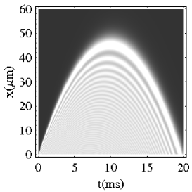
Figure 1: Probability density on the $t-x$ plane, which clearly shows the diffraction in time and space for an incident beam of Rubidium atoms in a fountain configuration ($p/m=1$ cm/s, $f/m=0.1*g$). The grey scale changes from light to dark as the function values decrease. The same color coding is used in all density plots.

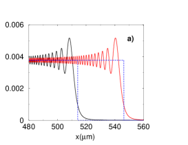
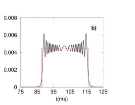
Figure 2: a) Probability density for both free an accelerated beam at $x>0$ with $p/m=5$ cm/s, $f/m=-0.1$ cm/s² (solid lines) and corresponding the classical density (dashed lines) $10$ ms after removing the shutter ($m=m_{Rb}$ in all the calculations).
b) Diffraction in time for an incident beam with $p/m=10$ cm/s registered by a detector located at $5$ mm from the shutter, $f/m=0.05$ cm/s². The dashed line corresponds to the classical density.

To learn about the main features of this solution, we compare it in Fig.2 with the free case. Indeed, it is amusing to rewrite (15) in terms of the Moshinsky function as

$$\psi(x,t)=e^{-i\frac{f^{2}t^{3}}{6m\hbar}+i\frac{ftx}{\hbar}}\,M\left(x-\frac{ft^{2}}{2m},\frac{p}{\hbar},\frac{\hbar t}{m}\right),$$ (17)

which exactly reduces to the result of section 2 for $f=0$. Notice that the dynamics is modified with respect to the free particle case by correcting both momentum and position with the classically expected time-dependent canonical transformation, as shown in Fig. 2a, up to an additional phase. In fact, the main difference is that, for a given $u$ the equation of motion for the associated point of constant probability, and in particular for the maximum and minimum, can be deduced to be

$$x_{max}(t) = \frac{pt}{m}-\frac{ft^{2}}{2m}-\sqrt{\frac{\pi\hbar t}{m}}u_{0,max},$$ (18)

$$x_{min}(t) = \frac{pt}{m}-\frac{ft^{2}}{2m}-\sqrt{\frac{\pi\hbar t}{m}}u_{0,min},$$ (19)

where $u_{max}=1.2172$ and $u_{min}=1.8725$ are universal for the cut-off plane wave case considered here. From these equations the turning point in Fig. 2 can be inferred.

As stated above, the telltale sign of DIT is a set of oscillations, observed after removing the shutter, in the probability density and which are genuinely quantum in nature. For diffraction in time with a linear potential, the fringe visibility

$$\mathcal{V}(T)=\frac{P_{1^{st}max}-P_{1^{st}min}}{P_{1^{st}max}+P_{1^{st}min}}$$ (20)

turns out to be independent of time, for the quasi-monochromatic case, as in the absence of the external field.

As pointed out before the diffraction in time admits also a representation of the Cornu spiral. The classical probability density, given by a step function, intersects the quantum one at two different points. Therefore, an estimate of the width for the largest fringe can be carried out by considering the intersection with the classical probability density. The same result than without linear potential holds,

$$\Delta x\simeq 0.85\sqrt{\frac{\pi\hbar t}{m}}$$ (21)

[1, 2] provided that the probability is exclusively $u$-dependent, as should be clear from (11), $P_{max}=1.370;P_{min}=0.778$. An alternative representation which explicitly exhibits the diffraction pattern in time domain is shown in Fig. 2b, where the position of the detector is fixed and the signal of the incident beam is recorded as a function of time. One should notice the similarity with the profile in coordinate representation obtained by releasing a particle from a hard-wall trap with $f=0$. This configuration was identified as the analogue of diffraction in time from a slit in free space [15]. Nevertheless, due to the dispersion entailed in (21) the pulse registered in the time domain is not symmetric.

3.1 Wigner transform

The Wigner function [26],

$$\mathcal{W}(x,p):=\frac{1}{\pi\hbar}\int_{-\infty}^{\infty}dy\,\psi(x+y)^{*}\psi(x-y)e^{2ipy/\hbar},$$ (22)

is the best known quasi joint probability distribution for position and momentum. Nowadays, it is possible to study it experimentally as has been demonstrated in a series of works [27]. In the context of the Moshinsky shutter, its time evolution was derived for the free case problem in [28]. From that result at $t=0^{+}$ or the definition (22), it follows that for the cut-off plane wave initial condition, the Wigner function reads

$$\mathcal{W}(x,p;p_{0},t=0^{+})=\frac{1}{\pi}\frac{\sin[-2x(p_{0}-p)/\hbar]}{p_{0}-p}\Theta(-x),$$ (23)

which clearly assumes negative values. For potentials of degree $n=2$ at most, the time evolved Wigner function follows the classical trajectories,

$$\mathcal{W}(x,p;t)=\int\!\!\!\int dx_{0}dp_{0}\delta[x-x_{cl}(x_{0},p_{0},t)]\delta[p-p_{cl}(x_{0},p_{0},t)]\mathcal{W}(x,p;t=0).$$ (24)

Alternatively one can cope with the more cumbersome calculation starting from the definition as in [28]. For (15) the result is

$$\mathcal{W}(x,p;p_{0},t)=\frac{\sin\bigg{\{}\frac{2}{\hbar}\left(\frac{pt}{m}+\frac{ft^{2}}{2m}-x\right)(p_{0}-ft-p)\bigg{\}}}{\pi(p_{0}-ft-p)}\Theta\left(\frac{pt}{m}+\frac{ft^{2}}{2m}-x\right).$$ (25)

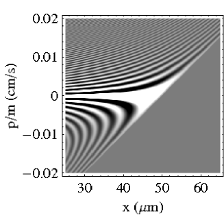
Figure 3: Wigner function for the atom fountain configuration at the classical turning point ($p_{0}/m=1$ cm/s, $f/m=100$ cm/s², $t=10$ ms). The grey triangle in the right lower corner is the classically unaccessible region for which $\mathcal{W}(x,p;t)=0$.

Fig. 3 shows the Wigner function calculated for an incident beam exactly at the classical turning point, being thus centered around $p=0$. Note that thanks to the step function, it is limited to the classically accessible region of the phase space. Indeed, following [28] we can ask for the classical limit taking $\hbar\rightarrow 0$ to find

$$\mathcal{W}_{cl}(x,p;p_{0},t)=\delta(p_{0}-ft-p)\Theta\left(\frac{p_{0}t}{m}-\frac{ft^{2}}{2m}-x\right).$$ (26)

As expected, the correct classical equation of motion ${x=x_{cl}(t),p=p_{cl}(t)}$ is recovered and no hint about the quantum oscillations -hallmark feature of DIT- remains.

4 The hard-wall trap

In this section we consider the dynamics of a particle initially confined in a box. At time zero its walls are suddenly removed and a linear potential is switched on. The paradigmatic particle in a box (PIAB) has been recently implemented in an all optical fashion by Raizen et al. [13] with a Bose-Einstein condensate and experiments are in view with Fock states of low number of particles, $N<10$ [20]. From the theoretical point of view, the free evolution of the wavefunction which results after shutting off the walls was discussed long time ago within the context of ultracold neutrons interferometry [14]. Later, it was reformulated by Godoy [15], who pointed out the analogy with the Fraunhoffer diffraction in the case of small box (compared to the De Broglie length), and Fresnel diffraction, for larger confinements. Quite recently , a generalization to an interacting many-body system was investigated in the regime of a Tonks-Girardeau gas [19].

If $\chi_{[0,L]}(z)$ is the characteristic function in the interval $[0,L]$, let us now consider the initial condition given by an arbitrary excited state $|\psi_{n}\rangle$,

$$\psi_{n}(x,t)=\sqrt{\frac{2}{L}}\sin\left(\frac{n\pi x}{L}\right)\chi_{[0,L]}(x).$$ (27)

Using the decomposition of the characteristic function $\chi_{[0,L]}(x)=\Theta(L-x)-\Theta(-x)$, the $\psi_{n}(x,t)$ term can be worked out to be

$$\psi_{n}(x,t) = \sqrt{\frac{m}{2\pi i\hbar t}}e^{-i\frac{ftx}{2\hbar}+i\frac{ft^{2}}{24\hbar}}$$ (28)

$$\times \sum_{\alpha=\pm}\alpha\left[\int_{-\infty}^{L}dx^{\prime}\,e^{i\frac{m(x-x^{\prime})^{2}}{2\hbar t}+i\frac{p_{\alpha}x^{\prime}}{2\hbar}}-\int_{-\infty}^{0}dx^{\prime}e^{i\frac{m(x-x^{\prime})^{2}}{2\hbar t}+i\frac{p_{\alpha}x^{\prime}}{\hbar}}\right],$$

where we have defined

$$p_{\alpha}\equiv\frac{\alpha\hbar n\pi}{L}-\frac{ft}{2}.$$ (29)

Carrying similar steps to the ones described for the previous section, one finally ends up with

$$\psi_{n}(x,t)=\frac{1}{4i}\sqrt{\frac{2}{L}}\,e^{-i\frac{ftx}{2\hbar}+i\frac{ft^{2}}{24\hbar}}\sum_{\alpha=\pm}\alpha\left[e^{i\frac{p_{\alpha}L}{\hbar}+i\frac{m(x-L)^{2}}{2\hbar t}}\,w(-u_{\alpha L})-e^{i\frac{mx^{2}}{2\hbar t}}\,\,w(-u_{\alpha 0})\right],$$ (30)

where

$$u_{\alpha L}=\frac{1+i}{2}\sqrt{\frac{t}{m\hbar}}\left(p_{\alpha}-\frac{m(x-L)}{t}\right),\,u_{\alpha 0}=\frac{1+i}{2}\sqrt{\frac{t}{m\hbar}}\left(p_{\alpha}-\frac{mx}{t}\right).$$ (31)

In an atomic fountain, trapped atoms are launched vertically with the help of the optical molasses technique. PIAB eigenstates are a good approximation to the actual state of a box subjected to a linear potential, whenever the box is small and the particle light. Indeed, within first order perturbation theory the coefficients $C_{nk}$ responsible for the corrections on the $n$-th eigenstate ($|\phi_{n}^{(1)}\rangle=|\phi_{n}^{(0)}\rangle+\sum_{k\neq n}C_{nk}|\phi_{k}^{(0)}\rangle$) due to the linear potential are given by

$$C_{nk}=\frac{8mfL^{3}}{\hbar^{2}\pi^{4}}\frac{nk[(-1)^{n+k}-1]}{k^{2}-n^{2}}.$$ (32)

If the perturbation of the initial state by the linear potential is significant, it can always be written as a linear combination of the eigenstates of the free Hamiltonian within the box, namely, $\{\phi_{n}(x)=\sqrt{2/L}\sin(n\pi x/L)|n\in{\bf N}\}$. We must therefore look for the evolution of a PIAB state released at time $t=0$ and launched with a given momentum $q$. Explicitly, it is described by (30), with the redefinition

$$p_{\alpha}\equiv q+\frac{\alpha\hbar n\pi}{L}-\frac{ft}{2}.$$ (33)

Equation (30) can model too the output coupling mechanism of an atom laser. In such devices, an atom is initially in the lasing mode, confined by the cavity mirrors which can be simulated by two infinite wall (reducing the problem to that of a PIAB). Through a Raman transition, this atom evolve to a nontrapped state, which amounts to shutting off the walls. During the transition and due to the emission of a photon the atom is kicked with a given momentum, namely, $q$ [29].

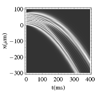
Figure 4: Time evolution of the density profile for an eigenstate of the hard-wall trap, with $n=10$, $q=0$ cm/s, $L=80$ $\mu$m and $f/m=0.49$ cm/s². Bifurcation for $t>t_{n=10}\simeq 137$ ms takes place in analogy with free case. The expectation value $\langle\hat{x}(t)\rangle$ reproduces the classical trajectory.

Figure 4 shows the time evolution of the density profile for the tenth eigenstate of the initial hard-wall trap. A most relevant feature is that at variance with the well-known harmonic trap case, the profile bifurcates into two main branches after the semiclassical time $t_{n}=mL/(2p_{n})=mL^{2}/(2n\pi\hbar)$. This behaviour has been recently reported for the free particle case by the authors [19] and holds for any excited state for both even and odd quantum number $n>1$. The cloud falls under acceleration following $\langle\psi|\hat{x}(t)|\psi\rangle$ the classical trajectory, even though for any $t>t_{n}$ the probability is vanishing along it.

5 Tonks gas dynamics in a linear potential

Under strong radial confinement and at low densities and temperatures an ultracold atomic gas becomes effectively one dimensional. In particular, whenever the thermal and zero-point energies are lower than the transversal excitation quantum, the Tonks-Girardeau (TG) regime is reached. The effective interactions are then so strong that the gas behaves like a system of hard-core impenetrable bosons. Such regime has been obtained in several experiments [30] and a full quantum description is possible thanks to the Fermi-Bose mapping theorem [31]. According to it, the many-body wavefunction of a TG gas can be obtained from the one of a zero-spin free fermionic gas, by applying the “antisymmetric unit function” $\mathcal{A}=\prod_{1\leq j<k\leq N}sgn(x_{k}-x_{j})$, as $\psi_{B}(x_{1},\dots,x_{N};t)=\mathcal{A}(x_{1},\dots,x_{N})\psi_{F}(x_{1},\dots,x_{N};t).$ Indeed one can state $|\psi_{B}(x_{1},\dots,x_{N};t)|^{2}=|\psi_{F}(x_{1},\dots,x_{N};t)|^{2}$, for the mapping is involutive. The dual system to the TG gas, being the ideal Fermi system, is built up as a Slater determinant

$$\psi_{F}(x_{1},\dots,x_{N};t)=\frac{1}{\sqrt{N!}}det_{n,k=1}^{N}\phi_{n}(x_{k};t).$$ (34)

Moreover, thanks to the fact that under unitary time evolution, orthonormality between the initial eigenstates of the trap is preserved, it follows that any local correlation function can be obtained in close-form. For example, the calculation of the density profile is greatly simplified to

$$\varrho(x,t)=N\!\!\int|\psi_{B}(x,x_{2},\dots,x_{N};t)|^{2}dx_{2}\cdots dx_{N}=\sum_{n=1}^{N}|\phi_{n}(x,t)|^{2}.$$ (35)

The free expansion dynamics of a TG gas from a hard-wall trap was recently considered in [19], where a dynamics much more complicated than for the harmonic confinement was observed. Taking advantage of the results obtained in the previous section we next generalize the free expansion results and deal with the following experiment. Consider a TG gas initially confined in a hard wall trap. At zero time it receives a momentum kick, momentum at which the shutter is off and the linear potential rumped up. The density profile is found combining (30) and (35).

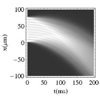
Figure 5: Time evolution of the density profile for Tonks-Girardeau gas , with $N=10$, $q=0$ cm/s, $L=80$ $\mu$m and $f/m=0.49$ cm/s². The interference pattern is washed out for $t>t_{N=10}\simeq 137$ ms.

Figure 5 shows the density profile of the expanding cloud in space and time falling under the action of a linear potential. For short times $t<t_{N}$ there is a well-defined pattern where the number of maxima equals that of particles. After a transient regime where the visibility of the peaks varies in a non-trivial way, it is gradually lost for $t>t_{N}$. In the later regime, the ballistic expansion is established in agreement with the force-free case [19].

6 Conclusions

Diffraction in time has been generalized in the presence of a linear potential. Moreover, the dynamics of particles released from a hard-wall trap under a constant force has been studied, showing a bifurcation after a time $t_{n}=mL^{2}/(2n\pi\hbar)$, in analogy with the free case [19]. This is a novel feature exclusively associated with hard-wall traps. Note that for the case of harmonic confinement, the evolution follows a scaling law of coordinates, lacking therefore any transient effect [33]. In addition, the expansion of a Tonks-Girardeau gas has been exactly solved using the Bose-Fermi map. The cloud is shown to exhibit an interference pattern which is lost for $t>t_{N}$. Finally, we point out that any time dependence on the linear potential can be easily included using the general map obtained in [34]. In such a way, one can account for a smooth ramping up of the linear potential.

References

References

- [1] Moshinsky M 1952 Phys. Rev. 88 625
- [2] Moshinsky M 1976 Am. Jour. Phys. 44 1037
- [3] del Campo A and Muga J G 2005 J. Phys. A 38 9803
- [4] Kleber M 1994 Phys. Rep. 236 331
- [5] García-Calderón G and Rubio A 1997 Phys. Rev. A 55 3361
- [6] García-Calderón G and Villavicencio J 2001 Phys. Rev. A 64 012107
- [7] Steane A, Szriftgiser P, Desbiolles P and Dalibard J 1995 Phys. Rev. Lett. 74 4972
- [8] Arndt A, Szriftgiser P, Dalibard J and Steane A M 1996 Phys. Rev. A 53 3369
- [9] Clairon A, Laurent P, Nadir A, Drewsen M, Grison D, Lounis B and Salomon C 1992 EFTF: Proceedings of 6th European Frequency and Time Forum
- [10] Folman R, Krüger P and Schmiedmayer J 2002 Adv. Atom. Mol. Opt. Phys. 48 263
- [11] Metcalf H J and van der Straten P 1999 Laser Coooling and Trapping (New York: Springer)
- [12] Kramer T, Bracher C and Kleber M 2002 J. Phys. A 35 8361; Kramer T 2003 Matter waves from localized sources in homogeneous force fields http://tumb1.biblio.tu-muenchen.de/publ/diss/ph/2003/kramer.pdf and reference therein
- [13] Meyrath T P, Schreck F, Hanssen J L, Chuu C-S. and Raizen M G 2005 Phys. Rev. A R71 041604
- [14] Gerasimov A S and Kazarnovskii M V 1976 Sov. Phys. JETP 44 892
- [15] Godoy S 2002 Phys. Rev. A 65 042111
- [16] Gaudin M 1971 Phys. Rev. A 4 386
- [17] Cazalilla M A 2002 Europhys. Lett. 59 793; Cazalilla M A 2004 J. Phys. B 37 S1
- [18] Batchelor M T, Guan X W, Oelkers N and Lee C 2005 J. Phys. A 38 7787
- [19] del Campo A and Muga J G 2005 cond-mat/0511747
- [20] Raizen M G 2005 Personal communications
- [21] Colombe Y, Mercier B, Perrin H and Lorent V 2005 Phys. Rev. A 72 061601
- [22] Faddeyeva V N and Terentev N M 1961 Mathematical Tables: Tables of the values of the function for complex argument (New York: Pergamon)
- [23] Abramowitz A and Stegun I A 1965 Handbook of Mathematical Functions (New York: Dover)
- [24] Moshinsky M 1951 Phys. Rev. A 84 525
- [25] Grosche C and Steiner F 1998 Handbook of Feynman path integrals, 145 Springer Tracts in Modern Physics (Berlin: Springer)
- [26] Wigner E P 1932 Phys. Rev. 40 749
- [27] Smithey D T et al 1993 Phys. Rev. Lett. 70 1244; Leibfried D et al 1996 Phys. Rev. Lett. 77 4281; Breitenbach G, Schiller S and Mlynek J 1997 Nature 387 471; Kurtsiefer Ch, Pfau T and Mlynek J 1997 Nature 386 150; Lvovsky A I et al 2001 Phys. Rev. Lett. 87 050402; Lougovski P et al 2003 Phys. Rev. Lett. 91 010401
- [28] Mánko V, Moshinsky M and Sharma A 1999 Phys. Rev. A 59 1809
- [29] Hagley E W et al 1999 Science 283 1706
- [30] Paredes B et al 2004 Nature (London) 429 227; Kinoshita T, Wenger T and Weiss D 2004 Science 305 1125
- [31] Girardeau M 1960 J. Math. Phys. 1 516
- [32] Brouard S and Muga J G 1996 Phys. Rev. A 54 3055
- [33] Perelomov A M and Zel’dovich Y B 1998 Quantum mechanics: selected topics, (Singapore:World Scientific)
- [34] Song D Y 2003 Europhys. Lett. 65 622