Elastic vs. inelastic coherent backscattering of laser light by cold atoms:
a master equation treatment

Abstract

We give a detailed derivation of the master equation description of the coherent backscattering of laser light by cold atoms. In particular, our formalism accounts for the nonperturbative nonlinear response of the atoms when the injected intensity saturates the atomic transition. Explicit expressions are given for total and elastic backscattering intensities in the different polarization channels, for the simplest nontrivial multiple scattering scenario of intense laser light multiply scattering from two randomly placed atoms.

I Introduction

Localization phenomena in disordered systems have become a subject of intense research local ; Sheng , since they highlight the fundamental role of interference effects for wave propagation. A prominent example is the coherent backscattering (CBS) of light in dilute, disordered media, a hallmark of weak localization. CBS manifests itself in the enhanced backscattering of the injected radiation, due to the constructive interference between time-reversed pairs of multiple-scattering amplitudes along a given sequence of scatterers, which prevails even after disorder averaging. This remarkable effect was observed for the first time with light scattering from suspensions of polysterene particles clasCBS , but recently has also been reported for laser light scattering from clouds of cold atoms labeyrie99 ; katalunga03 ; chaneliere03 . With such quantum scatterers – possessing an internal electronic structure which can be probed by the scattering light field in a controlled way (e.g., by the appropriate choice of the laser frequency and/or of the atomic species) – additional decoherence processes are brought into play, which fundamentally affect the radiation transport across the scattering medium. Elastic Raman processes on degenerate atomic transitions driven by the injected field change its polarization, alike spin-flips of electrons scattering from lattice impurities mueller02 . Inelastic processes are induced by intense driving of the atomic transition, leading to its saturation and a nonlinear response of the atom cohen_tannoudji , manifest in the emission of photons with frequencies different from the one injected.

Both these decoherence mechanisms reduce the CBS intensity, occur in general simultaneously, and are experimentally very well controlled. Hence, experiments on the multiple scattering of coherent radiation on atomic scatterers provide an ideal testing ground for the detailed analysis of coherent quantum transport in disordered media, and of its sensitivity towards various sources of decoherence. Furthermore, if we consider CBS and weak localization as a precurser of strong (i.e., Anderson) localization, decoherence phenomena affecting CBS are likely to become detrimental for the latter. Anderson localization of light, however, is an important experimental target, for fundamental as well as for technological reasons. Consequently, beyond its fundamental interest, a detailed theoretical and experimental understanding of disorder- and/or decoherence-induced transport phenomena is highly desirable for possible applications, which currently emerge, e.g., in the area of random lasers cao .

While the impact of elastic spin flip processes on the CBS signal is nowadays well-understood, with quantitative accord between experiment and theory labeyrie03 , nonlinear processes due to the saturation of atomic transitions still challenge our theoretical understanding. On the one hand, perturbative approaches are – by definition – badly suited for the regime of strongly driving intensities. On the other hand, exact solutions which take into account arbitrarily high multiple-scattering orders are prohibitive, due to the exponentially increasing number of the contributing scattering paths and of the coupled internal states of the atomic scatterers. Different approaches are presently persued in the attempt to achieve a better understanding of CBS in this parameter regime. These range from diagrammatic techniques wellens04 , over Langevin equations gremaud05 , to a master equation treatment shatokhin05 , for a small number of atoms. In the present paper, we give detailed account of the latter approach.

We will focus on the scenario set by the first experimental study of saturation-induced effects on the CBS signal, performed with cold Sr atoms chaneliere03 . In these experiments, the injected laser was near-resonant with the ${}^{1}\!S_{0}\rightarrow^{1}\!\!\!P_{1}$ transition, which has a nondegenerate ground state and thus leaves no room for spin-flip processes. Consequently, only inelastic scattering could cause decoherence and thus reduce the CBS signal. This was indeed experimentally observed already for moderate values of the atomic saturation parameter

$$s=\Omega^{2}/2(\delta^{2}+\gamma^{2}).$$ (1)

$\Omega$ is the driving-induced Rabi frequency, $\gamma$ half the spontaneous decay rate of the excited atomic level, and $\delta=\omega_{L}-\omega_{0}$ the detuning of the injected laser frequency $\omega_{L}$ from the exact atomic transition frequency $\omega_{0}$, see Fig. 1.

While our formalism to be unfolded hereafter is not restricted to the treatment of atomic transitions with nondegenerate ground states, this specialization allows for a more transparent presentation, and, in particular, for a clear identification of the various inelastic processes which intervene.

The paper is organized as follows: The next section starts out with a general Hamiltonian formulation of the dynamics of $N$ atoms under coherent external driving, and coupled to the electromagnetic vacuum. A master equation for the time evolution of the atomic degrees of freedom constitutes the central building block of the theory. Explicit expressions for the (back-)scattering intensities in arbitrary polarization channels are derived, in terms of the steady state quantum mechanical expectation values of atomic dipoles and of dipole-dipole correlation functions. Expansion of these to second order in the dipole-dipole interaction constant between pairs of atoms finally allows us to present analytic expressions for the polarization-filtered backscattering signal, assuming that double scattering processes provide the dominant contribution. Accordingly, we restrict our final evaluation to the case of light scattering from two, randomly placed atoms. Section III provides a recipe of how to perform the disorder average, before Sec. IV presents quantitative results for the different polarization channels. Section V concludes the paper.

II Master equation approach to coherent backscattering

II.1 Full $N$-atom master equation

We start with a general formulation of the Hamiltonian describing $N$ identical, motionless atoms with an isotropic dipole transition coupled to the quantized photon reservoir and driven by a quasiresonant (classical) laser field. The total Hamiltonian of the system,

$$H=H_{\rm A}+H_{\rm F}+H_{\rm AF}+H_{\rm AL},$$ (2)

contains the free atomic Hamiltonian $H_{\rm A}$, the free field Hamiltonian $H_{\rm F}$, the atom-field coupling $H_{\rm AF}$, as well as the atom-laser coupling $H_{\rm AL}$:

$$H_{\rm A} = \hbar\omega_{0}\sum_{j=\alpha}^{N}\textbf{D}^{\dagger}_{\alpha}\cdot\textbf{D}_{\alpha},$$ (3)

$$H_{\rm F} = \hbar\sum_{{\bf k},s}\omega_{k}a^{\dagger}_{{\bf k},s}a_{{\bf k},s},$$ (4)

$$H_{\rm AF} = \hbar\sum_{\alpha=1}^{N}\sum_{{\bf k},s}\left[\kappa^{*}_{\textbf{k}}({\bf r}_{\alpha})a^{\dagger}_{{\bf k},s}(\textbf{D}_{\alpha}\cdot\boldsymbol{\varepsilon}_{{\bf k},s})\right.$$ (5)

$$\left.+\kappa_{\textbf{k}}({\bf r}_{\alpha})a_{{\bf k},s}(\textbf{D}^{\dagger}_{\alpha}\cdot\boldsymbol{\varepsilon}^{*}_{\textbf{k},s})\right],$$

$$H_{\rm AL} = -\frac{\hbar}{2}\sum_{\alpha=1}^{N}\left[\Omega_{\alpha}e^{-i\omega_{L}t}(\textbf{D}^{\dagger}_{\alpha}\cdot\boldsymbol{\varepsilon}_{L})\right.$$ (6)

$$\left.+\Omega_{\alpha}^{*}e^{i\omega_{L}t}(\textbf{D}_{\alpha}\cdot\boldsymbol{\varepsilon}^{*}_{L})\right]\,.$$

Here, $\mathbf{D}^{(\dagger)}_{\alpha}$ is the lowering (raising) operator for the isotropic dipole transition (see Fig. 1) at the resonance frequency $\omega_{0}$ of atom $\alpha$, defined by

$$\textbf{D}_{\alpha}=-\mathbf{\hat{e}}_{-1}\sigma^{\alpha}_{12}+\mathbf{\hat{e}}_{0}\sigma^{\alpha}_{13}-\mathbf{\hat{e}}_{+1}\sigma^{\alpha}_{14}\,.$$ (7)

The $\sigma^{\alpha}_{kl}\equiv\left|k\right\rangle_{\alpha}\left\langle l\right|_{\alpha}$ mediate transitions between the electronic states of atom $\alpha$,

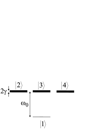
Figure 1: Level scheme of a $J_{g}=0\rightarrow J_{e}=1$ dipole transition, with atomic transition frequency $\omega_{0}$, and natural linewidth $2\gamma$. The sublevels $\left|1\right\rangle$ and $\left|3\right\rangle$ have magnetic quantum number $m=0$. Sublevels $\left|2\right\rangle$ and $\left|4\right\rangle$ correspond to $m=-1$ and $m=1$, respectively.

and

$$\mathbf{\hat{e}}_{\pm 1}=\mp\frac{1}{\sqrt{2}}(\mathbf{\hat{e}}_{x}\pm i\mathbf{\hat{e}}_{y}),\quad\mathbf{\hat{e}}_{0}=\mathbf{\hat{e}}_{z}$$ (8)

are the unit vectors of the spherical basis. In the free field Hamiltonian, $a^{(\dagger)}_{{\bf k},s}$ annihilates (creates) a photon in the reservoir mode with wavevector k and transverse polarization $\boldsymbol{\varepsilon}_{\textbf{k},s}$, where $s$ is the polarization index.

The interaction Hamiltonians $H_{\rm AF}$ and $H_{\rm AL}$ are written in rotating wave and dipole approximation. The coupling constant between atom $\alpha$, located at point $\textbf{r}_{\alpha}$, and the vacuum mode $(\textbf{k},s)$ reads

$$\kappa_{\bf k}({\bf r}_{\alpha})=-id\left(\frac{\omega_{k}}{2\hbar\epsilon_{0}V}\right)^{1/2}e^{i\textbf{k}\cdot{\bf r}_{\alpha}}\,,$$ (9)

where $d$ is a reduced matrix element, $\epsilon_{0}$ is the permittivity of the vacuum, and $V$ is the quantization volume. The coupling of atom $\alpha$ to the laser field

$${\bf E}_{L}({\bf r})=\boldsymbol{\varepsilon}_{L}{\cal E}e^{i(\textbf{k}_{L}\cdot{\bf r}-\omega_{L}t)}+{\rm c.c.}$$ (10)

is characterized by a position-dependent Rabi frequency

$$\Omega_{\alpha}=\frac{2d{\cal E}}{\hbar}e^{i\textbf{k}_{L}\cdot{\bf r}_{\alpha}}\equiv\Omega e^{i\textbf{k}_{L}\cdot{\bf r}_{\alpha}}\,.$$ (11)

The figure of merit in our present study is the average value of the stationary intensity $I({\bf r})$ with polarization $\boldsymbol{\varepsilon}$, scattered in a direction close to backscattering $-\textbf{k}_{L}$:

$$I(\textbf{r})=\lim_{t\to\infty}\langle[\boldsymbol{\varepsilon}\cdot{\bf E}^{(-)}({\bf r},t)][\boldsymbol{\varepsilon}^{*}\cdot{\bf E}^{(+)}({\bf r},t)]\rangle\,.$$ (12)

${\bf E}^{(-/+)}({\bf r},t)$ is the negative/positive frequency component of the source field operators, given by the superposition of the retarded fields radiated by all atomic dipoles, that is projected onto the polarization vector $\boldsymbol{\varepsilon}$, upon detection,

$$\boldsymbol{\varepsilon}^{*}\cdot{\bf E}^{(+)}({\bf r},t)=\frac{\omega_{0}^{2}}{4\pi\varepsilon_{0}c^{2}r}\sum_{\alpha=1}^{N}\boldsymbol{\varepsilon}^{*}\cdot\textbf{D}_{\alpha}(t_{\alpha})e^{-i\textbf{k}\cdot{\bf r}_{\alpha}}\,,$$ (13)

with $t_{\alpha}=t-|{\bf r}-{\bf r}_{\alpha}|/c$, and k the wave vector with the wave length of the injected laser radiation, pointing in the observation direction (note that all the nontrivial spectral information is contained in the time dependence of the atomic dipole correlation function). This expression follows immediately from generalizing familiar expressions for the far field radiated by a single atom Carmichael to the present case of an atomic cloud, with the cloud’s diameter much smaller than the distance to the detector.

The total scattered intensity is then obtained by inserting (13) and its conjugate into (12), and reads, up to a prefactor,

$$I=\sum_{\alpha,\beta=1}^{N}{\langle[\boldsymbol{\varepsilon}\cdot\textbf{D}^{\dagger}_{\alpha}][\boldsymbol{\varepsilon}^{*}\cdot\textbf{D}_{\beta}]\rangle}_{\text{ss}}e^{i\textbf{k}\cdot{\bf r}_{\alpha\beta}}\,,$$ (14)

where ‘ss’ stands for steady state, and ${\bf r}_{\alpha\beta}\equiv{\bf r}_{\alpha}-{\bf r}_{\beta}$.

II.2 Coherent backscattering and polarization channels

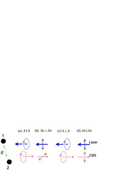
Figure 2: (Color online) Elementary configuration for the polarization-selective detection of the coherent backscattering signal (CBS) (dashed arrows) from laser light (thick arrows) scattering on two atoms 1 and 2 (black circles). The dipole-dipole coupling strength between the atoms is given by the coupling constant $g$. Backscattered photons are detected in four polarization channels: (a) right circular in, left circular out (with respect to a fixed observation direction; $h\parallel h$); (b) linear in, orthogonal linear out ($lin\perp lin$); (c) right circular in, right circular out ($h\perp h$); (d) linear in, parallel linear out ($lin\parallel lin$). Note that in cases (c) and (d) CBS appears on the background of single scattering from independent atoms.

The structure of Eq. (14), together with (7), shows that all three transitions between each atom’s electronic levels (see Fig. 1) will in general contribute to the scattered light intensity – the relative weights of their contributions depend on the observation direction and on the detected polarization channel.

The unit polarization vector $\boldsymbol{\varepsilon}$ may be chosen either in a circular or in a linear basis. For circular polarization, it is convenient to use the so-called helicity basis, in which the quantization axis is directed along the probe direction $\textbf{k}_{L}$. In the case of linear polarization, the quantization axis is conveniently chosen along the incident polarization vector $\mathbf{\hat{e}}_{0}$ (perpendicular to $\textbf{k}_{L}$). For both choices, $\boldsymbol{\varepsilon}$ has, in general, three nonzero projections on the unit vectors of the spherical basis, at finite angles between ${\bf k}$ and $-\textbf{k}_{L}$.

From now on, we will use an approximation which is legitimate at small scattering angles (k is very close to $-\textbf{k}_{L}$), a common situation in CBS experiments. One is interested in signals at very small angles $\theta\simeq 1/k\ell$ around the backscattering direction (the mean free path $\ell$ is the average distance between consecutive scatterers, and $k\ell\gg 1$ in dilute atomic gases). Since the geometric change of $\boldsymbol{\varepsilon}$ varies only with the cosine of the scattering angle $\theta\ll 1$, we can take $\boldsymbol{\varepsilon}$ constant, equal to its value at exact backscattering.

With these conventions, Eq. (14) can be specialized for the four polarization channels traditionally selected in CBS experiments (see Fig. 2).

II.2.1 Helicity preserving channel $(h\parallel h)$

In the helicity preserving channel, the incident radiation is circularly polarized, and drives either the $\left|1\right\rangle\rightarrow\left|2\right\rangle$ or the $\left|1\right\rangle\rightarrow\left|4\right\rangle$ transition. The backscattered light is then observed in the orthogonal polarization channel (with the same helicity, since the propagation direction is reversed) and must be radiated by the $\left|1\right\rangle\rightarrow\left|4\right\rangle$ or the $\left|1\right\rangle\rightarrow\left|2\right\rangle$ transition, respectively. Both combinations are completely equivalent, and for the case $\boldsymbol{\varepsilon}_{L}=\mathbf{\hat{e}}_{+1}$, $\boldsymbol{\varepsilon}=\mathbf{\hat{e}}_{-1}$, the total backscattered intensity reads

$$I=\sum_{\alpha}\langle\sigma_{22}^{\alpha}\rangle_{\rm ss}+\sum_{\alpha\neq\beta}\langle\sigma_{21}^{\alpha}\sigma_{12}^{\beta}\rangle_{\rm ss}e^{i\textbf{k}\cdot{\bf r}_{\alpha\beta}}.$$ (15)

II.2.2 $lin\perp lin$ channel

In the $lin\perp lin$ channel, $\boldsymbol{\varepsilon}_{L}=\mathbf{\hat{e}}_{0}$. We further assume, without loss of generality, that the laser field is propagating along the $x$-axis, such that the detected photons are polarized along the $y$-axis. In the spherical basis, $\boldsymbol{\varepsilon}=\mathbf{\hat{e}}_{y}=i(\mathbf{\hat{e}}_{-1}+\mathbf{\hat{e}}_{+1})/\sqrt{2}$, leading to the expression

$$I = \sum_{\alpha}\bigl{(}\langle\sigma_{22}^{\alpha}\rangle_{\rm ss}+\langle\sigma_{44}^{\alpha}\rangle_{\rm ss}+\langle\sigma_{24}^{\alpha}\rangle_{\rm ss}+\langle\sigma_{42}^{\alpha}\rangle_{\rm ss}\bigr{)}$$

$$+\sum_{\alpha\neq\beta}e^{i\textbf{k}\cdot{\bf r}_{\alpha\beta}}\bigr{(}\langle\sigma_{41}^{\alpha}\sigma_{14}^{\beta}\rangle_{\rm ss}+\langle\sigma_{21}^{\alpha}\sigma_{12}^{\beta}\rangle_{\rm ss}\bigr{.}$$

. $$+\langle\sigma_{41}^{\alpha}\sigma_{12}^{\beta}\rangle_{\rm ss}+\langle\sigma_{21}^{\alpha}\sigma_{14}^{\beta}\rangle_{\rm ss}\bigr{)}.$$ (16)

II.2.3 Flipped helicity channel $(h\perp h)$

With incident polarization $\boldsymbol{\varepsilon}_{L}=\mathbf{\hat{e}}_{+1}$ as before, the $h\perp h$ channel corresponds to $\boldsymbol{\varepsilon}=\mathbf{\hat{e}}_{+1}$, such that

$$I=\sum_{\alpha}\langle\sigma_{44}^{\alpha}\rangle_{\rm ss}+\sum_{\alpha\neq\beta}\langle\sigma_{41}^{\alpha}\sigma_{14}^{\beta}\rangle_{\rm ss}e^{i\textbf{k}\cdot{\bf r}_{\alpha\beta}}\,.$$ (17)

II.2.4 $lin\parallel lin$ channel

Finally, in the $lin\parallel lin$ channel, the incoming and outgoing photons are linearly polarized along the same axis, $\boldsymbol{\varepsilon}_{L}=\boldsymbol{\varepsilon}=\mathbf{\hat{e}}_{0}$, and we obtain

$$I=\sum_{\alpha}\langle\sigma_{33}^{\alpha}\rangle_{\rm ss}+\sum_{\alpha\neq\beta}\langle\sigma_{31}^{\alpha}\sigma_{13}^{\beta}\rangle_{\rm ss}e^{i\textbf{k}\cdot{\bf r}_{\alpha\beta}}\,.$$ (18)

The above expressions systematically decompose into two parts: Single atom, steady state dipole expectation values express the intensities radiated by individual atoms, while correlation functions of distinct atomic dipoles, multiplied by phases which depend on the relative position of the atoms, account for the interference contribution.

We now show how to evaluate these different steady state expectation values explicitly, before performing the ensemble average over the atomic positions, in Sec. III.

II.3 Equations of motion for the atomic correlation functions

The dynamics of the atomic dipole operators’ expectation values as well as of the dipole-dipole correlators which enter (15-18) is governed by the master equation lehmberg

$$\langle\dot{Q}\rangle=\sum_{\alpha=1}^{N}\langle{\cal L}_{\alpha}Q\rangle+\sum_{\alpha\neq\beta=1}^{N}\langle{\cal L}_{\alpha\beta}Q\rangle,$$ (19)

where the Liouvillians ${\cal L}_{\alpha}$ and ${\cal L}_{\alpha\beta}$ generate the time evolution of an arbitrary atomic operator $Q$, for independent and interacting atoms, respectively, and $\langle\ldots\rangle={\rm Tr}\,(\ldots\rho(0))$, with $\rho(0)$ being the initial density operator of the $N$-atoms-field system, indicates the quantum mechanical expectation value.

In the co-rotating frame with respect to the driving field at frequency $\omega_{L}$, and after the standard electric dipole, rotating wave, and Born-Markov approximations, ${\cal L}_{\alpha}$ and ${\cal L}_{\alpha\beta}$ read lehmberg :

$${\cal L}_{\alpha}Q = -i\delta[\textbf{D}^{\dagger}_{\alpha}\cdot\textbf{D}_{\alpha},Q]-\frac{i}{2}[\Omega_{\alpha}(\textbf{D}^{\dagger}_{\alpha}\cdot\boldsymbol{\varepsilon}_{L})+\Omega^{*}_{\alpha}(\textbf{D}_{\alpha}\cdot\boldsymbol{\varepsilon}_{L}^{*}),Q]+\gamma\left(\textbf{D}^{\dagger}_{\alpha}\cdot[Q,\textbf{D}_{\alpha}]+[\textbf{D}^{\dagger}_{\alpha},Q]\cdot\textbf{D}_{\alpha}\right),$$ (20)

$${\cal L}_{\alpha\beta}Q = \textbf{D}^{\dagger}_{\alpha}\cdot\overleftrightarrow{\bf T}(g,{\bf\hat{n}})\cdot[Q,\textbf{D}_{\beta}]+[\textbf{D}^{\dagger}_{\beta},Q]\cdot\overleftrightarrow{\bf T}^{*}(g,{\bf\hat{n}})\cdot\textbf{D}_{\alpha}\,,$$ (21)

where the radiative dipole-dipole interaction due to exchange of photons between the atoms is described by the tensor $\overleftrightarrow{\bf T}(g,{\bf\hat{n}})=\gamma g\overleftrightarrow{\boldsymbol{\Delta}}$. This interaction has a certain strength depending on the distance between the atoms, via

$$g=\frac{3i}{2k_{0}r_{\alpha\beta}}e^{ik_{0}r_{\alpha\beta}},$$ (22)

with $k_{0}=\omega_{0}/c$, and on the life time of the excited atomic levels, through $\gamma$.

The coupling constant $|g|\ll 1$ is small in the far-field ($k_{0}r_{\alpha\beta}\gg 1$), where near-field interaction terms of order $(k_{0}r_{\alpha\beta})^{-2}$ and $(k_{0}r_{\alpha\beta})^{-3}$ can be neglected (which, at higher atomic densities, could also be retained in our formalism). The projector $\overleftrightarrow{\boldsymbol{\Delta}}=\overleftrightarrow{\openone}-{\bf\hat{n}\hat{n}}$ on the transverse plane defined by the unit vector $\bf\hat{n}$ along the connecting line between the atoms $\alpha$ and $\beta$ is explicitly given through

$$\overleftrightarrow{\openone} = -\mathbf{\hat{e}}_{-1}\mathbf{\hat{e}}_{+1}+\mathbf{\hat{e}}_{0}\mathbf{\hat{e}}_{0}-\mathbf{\hat{e}}_{+1}\mathbf{\hat{e}}_{-1},$$ (23a)

$${\bf\hat{n}} = \frac{e^{i\phi}\sin\vartheta}{\sqrt{2}}\mathbf{\hat{e}}_{-1}+\cos\vartheta\mathbf{\hat{e}}_{0}-\frac{e^{-i\phi}\sin\vartheta}{\sqrt{2}}\mathbf{\hat{e}}_{+1}\,.$$ (23b)

The angles $(\vartheta,\phi)$, which fix the direction of the connecting vector between two atoms (with respect to the backscattering direction), will have to be averaged over further down note .

It should be kept in mind here that the master equation treatment implies a trace over the modes of the free field, and that the Markov approximation implies some coarse graining on the time axis. Thus, $\gamma$ and $g$ are the only remnants of the coupling to the electromagnetic vacuum, giving rise to some effective dynamics of the atomic operators, on time scales which are long with respect to the time scales of single absorption and emission events from and into the electromagnetic reservoir. Only by expansion of the solutions of (20,21) in powers of $g$ will we be able to distinguish multiple scattering contributions of increasing order, since, formally, all elastic and inelastic processes are lumped together in (20,21) by $\Omega$, $\gamma$, and $g$. This renders the master equation treatment somewhat less transparent or at least less intuitive as compared to the scattering theoretical approach wellens04 , but bears the qualitative improvement of yielding results which are valid for arbitrary saturation parameter $s$.

Note that the Markovian master equation (19) ignores retardation effects due to a finite photon propagation time between scatters. This approximation is justified when $\max(r_{\alpha\beta})\propto\ell\ll c/\gamma$ lehmberg . In typical experiments with sharply defined, resonant optical dipole transitions labeyrie03 , both the condition of diluteness, $k\ell\gg 1$, and of ‘instantaneous’ propagation are very well satisfied.

The equation (19) leads to a system of linear, coupled differential equations with constant coefficients for the atomic correlation functions. The algebra of the $N$-atoms operators is spanned by tensor products of individual operators $\sigma^{\alpha}_{kl}=\left|k\right\rangle_{\alpha}\left\langle l\right|_{\alpha}$, each acting on the $N$-fold tensor product of the four dimensional Hilbert space in which the internal states of a single atom are represented. For the free evolution of a single atom ($N=1$), $Q_{\alpha}$ can be chosen in a complete orthonormal set of 16 basis operators (see also Sect. II.4 below, for details).

For our treatment of CBS, we need to include at least two-atoms operators in (19). For $N=2$, the number of equations in (19) is $255=16^{2}-1$ (there is one constant of motion). In matrix notation, the resulting equation of motion reads

$$\dot{\langle{\bf Q}\rangle}=({\bf A}~{}+~{}{\bf V}){\langle{\bf Q}\rangle}+{\bf j}\,,$$ (24)

where the elements of the vector $\langle{\bf Q}\rangle$ are given by the expectation values of the complete orthonormal set of two-atom operators. The elements $A_{nm}$, $V_{nm}$ and $j_{n}$ of the matrices ${\bf A}$, ${\bf V}$, and of the vector ${\bf j}$, are derived from the equation for the element $\langle Q_{n}\rangle$ in (24):

$$\langle({\cal L}_{\alpha}~{}+~{}{\cal L}_{\beta})Q_{n}\rangle = \sum_{m=1}^{255}A_{nm}\langle Q_{m}\rangle+j_{n},$$ (25)

$$\langle({\cal L}_{\alpha\beta}~{}+~{}{\cal L}_{\beta\alpha})Q_{n}\rangle = \sum_{m=1}^{255}V_{nm}\langle Q_{m}\rangle.$$ (26)

From the decomposition of (24) into (25) and (26) it is apparent that the matrix ${\bf A}$ generates the evolution of uncoupled atoms, whereas ${\bf V}$ describes their interaction via the exchange of photons.

II.4 Green’s matrix and matrix ${\bf A}$

In order to solve (24), we first need its represention in a suitable operator basis. Thereafter, we will derive a solution for independent atoms (that is, we will ignore the matrix ${\bf V}$, which mediates the interatomic correlations) by a Laplace transform. The thus established relation between the Green’s matrix for the non-interacting two-atom system and the matrix ${\bf A}$ will then serve as a basis for a systematic, perturbative treatment of the interacting case, at increasing order in the coupling constant $g$.

Let us first consider the dynamics of a single four-level system. An expectation value of a single-atom operator $Q_{\alpha}$ obeys the equation of motion

$$\langle\dot{Q_{\alpha}}\rangle=\langle{\cal L}_{\alpha}Q_{\alpha}\rangle,$$ (27)

where the superoperator ${\cal L}_{\alpha}$ is given by eq. (20). The master equation (27) describes resonance fluorescence of the laser-driven $J_{g}=0\rightarrow J_{e}=1$ atomic dipole transition. $Q_{\alpha}$ belongs to the complete orthonormal set $S^{\alpha}$ of 16 operators for the four-level system,

$$Q_{\alpha}\in S^{\alpha}=\Bigl{\{}\frac{\openone^{\alpha}}{2},\frac{\mu_{1}^{\alpha}}{2},\frac{\mu_{2}^{\alpha}}{2},\frac{\mu_{3}^{\alpha}}{2},\underbrace{\sigma^{\alpha}_{kl}\;(k\neq l=1\ldots 4)}_{12\,{\rm operators}}\Bigr{\}}\,,$$ (28)

where

$$= \sigma_{11}+\sigma_{22}+\sigma_{33}+\sigma_{44}\,,$$ (29a)

$$\mu_{1} = \sigma_{22}-\sigma_{33}+\sigma_{44}-\sigma_{11}\,,$$ (29b)

$$\mu_{2} = \sigma_{22}-\sigma_{33}-\sigma_{44}+\sigma_{11}\,,$$ (29c)

$$\mu_{3} = \sigma_{22}+\sigma_{33}-\sigma_{44}-\sigma_{11}\,.$$ (29d)

It is easy to check that for the elements of $S^{\alpha}$ the orthonormality condition ${\rm Tr}\,[Q_{n}Q_{m}^{T}]=\delta_{nm}$ holds. In this representation, equation (27) turns into a linear matrix equation for the vector $\langle{\bf Q}_{\alpha}(t)\rangle$, whose 16 elements are the quantum mechanical expectation values of the elements of $S^{\alpha}$. Since the atomic levels’ dynamics are uncoupled, except for the laser-driven transition, it can be solved analytically. The dynamics of the driven transition is equivalent to the one of a two-level system.

For two atoms, $Q^{\alpha\beta}\in S^{\alpha}\otimes S^{\beta}$, and the vector of the two-atoms correlation functions,

$$\langle{\bf Q}^{\alpha\beta}(t)\rangle=[\langle\openone^{\alpha}\otimes\openone^{\beta}\rangle/4,\ldots,\langle\sigma^{\alpha}_{kl}\otimes\sigma_{kl}^{\beta}\rangle]^{T}\,,$$ (30)

consists of 256 elements. The evolution operator of uncoupled atoms reads

$$e^{{\cal L}_{0}t}=e^{{\cal L}_{\alpha}t}\otimes e^{{\cal L}_{\beta}t}.$$ (31)

A Laplace transform $\int_{0}^{\infty}dte^{-zt}e^{{\cal L}_{0}t}$ of (31) gives the Green’s function (or resolvent) $G_{\alpha\beta}(z)=(z-{\cal L}_{0})^{-1}$ of the Liouvillian ${\cal L}_{0}={\cal L}_{\alpha}+{\cal L}_{\beta}$. In the two-atom basis $S^{\alpha}\otimes S^{\beta}$, $G_{\alpha\beta}(z)$ has a matrix representation ${\bf G}_{\alpha\beta}(z)$. This matrix has the following block structure:

$${\bf G}_{\alpha\beta}(z)=\begin{pmatrix}z^{-1}&\vdots&{\bf 0}^{T}\\ {3}\\ z^{-1}{\bf j}&\vdots&{\bf G}_{0}(z)\end{pmatrix},$$ (32)

where vectors ${\bf 0}$ (zero vector) and ${\bf j}$ have $255$ elements, and ${\bf G}_{0}(z)$ is the truncated ($255\times 255$) Green’s matrix. As seen from (32), the first column of matrix ${\bf G}_{\alpha\beta}(z)$ has a pole at $z=0$. This pole appears because the first element of the vector $\langle{\bf Q}^{\alpha\beta}(t)\rangle$, $\langle\openone^{\alpha}\otimes\openone^{\beta}\rangle\equiv{\rm Tr}\,\rho_{0}$, is a constant of motion. All other elements of the vector $\langle{\bf Q}^{\alpha\beta}(t)\rangle$ are time-dependent. The steady-state solution of the truncated vector, $\langle{\bf Q}(t)\rangle$, which is obtained from $\langle{\bf Q}^{\alpha\beta}(t)\rangle$ after exclusion of its first element, ${\rm Tr}\,\rho_{0}$, is defined as $\langle{\bf Q}\rangle_{\rm ss}=\lim_{z\to 0}z\langle\tilde{{\bf Q}}(z)\rangle$, where $\langle\tilde{{\bf Q}}(z)\rangle$ is the Laplacian image of the vector $\langle{\bf Q}(t)\rangle$. This limit is evaluated to give

$$\langle{\bf Q}\rangle_{\rm ss}={\bf G}_{0}{\bf j},$$ (33)

where ${\bf G}_{0}\equiv{\bf G}_{0}(0)$. Comparison of (33) with the steady-state solution of Eq. (25), $\langle{\bf Q}\rangle_{\rm ss}=-{\bf A}^{-1}{\bf j}$, now shows that ${\bf G}_{0}\equiv-{\bf A}^{-1}$.

II.5 Perturbative restriction to low scattering orders

The theoretical description of coherent backscattering is relatively simple in two opposite regimes: either in the diffusive regime of fully developed multiple scattering in optically thick media, where long paths or high scattering orders yield the celebrated conical line-shape of the CBS signal, or, on the contrary, in the regime of scattering by optically thin media (or in the presence of suppression of interference), where only double scattering needs to be considered jonckheere00 ; bidel02 . Indeed, it is in the double-scattering regime where the first experimental observation of a CBS reduction due to the non-linear saturation of atomic dipole transitions was reported chaneliere03 . We limit our present analytical and numerical analysis to this specific case.

In our master equation framework, all information on multiple scattering processes is contained in the correlation functions of dipole-dipole interacting atoms. The double scattering contribution to the scattered light intensity from a given pair of atoms, resulting from the exchange of two photons between the atoms, is obtained by perturbative expansion of the respective correlation functions to second order in the dipole-dipole coupling constant $|g|$. This contribution depends only on the observables related to the two selected atoms, and not on those of the rest of the atoms in the cloud, since corrections to the mean intensity due to the latter would be of higher order in $|g|$ ($|g|^{3}$, etc.). Therefore, to find the double scattering contribution, we will solve the master equation (19) for two fixed atoms $\alpha=1,2$. Subsequently, we have to add up all double scattering contributions resulting from the atoms located at random positions. In other words, we need to perform appropriate disorder averages of the solution for two fixed atoms.

This setup defines the simplest possible model describing CBS. Indeed, double scattering is the lowest order process which gives rise to distinct scattering amplitudes that can interfere constructively. Despite its simplicity, this model allows for a qualitative assessment of the impact of nonlinear scattering processes on the CBS signal, whereas propagation effects in the bulk of the scattering medium are beyond its reach. It also needs to be considered that nonlinear scattering processes are induced by high laser intensities, at which atoms are rapidly accelerated out of resonance. Within our model, we neglect this acceleration, by focusing exclusively on the coupling of photons to the internal atomic degrees of freedom. Such an approximation is justified, since the mechanical action of light on atoms can be experimentally compensated by shortening the CBS probe duration, as realized, e.g., in chaneliere03 .

For our perturbative solution of Eq. (24), we take advantage of the small parameter $g$ in (21) (defined in Eq. (22)), and expand in a power series of ${\bf V}$. The $n$th order

$$\langle{\bf Q}\rangle^{[n]}_{\rm ss}=({\bf G}_{0}{\bf V})^{n}{\bf G}_{0}{\bf j}$$ (34)

of the stationary solution of Eq. (24) gives the two-atoms correlation functions resulting from $n$ exchanged photons, and generally includes also recurrent scattering (a photon visits the same atom several times). We recall that, in the regime of elastic scattering from dilute samples of resonant scatterers, higher scattering orders can be accounted for by considering more scatterers, while recurrent scattering is irrelevant tiggelen96 . In contrast, as one proceeds to the strong scattering regime, with denser clouds of resonant scatterers, the effect of recurrent scattering manifests by a gradual reduction of the enhancement factor as compared to its maximum value $2.0$ wiersma95 . We will see in Sect. IV.3.1 below that Eq. (34) generally including recurrent scattering contributions is fully compatible with neglecting these in the linear regime.

Total intensities for the double scattering contribution are given by the third term (proportional to $|g|^{2}$) of the above expansion of the correlation functions which enter Eqs. (15-18), with the general structure

$$\langle{\bf Q}\rangle^{[2]}_{\rm ss}={\bf G}_{0}{\bf V}{\bf G}_{0}{\bf V}{\bf G}_{0}{\bf j}.$$ (35)

Note that the matrix ${\bf V}$ depends on $\overleftrightarrow{\bf\Delta}$, though neither on $\boldsymbol{\varepsilon}_{L}$ nor on $\boldsymbol{\varepsilon}$. Indeed, information about the laser polarization is carried by the Liouvillian (20), which governs the evolution of independent atoms. As for $\boldsymbol{\varepsilon}$, it does not appear in the equations of motion for the atomic correlation functions at all – but it defines which elements of the vector $\langle{\bf Q}\rangle^{[2]}_{\rm ss}$ contribute to the observed signal, as evident from Eq. (14).

II.6 Elastic component of double scattering

The total backscattered intensity (14) has a spectral distribution that contains an elastic and, beyond the weak field limit, also an inelastic component. The detected intensity is the correlation function of the source field amplitudes radiated by the atomic dipoles.

Its elastic component stems from the classically radiating dipoles, i.e., from the nonfluctuating factorized averages $\langle\sigma_{i\neq j}^{\alpha}\rangle$ cohen_tannoudji . Hence, the elastic intensity is given by the product of the expectation values of the atomic dipoles,

$$I^{\rm el}=\sum_{\alpha,\beta=1}^{N}{\langle\boldsymbol{\varepsilon}\cdot\textbf{D}^{\dagger}_{\alpha}\rangle}_{\text{ss}}{\langle\boldsymbol{\varepsilon}^{*}\cdot\textbf{D}_{\beta}\rangle}_{\text{ss}}e^{i\textbf{k}\cdot{\bf r}_{\alpha\beta}}\,.$$ (36)

In the helicity preserving channel $h\parallel h$, this reads

$$I^{\rm el}=\sum_{\alpha}|\langle\sigma_{21}^{\alpha}\rangle_{\rm ss}|^{2}+\sum_{\alpha\neq\beta}\langle\sigma_{21}^{\alpha}\rangle_{\rm ss}\langle\sigma_{12}^{\beta}\rangle_{\rm ss}e^{i\textbf{k}\cdot{\bf r}_{\alpha\beta}}.$$ (37)

Analogous expessions for the elastic component can be derived from Eqs. (16-18) in the other channels.

The double scattering contribution $I^{\rm el}_{2}$ to the elastic intensity, which we are interested in, and which is proportional to $|g|^{2}$, is obtained from the corresponding power series expansion, Eqs. (34,35), of the individual factors entering the above expression, in the coupling constant. In this expansion, there emerge symmetric and asymmetric combinations, like $\langle\sigma_{21}^{1}\rangle_{\rm ss}^{[1]}\langle\sigma_{12}^{2}\rangle_{\rm ss}^{[1]}$, and $\langle\sigma_{21}^{1}\rangle_{\rm ss}^{[2]}\langle\sigma_{12}^{2}\rangle_{\rm ss}^{[0]}$, respectively. To ease the physical interpretation of these various terms, remember that, by virtue of (34), the superscripts ‘$[0]$’, ‘$[1]$’, and ‘$[2]$’ signal the scattering of a photon from one single atom $\alpha$ (‘$[0]$’), subsequently from atom $\alpha$ and then from atom $\beta$ (‘$[1]$’), and the rescattering of the same photon from atom $\alpha$, after a first encounter with $\alpha$ and subsequent scattering from $\beta$ (‘$[2]$’).

In the $h\parallel h$ and $lin\perp lin$ channel, only symmetric combinations contribute to the elastic component of the CBS intensity, since the lowest order expectation value of a single atom’s coherence in the analyzed transition (like $\langle\sigma_{12}^{2}\rangle_{\rm ss}^{[0]}$ in the helicity preserving channel) must vanish: at lowest order, the atom is not coupled to the other atom, nor is the transition directly driven by the injected laser. By the same argument, also the single scattering intensities from non-interacting atoms (arising from the first sum on the right hand side of Eq. (37)) are projected out, and an interference signal from purely multiple scattering sequences is measured in these channels (unless the atoms have a degenerate ground state and can undergo transitions between different Zeeman-sublevels mueller01 ).

In the $h\perp h$ and $lin\parallel lin$ channels, both, symmetric and asymmetric combinations of products of the dipole averages contribute.

Altogether, at second order in the coupling constant, the elastic backscattering intensity from two fixed atoms is obtained from the evaluation of the zeroth-, first-, and second-order stationary solutions $\langle{\bf Q}\rangle^{[0]}_{\rm ss}$, $\langle{\bf Q}\rangle^{[1]}_{\rm ss}$, and $\langle{\bf Q}\rangle^{[2]}_{\rm ss}$ of Eq. (24). The backscattering intensity from a cloud of randomly located atoms is finally derived through an appropriate disorder average.

III Disorder averaging

Coherent backscattering is such a surprising effect because it survives the ensemble average over random positions of the scatterers, which destroys all other speckle-like interferences. The precise procedure of disorder averaging is important as soon as one is interested in the exact shape and angular width of the CBS cone. Here, we rather focus on the impact of the atomic saturation on the maximum CBS intensity, in the exact backscattering direction. Since saturation effects are independent of the precise averaging prescription, we choose a procedure as simple as possible: an (i) isotropic average of the relative orientation ${\bf\hat{n}}$ of the atoms over the unit sphere is followed by (ii) an average of the inter-atomic distance $r_{12}$ over an interval of the order of the laser wavelength, around their typical distance $\ell$:

$$\langle\ldots\rangle_{\rm conf}=\frac{k_{L}}{4\pi}\int_{\ell-2\pi/k_{L}}^{\ell+2\pi/k_{L}}dr_{12}\int d\Omega_{\bf\hat{n}}\ldots.$$ (38)

After the evaluation of (38), the final expression for the backscattering intensity has a general structure which decomposes into ‘ladder’ and ‘crossed’ contributions, respectively. The ladder terms collect the intensities scattered by individual atomic dipoles (in a diagrammatic representation, they arise from the summation of co-propagating amplitudes Sheng along a sequence of scatterers), in an incoherent sum, whereas the crossed terms stem from the interference of amplitudes radiated by distinct dipoles (counter-propagating amplitudes in a diagrammatic picture), and are garnished by the associated phases. Through this phase factor, the interference part depends on the angle $\theta$ between the wavevector k of the final photon and the backscattering direction $-\textbf{k}_{L}$. As an example, the ladder and crossed terms in the $h\parallel h$ channel read, by virtue of Eq. (15),

$$L^{\rm tot}_{2} = \langle\langle\sigma_{22}^{1}\rangle^{[2]}_{\rm ss}+\langle\sigma_{22}^{2}\rangle^{[2]}\rangle_{\rm ss}\rangle_{\rm conf},$$ (39)

$$C^{\rm tot}_{2}(\theta) = 2\,{\rm Re}\,\langle\langle\sigma^{1}_{21}\sigma^{2}_{12}\rangle^{[2]}_{\rm ss}e^{i\textbf{k}\cdot{\bf r}_{12}}\rangle_{\rm conf}\,,$$ (40)

respectively.

The enhancement factor $\alpha$, which is the figure of merit for the quantification of CBS, is given by

$$\alpha=1+\frac{C^{\rm tot}_{2}(0)}{L^{\rm tot}_{2}}\,.$$ (41)

An analogous expression for the elastic CBS component follows from Eq. (37), with ladder and crossed terms $L^{\rm el}_{2}$ and $C^{\rm el}_{2}(\theta)$.

IV Results

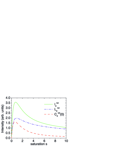
Figure 3: (Color online) Saturation dependence of the total double scattering contribution $I_{2}^{\rm tot}$ to the CBS signal in the $h\parallel h$ channel, decomposed in its ladder and interference parts $L_{2}^{\rm tot}$ and $C_{2}^{\rm tot}$, according to Eqs. (46,47), at exact resonance $\delta=0$. At finite saturation $s$, the interference term $C_{2}^{\rm tot}$ drops below the ladder contribution $L_{2}^{\rm tot}$, indicating a loss of coherence. At large $s\geq 1$, the total double scattering intensity must decrease with $s$, since the scattering cross section of the emitting atom drops as $s^{-1}$.

We now proceed to evaluate the general expressions derived above, for the four typical polarization channels analyzed in the laboratory: $h\parallel h$, $lin\perp lin$, $h\perp h$, and $lin\parallel lin$. Analytical results for vanishing detuning $\delta$ will be complemented by some numerical results for $\delta\neq 0$.

IV.1 $h\parallel h$ channel

IV.1.1 Total intensity, at zero detuning

In Eqs. (15) and (37) we assumed that the $\left|1\right\rangle\rightarrow\left|4\right\rangle$ transition is laser-driven. Photons with preserved helicity originate from the $\left|2\right\rangle\rightarrow\left|1\right\rangle$ transitions, and $\boldsymbol{\varepsilon}_{L}=\mathbf{\hat{e}}_{+1}$, $\boldsymbol{\varepsilon}=\mathbf{\hat{e}}_{-1}$. The total double scattering intensity for two fixed atoms reads, by virtue of Eqs. (15) and (35), at second order in $g$ and vanishing detuning $\delta=0$:

$$2\,{\rm Re}\,\{\langle\sigma_{21}^{1}\sigma_{12}^{2}\rangle_{\rm ss}^{[2]}e^{i{\bf k}\cdot{\bf r}_{12}}\} = |g|^{2}|\overleftrightarrow{\boldsymbol{\Delta}}_{+1,+1}|^{2}\frac{R_{1}(s)}{(4+s)P(s)}$$ (42)

$$\times\cos\{({\bf k}+{\bf k}_{L})\cdot{\bf r}_{12}\},$$

$$\langle\sigma_{22}^{1}\rangle_{\rm ss}^{[2]}+\langle\sigma_{22}^{2}\rangle_{\rm ss}^{[2]} = |g|^{2}|\overleftrightarrow{\boldsymbol{\Delta}}_{+1,+1}|^{2}\frac{R_{2}(s)}{P(s)}\,.$$ (43)

$R_{1}(s)$, $R_{2}(s)$, and $P(s)$ are polynomial expressions in the saturation parameter $s$,

$$R_{1}(s) = \frac{2}{9}\left(6912s+3168s^{2}\right.$$ (44a)

$$\left.+264s^{3}+20s^{4}+s^{5}\right),$$

$$R_{2}(s) = \frac{1}{3}\left(1152s+528s^{2}+132s^{3}+7s^{4}\right),$$ (44b)

$$P(s) = (1+s)^{2}(12+s)(32+20s+s^{2}),$$ (44c)

and

$$\overleftrightarrow{\boldsymbol{\Delta}}_{q,q^{\prime}}\equiv\mathbf{\hat{e}}_{q}\cdot\overleftrightarrow{\boldsymbol{\Delta}}\cdot\mathbf{\hat{e}}_{q^{\prime}},\quad(q,q^{\prime}=\pm 1,0)\,.$$ (45)

The configuration average over (43) and (42), defined in Eq. (38), leads to the final result

$$C^{\rm tot}_{2}(\theta) \simeq \frac{|\tilde{g}|^{2}R_{1}(s)}{(4+s)P(s)}\Bigl{(}\frac{2}{15}-\frac{(k\ell\theta)^{2}}{35}\Bigr{)},$$ (46)

$$L^{\rm tot}_{2} = \frac{2|\tilde{g}|^{2}R_{2}(s)}{15P(s)},$$ (47)

with $\tilde{g}=g|_{r_{\alpha\beta}=\ell}$ (see Eq. (22)). The scattering angle $\theta=2\arcsin\{|{\bf k}+{\bf k}_{L}|/2k_{L}\}\ll 1$ with respect to the backscattering direction was assumed to be sufficiently small herein. A power series expansion of Eqs. (46,47) to second order in $s$ reproduces the diagramatically obtained result of wellens04 ,

$$C^{\rm tot}_{2}\propto s-\frac{5}{2}s^{2},\quad L^{\rm tot}_{2}\propto s-\frac{9}{4}s^{2},$$ (48)

for the total double scattering intensity, at $\theta=0$.

The behavior of $L^{\rm tot}_{2}$, $C^{\rm tot}_{2}(0)$ shows that the double scattering intensity $I^{\rm tot}_{2}=L^{\rm tot}_{2}+C^{\rm tot}_{2}(0)$ behaves markedly different from that of an isolated atom. While the radiated intensity from an isolated atom,

$$I^{[0]}\propto\frac{s}{1+s},$$ (49)

grows monotonically with $s$ until it finally saturates cohen_tannoudji , the double scattering intensity exhibits a maximum at $s\simeq 0.7$ (see Fig. 3), followed by gradual decrease $\propto s^{-1}$ for large $s$. Also this is a simple consequence of the saturation behaviour of an isolated atom described by (49): At high injected laser intensities, the atom that emits the final photon has a total scattering cross section that asymptotically decays like $I^{[0]}/I_{L}\propto s^{-1}$ (see Eqs. (1,11)), and is consequently less likely to scatter photons coming from the other atom.

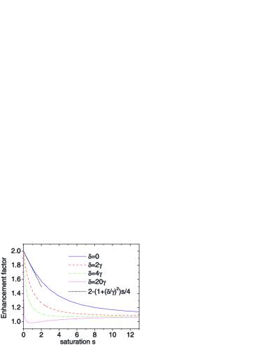
Figure 4: Numerical enhancement factor $\alpha$ in the helicity preserving channel $h\parallel h$, versus saturation $s$ of the atomic transition, for different detunings $\delta$ from resonant driving. Larger detuning leads to a faster loss of the CBS contrast. At small $s$, one recovers the perturbative prediction wellens04 linear in $s$ (straight dashed line). At large $s$, $\alpha$ saturates at a $\delta$-dependent value $\alpha_{\delta_{\infty}}>1$, due to the constructive self-interference of inelastically scattered photons. Remarkably, $\alpha$ also passes through a minimum at $s\simeq 0.5$, for very large detuning $\delta=20\gamma$. This indicates destructive interference, and the physical cause of this observation remains to be identified.

The enhancement factor $\alpha(s)$, Eq. (41), deduced from Eqs. (46,47) reads

$$\alpha(s)=1+\frac{R_{1}(s)}{(4+s)R_{2}(s)}\,,$$ (50)

and $\alpha(0)=2.0$ in the weak field limit, as expected. The dependence of $\alpha$ on the saturation parameter is shown in Fig. 4. As above for the individual cross and ladder terms, we again obtain perfect agreement with the linear decay predicted by the scattering theoretical result $\alpha\simeq 2-s/4$ wellens04 , in the limit of small $s$. When $s$ increases further, $\alpha$ monotonically drops to an asymptotic value $\lim_{s\to\infty}\alpha(s)=\alpha_{\infty}=23/21$ which is strictly larger than unity, implying a nonvanishing residual CBS contrast in the limit of large injected intensities. As we shall see further down in Sec. IV.1.3, this residual constructive interference effect is exclusively due to the (self-)interference of inelastically scattered photons.

IV.1.2 Finite detuning

It is in general no more possible to obtain explicit expressions for the Green’s matrix ${\bf G_{0}}$ (tantamount of inverting ${\bf A}$), in the case of nonvanishing detuning $\delta\neq 0$. However, this can always be done numerically, and Fig. 4 compares the enhancement factor at resonance to the one for three different nonvanishing values of $\delta$. In qualitative agreement with the experiment chaneliere03 , $\alpha$ decays faster for larger detuning, as $s$ is increased from zero. But not only does the enhancement factor exhibit a steeper (initial) decrease with $\delta$: it also reveals destructive interference ($\alpha<1$) for large detuning $\delta=20\gamma$, at $s\simeq 0.5$. This corresponds to a large Rabi frequency $\Omega\simeq 20\gamma$.

To gain some insight on whether such destructive interference is generic for large Rabi frequencies and large detunings, we monitor enhancement factor vs. detuning, for two fixed, large values of the Rabi frequency, as displayed in Fig. 5. For a given value of $\Omega$, the enhancement factor decreases as a function of $|\delta|$, from its maximum at $\delta=0$ to its $\Omega$-dependent minimum value at $|\delta|\simeq\Omega$. For very large detunings, $\alpha_{\delta}$ saturates at a level $1<\lim_{|\delta|\to\infty}=\alpha_{\delta_{\infty}}<\alpha_{\infty}$, indicating (i) constructive (self-)interference of far-detuned photons, and (ii) similar behavior of the ladder and crossed terms, asymptotically in $|\delta|$. The asymptotic value $\alpha_{\delta_{\infty}}$ is the lower the larger $\Omega$. Furthermore, as a direct counterpart of the destructive interference observed in Fig. 4, $\alpha$ drops below unity for $\Omega=20\gamma$, in a finite range of $|\delta|$.

Note that a similar effect was predicted in Kupriyanov04 , for linear double scattering from atoms with Zeeman-shifted hyperfine ground levels. In our case, the onset of destructive interference at $\delta\simeq 15\gamma$ and $s_{0}\simeq\Omega^{2}/2\gamma^{2}=200$ occurs approximately at saturation $s\simeq 0.9$. A physical interpretation of this interference-induced anti-enhancement of CBS, which we tentatively attribute to an AC-Stark shift of the laser-driven atomic sublevels, will require a closer inspection of the total stationary intensity, and is refered to a separate contribution.

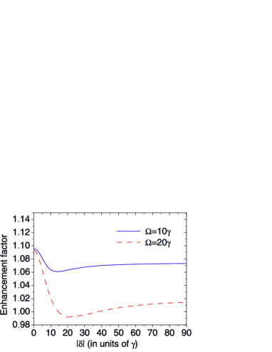
Figure 5: (Color online) Numerical enhancement factor $\alpha$ (numerical solution) in the helicity preserving channel, versus the laser detuning $\delta$, for two values of the driving Rabi frequency $\Omega$. The decrease of $\alpha$ below unity for $\Omega=20\gamma$, in the vicinity of $|\delta|=20\gamma$, correlates with the minimum displayed by $\alpha(s)$ in the corresponding plot in Fig. 4, at $s\simeq 0.5$.

IV.1.3 Elastic component at finite detuning

To see that the residual contrast observed in Fig. 4 for large saturation parameters stems from inelastically scattered photons, we now derive expressions for the elastic ladder and crossed contributions to the double scattering CBS signal. To do so, we extract the elastic contribution $I^{\rm el}_{2}$ to the total double scattering intensity from an expansion of Eq. (37) to second order in $|g|$, as prescribed by (34,35):

$$I^{\rm el}_{2}=|\langle\sigma^{1}_{21}\rangle^{[1]}_{\rm ss}|^{2}+|\langle\sigma^{2}_{21}\rangle^{[1]}_{\rm ss}|^{2}+2\,{\rm Re}\,\left(\langle\sigma^{1}_{21}\rangle^{[1]}_{\rm ss}\langle\sigma^{2}_{12}\rangle^{[1]}_{\rm ss}e^{i{\bf k}\cdot{\bf r}_{12}}\right)\,.$$ (51)

With the evolution equations

$$\dot{\langle\sigma^{\alpha}_{12}\rangle} = (-\gamma+i\delta)\langle\sigma^{\alpha}_{12}\rangle-\frac{i}{2}\Omega_{\alpha}\langle\sigma^{\alpha}_{42}\rangle$$ (52a)

$$+\sum_{i,j}T_{ij}\langle Q^{\alpha}_{i}Q^{\beta}_{j}\rangle,$$

$$\dot{\langle\sigma^{\alpha}_{42}\rangle} = -2\gamma\langle\sigma^{\alpha}_{42}\rangle-\frac{i}{2}\Omega^{*}_{\alpha}\langle\sigma^{\alpha}_{12}\rangle$$ (52b)

$$+\sum_{i,j}T_{ij}\langle Q^{\alpha}_{i}Q^{\beta}_{j}\rangle\,,$$

which can be derived from Eqs. (19-21), an analytic expression for the steady state mean value $\langle\sigma^{\alpha}_{12}\rangle^{[1]}_{\rm ss}$ and thus for $I^{\rm el}_{2}$ is obtained by the following argument (note that this remains valid also for finite detuning $\delta$): As long as we content ourselves with a lowest order treatment of multiple scattering effects, only factorized zeroth-order correlation functions $\langle Q^{\alpha}_{i}\rangle^{[0]}_{\rm ss}\langle Q^{\beta}_{j}\rangle^{[0]}_{\rm ss}$ for independent atoms $\alpha\neq\beta$ contribute to the sums on the rhs of Eqs. (52a,52b), since the coefficients $T_{ij}$ are of order $|g|$, expressing the dipole-dipole interaction between distinct atoms. Such products vanish except if their factors involve only the driven levels $\left|1\right\rangle_{\alpha}$ or $\left|4\right\rangle_{\beta}$. Consequently, the summations in Eqs. (52a) and (52b), which extend over different subsets of the two-atom correlation functions, can be condensed according to

$$\sum_{i,j}T_{ij}\langle Q^{\alpha}_{i}\rangle^{[0]}_{\rm ss}\langle Q^{\beta}_{j}\rangle^{[0]}_{\rm ss} \rightarrow \gamma g^{*}\overleftrightarrow{\boldsymbol{\Delta}}_{+1,+1}$$ (53)

$$\times\langle\sigma^{\beta}_{14}\rangle^{[0]}_{\rm ss}\langle\sigma^{\alpha}_{11}\rangle^{[0]}_{\rm ss},$$

$$\sum_{i,j}T_{ij}\langle Q^{\alpha}_{i}\rangle^{[0]}_{\rm ss}\langle Q^{\beta}_{j}\rangle^{[0]}_{\rm ss} \rightarrow \gamma g^{*}\overleftrightarrow{\boldsymbol{\Delta}}_{+1,+1}$$ (54)

$$\times\langle\sigma^{\beta}_{14}\rangle^{[0]}_{\rm ss}\langle\sigma^{\alpha}_{41}\rangle^{[0]}_{\rm ss}\,,$$

respectively. Substitution thereof into (52a,52b) (with the lhs of (52a,52b) equal to zero, and $\langle\sigma_{14}^{\alpha}\rangle=\langle\sigma_{41}^{\alpha}\rangle^{*}$), together with the known solutions of the optical Bloch equations for a single two-level atom cohen_tannoudji ,

$$\langle\sigma^{\alpha}_{14}\rangle_{\rm ss}^{[0]}=\frac{i(\gamma+i\delta)}{\Omega_{\alpha}^{*}}\frac{s}{1+s},\quad\langle\sigma^{\alpha}_{11}\rangle_{\rm ss}^{[0]}=\frac{2+s}{2(1+s)}\,,$$ (55)

leads to

$$\langle\sigma^{\alpha}_{12}\rangle^{[1]}_{\rm ss}=\frac{i\gamma g^{*}\overleftrightarrow{\boldsymbol{\Delta}}_{+1,+1}\Omega_{\beta}}{2(\gamma-i\delta)^{2}(1+s)^{2}}\,.$$ (56)

If we now rewrite Eq. (51) as

$$I^{\rm el}_{2}=|T_{\rm dir}+T_{\rm rev}|^{2},$$ (57)

with $T_{\rm dir}\equiv\langle\sigma^{1}_{12}\rangle^{[1]}_{\rm ss}e^{-i{\bf k}\cdot{\bf r}_{1}}$ and $T_{\rm rev}\equiv\langle\sigma^{2}_{12}\rangle^{[1]}_{\rm ss}e^{-i{\bf k}\cdot{\bf r}_{2}}$, the elastic component of the double scattering intensity appears, with (11), as the square modulus of a sum of the ‘direct’ and ‘reversed’ scattering amplitudes

$$T_{\rm dir} = \frac{i\gamma g^{*}\overleftrightarrow{\boldsymbol{\Delta}}_{+1,+1}\Omega}{2(\gamma-i\delta)^{2}(1+s)^{2}}e^{i{\bf k}_{L}\cdot{\bf r}_{2}-i{\bf k}\cdot{\bf r}_{1}},$$ (58)

$$T_{\rm rev} = \frac{i\gamma g^{*}\overleftrightarrow{\boldsymbol{\Delta}}_{+1,+1}\Omega}{2(\gamma-i\delta)^{2}(1+s)^{2}}e^{i{\bf k}_{L}\cdot{\bf r}_{1}-i{\bf k}\cdot{\bf r}_{2}}\,.$$ (59)

Direct and reverse amplitude are symmetric under the interchange ${\bf k}\leftrightarrow-{\bf k}_{L}$, and thus satisfy the condition of reciprocity jonckheere00 . Consequently, the elastically scattered photons remain strictly coherent, for any $s$, and show perfect CBS contrast with $\alpha(s)=2$, as immediately spelled out by the explicit expression for the elastic ladder and crossed terms, at arbitrary detuning and Rabi frequency:

$$L^{\rm el}_{2}=C^{\rm el}_{2}(0)=\frac{2|\tilde{g}|^{2}}{15}\frac{1}{1+(\delta/\gamma)^{2}}\frac{s}{(1+s)^{4}}\,.$$ (60)

While perfectly coherent even for large $s$, the elastic contribution to the total double scattering intensity decreases as $s^{-3}$, by virtue of Eq. (60), after passing through a maximum at $s=1/3$. In contrast, the total signal fades away like $s^{-1}$, according to Eqs. (46,47). Consequently, in the large $s$ limit, the CBS signal is completely dominated by the inelastic scattering component, and the residual CBS contrast $\alpha_{\infty}$ observed in Sec. IV.1.1 above is due to the selfinterference of inelastically scattered photons, which are incoherent with respect to the injected laser radiation. The visibility of this residual interference signal is limited by the amount of which-way information communicated to the environment, during the multiple scattering process Englert96 .

Finally, let us note that equation (60) allows for a transparent interpretation, since it can be factorized into

• the elastic intensity

  $$I^{\rm el[0]}\propto\frac{s}{(1+s)^{2}}$$ (61)

  scattered by the first strongly driven atom,

• the total scattering cross section

  $$\sigma^{\rm tot}\propto\frac{1}{(1+(\delta/\gamma)^{2})(1+s)}$$ (62)

  of the second atom, and

• the relative weight $I^{\rm el[0]}/I^{\rm tot[0]}=\sigma^{\rm el}/\sigma^{\rm tot}$ equal to

  $$\frac{\gamma^{2}+\delta^{2}}{\gamma^{2}+\Omega^{2}/2+\delta^{2}}=\frac{1}{1+s}$$ (63)

  of elastic processes cohen_tannoudji .

IV.2 $lin\perp lin$ channel

Up to a constant factor $1/2$, the results for the $lin\perp lin$ channel turn out to be the same as for the $h\parallel h$ channel, at exact backscattering. For a given value of $s$, the ladder and crossed terms are two times smaller than in the $h\parallel h$ channel. Since, however, Eq. (16) for the intensity in the $lin\perp lin$ channel is manifestly different from Eq. (15), the $h\parallel h$ result, a short discussion of this observation is in order.

In both cases, the CBS intensity is observed in the polarization channel orthogonal to the excitation channel. In the $h\parallel h$ channel, the orthogonal channel is defined by one dipole transition $|2\rangle\rightarrow|1\rangle$. In the $lin\perp lin$ channel, the orthogonal channel is defined by two atomic transitions, $|2\rangle\rightarrow|1\rangle$ and $|4\rangle\rightarrow|1\rangle$. Yet, by introducing a superposition state $|e\rangle\equiv|2\rangle+|4\rangle$, we can rewrite expression (16) in a way which is formally equivalent to (15). However, the geometric weight of the resulting ladder and crossed intensities is given by $(\overleftrightarrow{\boldsymbol{\Delta}}_{0,-1}+\overleftrightarrow{\boldsymbol{\Delta}}_{0,+1})(\overleftrightarrow{\boldsymbol{\Delta}}_{+1,0}+\overleftrightarrow{\boldsymbol{\Delta}}_{-1,0})/2$. Only two of these four terms, $\overleftrightarrow{\boldsymbol{\Delta}}_{0,-1}\overleftrightarrow{\boldsymbol{\Delta}}_{-1,0}/2$ and $\overleftrightarrow{\boldsymbol{\Delta}}_{0,+1}\overleftrightarrow{\boldsymbol{\Delta}}_{+1,0}/2$, survive the configuration average, what leads to results that are two times smaller than in the $h\parallel h$ channel.

IV.3 $h\perp h$ channel

We shall now consider detected photons which have the same polarization as the incident ones. Hence, as already briefly discussed in Sec. II.6, single scattering as well as double scattering events will contribute to the detected signal, with the latter only a small correction to the former. Correspondigly, an experimental detection of the double scattering contribution alone is excluded. Nonetheless, it is instructive to consider this scenario in the regime of a nonlinear atomic response to the injected radiation because it allows to identify the role of recurrent scattering where one photon rescatters from the same atom, after visiting the other (this process is second order in the coupling constant $|g|$).

IV.3.1 Total intensity

To obtain explicit expressions for the total scattered intensity, we proceed stepwise and first expand the single atom contribution to the intensity, in Eq. (17), to second order in $g$. We obtain

$$\sum_{\alpha=1}^{2}\langle\sigma_{44}^{\alpha}\rangle_{\rm ss}^{[2]} = |g|^{2}\left[F_{1}(s)|\overleftrightarrow{\boldsymbol{\Delta}}_{+1,-1}|^{2}\right.$$

$$\left.+F_{2}(s)(|\overleftrightarrow{\boldsymbol{\Delta}}_{+1,0}|^{2}+|\overleftrightarrow{\boldsymbol{\Delta}}_{+1,+1}|^{2})\right]$$

$$+\;{\rm terms}\;\propto\,{\rm Re}\,[g^{2}]\,,|g|^{2}\cos\{2{\bf k}_{L}\cdot{\bf r}_{12}\}\,,$$

where

$$F_{1}(s) = \frac{36s+3s^{2}-27s^{3}-19s^{4}-s^{5}}{12(1+s)^{5}(3+s)}\,,$$ (65)

$$F_{2}(s) = -\frac{4s^{2}(288+132s+23s^{2}+s^{3})}{3(1+s)P(s)}\,,$$ (66)

with $P(s)$ from Eq. (44). The terms in the last line of (IV.3.1) oscillate rapidly on the typical scale $\ell$ of the interatomic separation (recall Eq. (22), and $k_{0}r_{\alpha\beta}\gg 1$; this is, also the dependence of $g$ on $r_{12}$ is to be taken into account here), and average out under the integral over $r_{12}$ in (38). Thus, they will be dropped hereafter, whereas terms $\propto|g|^{2}=9/4k_{0}^{2}r_{12}^{2}$ vary smoothly with $r_{12}$, and will be kept.

An analogous expansion of the interference terms in (17) yields the expression

$$2\,{\rm Re}\,\{\langle\sigma_{41}^{1}\sigma_{14}^{2}\rangle_{\rm ss}^{[2]}e^{i{\bf k}\cdot{\bf r}_{12}}\} = |g|^{2}F_{3}(s)|\overleftrightarrow{\boldsymbol{\Delta}}_{+1,-1}|^{2}$$

$$\times\cos\{({\bf k}+{\bf k}_{L})\cdot{\bf r}_{12}\}$$

$$+\;{\rm terms}\;\propto\,{\rm Re}\,[g^{2}]\,,$$

$$\;\;\;|g|^{2}\cos\{({\bf k}-{\bf k}_{L})\cdot{\bf r}_{12}\}\,,$$

$$\;\;\;|g|^{2}\cos\{(3{\bf k}_{L}-{\bf k})\cdot{\bf r}_{12}\}\,,$$

where

$$F_{3}(s)=\frac{324s+540s^{2}+450s^{3}+219s^{4}+85s^{5}+29s^{6}+s^{7}}{36(1+s)^{6}(3+s)^{2}}\,.$$ (68)

The three last lines of Eq. (IV.3.1) are irrelevant for our subsequent treatment, for exactly the same reason as the corresponding terms in Eq. (IV.3.1).

We now have a closer look at the geometric factors in these equations, which allow the identification of the underlying elementary scattering processes. The geometric weight of the contribution proportional to $F_{2}(s)$ in (IV.3.1) is given by $|\overleftrightarrow{\boldsymbol{\Delta}}_{+1,0}|^{2}+|\overleftrightarrow{\boldsymbol{\Delta}}_{+1,+1}|^{2}$. It describes the coupling of a photon from the $\left|4\right\rangle_{\alpha}\rightarrow\left|1\right\rangle_{\alpha}$ transition to either the $\left|3\right\rangle_{\beta}\rightarrow\left|1\right\rangle_{\beta}$, or to the $\left|2\right\rangle_{\beta}\rightarrow\left|1\right\rangle_{\beta}$ transition, respectively, then back to the $\left|4\right\rangle_{\alpha}\rightarrow\left|1\right\rangle_{\alpha}$ transition, and only then to a detector. This is recurrent scattering. (Note that non-recurrent transitions, e.g., from $\left|4\right\rangle_{\alpha}\rightarrow\left|1\right\rangle_{\alpha}$ to $\left|3\right\rangle_{\beta}\rightarrow\left|1\right\rangle_{\beta}$ or to $\left|2\right\rangle_{\beta}\rightarrow\left|1\right\rangle_{\beta}$ cannot give rise to a detected photon in the $h\perp h$ channel.)

More precisely, the single scattering contribution with the weight $F_{2}(s)$ originates from the interference between single scattering from independent atoms and (recurrent) triple scattering, in which a photon is subsequently scattered by atom $\alpha$, then by atom $\beta$, and by atom $\alpha$ again (recall our discussion in Sec. II.6, and also see Eqs. (IV.3.2,IV.3.2) in our subsequent discussion of the elastic contribution to the $h\perp h$ channel). Since the rate of single and recurrent scattering is equally limited by the number of photons incident on the atom, $\propto s$, it follows that $F_{2}(s)\propto s^{2}$ for $s\rightarrow 0$. This is consistent with a basic postulate of multiple scattering theory tiggelen96 , according to which recurrent scattering is irrelevant in the linear regime of weak saturation. It is also clear why there is no recurrent scattering in $h\parallel h$ and $lin\perp lin$ channels: Indeed, single scattering is essential for recurrent scattering to show up at order $|g|^{2}$, but is filtered out in the orthogonal polarization channels.

Now consider those terms in Eqs. (IV.3.1) and (IV.3.1) with angular part $|\overleftrightarrow{\boldsymbol{\Delta}}_{+1,-1}|^{2}$. Along with the processes in which atoms exchange photons, these equally much represent the two recurrent scattering sequences $\left|4\right\rangle_{\alpha}\rightarrow\left|4\right\rangle_{\beta}\rightarrow\left|4\right\rangle_{\alpha}$. The weight of these contributions is not the same as for $\left|4\right\rangle_{\alpha}\rightarrow\left|3\right\rangle_{\beta}\rightarrow\left|4\right\rangle_{\alpha}$ and $\left|4\right\rangle_{\alpha}\rightarrow\left|2\right\rangle_{\beta}\rightarrow\left|4\right\rangle_{\alpha}$ transitions, since the presence of the driving field in the $\left|1\right\rangle\leftrightarrow\left|4\right\rangle$ transition definitely destroys the symmetry of the excited state sublevels.

As regards the sign of the various scattering contributions in Eqs. (IV.3.1,IV.3.1), note that the weight of the interference part given by Eq. (68) is positive for all $s$, while $F_{1}(s)$ and $F_{2}(s)$, Eqs. (65,66), are nonpositive, the function $F_{2}(s)$ being strictly negative for $s\neq 0$. Hence, recurrent scattering is a small negative correction to the overall positive single-atom contribution to the total scattering signal.

The total crossed and ladder contributions to the double scattering intensity are once again obtained after a final configuration average of Eqs. (IV.3.1) and (IV.3.1):

$$L^{\rm tot}_{2} = \frac{1}{15}|\tilde{g}|^{2}(7F_{1}(s)+3F_{2}(s))\,,$$ (69)

$$C^{\rm tot}_{2}(0) = \frac{7}{15}|\tilde{g}|^{2}F_{3}(s)\,.$$ (70)

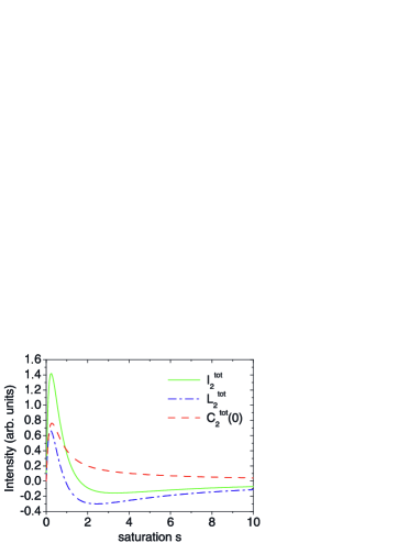
Figure 6: (Color online) Total crossed (Eqs. (70)) and ladder (Eq. (69)) terms, together with the double scattering intensity $I_{2}^{\rm tot}=L_{2}^{\rm tot}+C_{2}^{\rm tot}(0)$, in the $h\perp h$ channel, as functions of the saturation $s$, at exact resonance $\delta=0$.

The result is plotted in Fig. 6, where $L^{\rm tot}_{2}$ turns negative in a finite interval of $s$. In the limit of large $s$, the ladder term approaches zero from below, as $1/s$, whereas the crossed terms decreases towards zero, with the same rate $1/s$. Note that the negativity of the ladder term is compensated for by the single scattering contribution $L_{1}$ which cannot be separated from the double scattering contribution, in the $h\perp h$ channel. Furthermore, the single scattering contribution does not decrease with growing $s$ but rather saturates, so that for very large saturation parameters we can simply ignore the double scattering contribution. For all $s$, the CBS enhancement factor reads, after inclusion of $L_{1}$:

$$\alpha=1+\frac{C^{\rm tot}_{2}(0)}{L_{1}+L^{\rm tot}_{2}}\,.$$ (71)

In a real medium, the relative weight of single and double scattering depends on the optical thickness. However, our simple model cannot correctly account for this effect; hence, we cannot assess here whether the negativity of the double scattering ladder term has observable consequences in laboratory experiments.

IV.3.2 Elastic component

Let us finally extract the elastic component of the CBS intensiy in the $h\perp h$ channel. According to (17) and (36), with (38), the elastic ladder and crossed terms are given by

$$L^{\rm el}_{2} = 2\left\langle|\langle\sigma_{41}^{1}\rangle^{[1]}_{\rm ss}|^{2}\right.$$

$$\left.+\langle\sigma^{1}_{41}\rangle^{[0]}_{\rm ss}\langle\sigma^{1}_{14}\rangle^{[2]}_{\rm ss}+\langle\sigma^{1}_{41}\rangle^{[2]}_{\rm ss}\langle\sigma^{1}_{14}\rangle^{[0]}_{\rm ss}\right\rangle_{\rm conf}\,,$$

$$C^{\rm el}_{2}(\theta) = 2\,{\rm Re}\,\left\langle e^{i\textbf{k}\cdot{\bf r}_{12}}\left(\langle\sigma^{1}_{41}\rangle^{[1]}_{\rm ss}\langle\sigma^{2}_{14}\rangle^{[1]}_{\rm ss}\right.\right.$$

$$\left.\left.+\langle\sigma^{1}_{41}\rangle^{[0]}_{\rm ss}\langle\sigma^{2}_{14}\rangle^{[2]}_{\rm ss}+\langle\sigma^{1}_{41}\rangle^{[2]}_{\rm ss}\langle\sigma^{2}_{14}\rangle^{[0]}_{\rm ss}\right)\right\rangle_{\rm conf}\,.$$

Due to the factorization (36) of the classically radiating dipoles, symmetric and asymmetric scattering contributions are directly born out: Products of first order (labeled by ‘$[1]$’) contributions in $g$ represent double scattering of photons subsequently at atoms $1$ and $2$, in direct and reversed order, whereas products of zero and second order (‘$[0]$’ and ‘$[2]$’, respectively) express indistinguishable single scattering and recurrent scattering amplitudes upon either one of the atoms. Explicitly, the above expressions have the following geometric weights,

$$L^{\rm el}_{2} = \left\langle|g|^{2}|\overleftrightarrow{\boldsymbol{\Delta}}_{+1,-1}|^{2}\right\rangle_{\rm conf}\times\left[\frac{s+s^{3}}{(1+s)^{6}}+F_{4}(s)\right]$$ (74)

$$+\left\langle|g|^{2}(|\overleftrightarrow{\boldsymbol{\Delta}}_{+1,0}|^{2}+|\overleftrightarrow{\boldsymbol{\Delta}}_{+1,+1}|^{2})\right\rangle_{\rm conf}$$

$$\times\frac{2F_{2}(s)}{1+s}\,,$$

$$C^{\rm el}_{2}(\theta) = \left\langle|g|^{2}|\overleftrightarrow{\boldsymbol{\Delta}}_{+1,-1}|^{2}\cos\{({\bf k}+{\bf k}_{L})\cdot{\bf r}_{12}\}\right\rangle_{\rm conf}$$ (75)

$$\times\left[\frac{s}{(1+s)^{6}}+F_{5}(s)\right]\,$$

where all terms which vanish under the configuration average have already been dropped (see also the discussion of Eqs. (IV.3.1,IV.3.1) above), and

$$F_{4}(s) = \frac{-36s^{2}-39s^{3}-14s^{4}+s^{5}}{3(1+s)^{6}(3+s)}\,,$$ (76)

$$F_{5}(s) = \frac{-72s^{2}-51s^{3}-s^{4}+3s^{5}+s^{6}}{12(1+s)^{6}(3+s)}\,.$$ (77)

Upon evaluation of the configuration average, we obtain the final result

$$L^{\rm el}_{2} = |\tilde{g}|^{2}\frac{7}{15}\left[\frac{s+s^{3}}{(1+s)^{6}}+F_{4}(s)+\frac{6}{7}\frac{F_{2}(s)}{1+s}\right]\,,$$ (78)

$$C^{\rm el}_{2}(0) = |\tilde{g}|^{2}\frac{7}{15}\left[\frac{s}{(1+s)^{6}}+F_{5}(s)\right]\,.$$ (79)

Expressions (78) and (79) imply that, in the small-$s$ limit, the elastic ladder and crossed terms coincide, as for orthogonal polarization channels (see Eq. (60)). However, this equipartition does not prevail here beyond the linear regime, due to reciprocity violating processes wellens04 which lead to a deviation of $L^{\rm el}_{2}$ from $C^{\rm el}_{2}(0)$, already at quadratic order in $s$. The violation of reciprocity was originally demonstrated in wellens04 for scalar atoms, and it will be demonstrated below in Sect. IV.5 that the scalar results immediately follow from our present results for parallel excitation/detection polarization channels, when ignoring those electronic sublevels that mediate recurrent scattering. However, beyond those reciprocity-violating processes already implicit in the scalar treatment, other processes specifically due to the vector character of the injected radiation field lead to additional deviations (expressed by the term $\propto F_{2}(s)$ in (78)).

Furthermore, note that the elastic ladder and crossed intensities in the $h\perp h$ channel asymptotically behave like $\propto 1/s^{2}$ and $\propto 1/s$, respectively. Also the total double scattering intensity in this channel is characterized by an asymptotic decrease $\propto 1/s$ (see Sec. IV.3.1). Consequently, unlike the $h\parallel h$ channel, where double scattering becomes purely inelastic for large $s$, here both, elastic and inelastic photons, are present for large $s$.

IV.4 $lin\parallel lin$ channel

The results for the $lin\parallel lin$ channel are the same as for the $h\perp h$ channel, modulo the following substitution of the geometric weights:

$$|\overleftrightarrow{\boldsymbol{\Delta}}_{+1,-1}|^{2}\rightarrow|\overleftrightarrow{\boldsymbol{\Delta}}_{0,0}|^{2},\quad|\overleftrightarrow{\boldsymbol{\Delta}}_{+1,+1}|^{2}\rightarrow|\overleftrightarrow{\boldsymbol{\Delta}}_{-1,0}|^{2}.$$ (80)

This entails slightly different final expressions for the ladder and crossed terms. For the total intensities, we obtain

$$L^{\rm tot}_{2} = \frac{1}{15}|\tilde{g}|^{2}[8F_{1}(s)+2F_{2}(s)]\,,$$ (81)

$$C^{\rm tot}_{2}(0) = \frac{8}{15}|\tilde{g}|^{2}F_{3}(s)\,,$$ (82)

and the elastic result reads

$$L^{\rm el}_{2} = |\tilde{g}|^{2}\frac{8}{15}\Bigl{[}\frac{s+s^{3}}{(1+s)^{6}}+\frac{F_{2}(s)}{2(1+s)}+F_{4}(s)\Bigr{]}\,,$$ (83)

$$C^{\rm el}_{2}(0) = |\tilde{g}|^{2}\frac{8}{15}\Bigl{[}\frac{s}{(1+s)^{6}}+F_{5}(s)\Bigr{]}\,.$$ (84)

Eqs. (81,82) and (83,84) differ from (69,70) and (78,79) only through numerical coefficients. Therefore, all our above conclusions for the elastic and inelastic components of double scattering in the $h\perp h$ channel also apply for the present $lin\parallel lin$ case.

IV.5 Scattering of scalar photons on a two-level atom

To conclude, let us briefly consider the model scenario of scalar photons scattering on a two-level atom – a wide-spread setting in typical quantum optical model calculations, which neglects the important role of the polarization degree of freedom in the presently discussed quantum transport problem. The scalar case is easily deduced from the above results for the $h\perp h$ or $lin\parallel lin$ channels, by simply setting equal to zero those contributions with the geometric weight $|\overleftrightarrow{\boldsymbol{\Delta}}_{+1,0}|^{2}+|\overleftrightarrow{\boldsymbol{\Delta}}_{+1,+1}|^{2}$ – since a two-level atom does not offer the required atomic transitions.

The total ladder and crossed terms then read, by virtue of Eqs. (IV.3.1,IV.3.1,69,70),

$$L^{\rm tot}_{2} = \frac{7}{15}|\tilde{g}|^{2}F_{1}(s)\,,$$ (85)

$$C^{\rm tot}_{2}(0) = \frac{7}{15}|\tilde{g}|^{2}F_{3}(s)\,,$$ (86)

with the quadratic expansion

$$L^{\rm tot}_{2}\propto s-\frac{21}{4}s^{2}\,,\quad C^{\rm tot}_{2}(0)\propto s-5s^{2}\,,$$ (87)

in precise agreement with the result of wellens04 .

Correspondingly, the elastic contributions, Eqs. (78,79), reduce to

$$L^{\rm el}_{2} = |\tilde{g}|^{2}\frac{7}{15}\Bigl{[}\frac{s+s^{3}}{(1+s)^{6}}+F_{4}(s)\Bigr{]}\,,$$ (88)

$$C^{\rm el}_{2}(0) = |\tilde{g}|^{2}\frac{7}{15}\Bigl{[}\frac{s}{(1+s)^{6}}+F_{5}(s)\Bigr{]}\,,$$ (89)

which once again reproduces the second order expression

$$L^{\rm el}_{2}\propto s-10s^{2},\quad C^{\rm el}_{2}(0)\propto s-8s^{2}.$$ (90)

of wellens04 .

Thus, the scalar model correctly predicts the maximum enhancement factor $\alpha=2$, in the elastic scattering limit $s\to 0$. Furthermore, it correctly describes those CBS contributions in the parallel excitation/detection channels which originate from the laser driven transitions, for arbitrary $s$. However, the scalar model in general leads to incorrect results, since it ignores contributions from those sublevels of the degenerate excited state which are not driven by the laser, yet mediate recurrent scattering, as we have seen in Sec. IV.3.1.

V Summary

In summary, we have given detailed account of the master equation treatment of coherent backscattering of light from a disordered sample of cold atoms with a nondegenerate electronic ground state. This approach extracts all physical observables from the steady state expectation values of atomic dipole operators. Furthermore, our treatment incorporates, to the best of our knowledge for the first time, the effect of interatomic dipole-dipole interactions for distant atoms.

In particular, the formalism allows to treat arbitrary pump intensities which possibly saturate the relevant atomic transitions, thus leading to inelastic scattering events (when more than one photon is incident on the scattering atom – on the spectral level, this entails the emergence of the famous Mollow triplet, in a single atom’s fluorescence). The price to pay is a rapidly increasing dimension of the Hilbert space spanned by the many atoms’ degrees of freedom. This limited our present treatment to two atomic scatterers, which is the minimum number of constituents to observe the CBS effect. Nonetheless, this approach allowed us to show that a small residual CBS signal survives even in the limit of purely inelastic scattering, due to the self-interference of inelastically scattered photons.

Furthermore, we have seen that recurrent scattering leads to a reduction of the total double scattering signal, due to a destructive interference between single and triple scattering events upon the same atomic scatterer.

Another advantage of the master equation treatment presented here, so far unexplored, is the immediate availability of the CBS spectrum through a Fourier transform of suitable atomic dipole correlation functions, as well as of the associated photocount statistics. Whether CBS has an unambiguous signature in the spectrum and/or in the photocurrent remains hitherto an open question, but is getting in reach for state of the art experiments.

It is a pleasure to acknowledge entertaining and enlightening discussions with Dominique Delande, Benoît Grémaud, Christian Miniatura, and Thomas Wellens.

References

- (1) E. Akkermans, G. Montambaux, J.-L. Pichard, and J. Zinn-Justin (Eds.) Mesoscopic Quantum Physics (Elsevier, Amsterdam, 1994).
- (2) P. Sheng, Introduction to Wave Scattering, Localization and Mesoscopic Phenomena (Academic Press, San Diego, 1995).
- (3) Y. Kuga and A. Ishimaru, J. Opt. Soc. Am. A 1, 831 (1984); M. P. van Albada and A. Lagendijk, Phys. Rev. Lett. 55, 2692 (1985); P. E. Wolf and G. Maret, ibid. 2996.
- (4) G. Labeyrie, F. de Tomasi, J.-C. Bernard, C. A. Müller, C. Miniatura and R. Kaiser, Phys. Rev. Lett. 83, 5266 (1999).
- (5) P. Katalunga, C. I. Sukenik, S. Balik, M. D. Havey, D. V. Kupriyanov, and I. M. Sokolov, Phys. Rev. A68, 033816 (2003).
- (6) T. Chanelière, D. Wilkowski, Y. Bidel, R. Kaiser, and C. Miniatura, Phys. Rev. E70, 036602 (2004).
- (7) C. A. Müller and C. Miniatura, J.Phys. A 35, 10163 (2002).
- (8) C. Cohen-Tannoudji, J. Dupont-Roc, G. Grynberg, Atom-Photon Interactions (John Wiley & Sons Inc, New York, 1992).
- (9) H. Cao, Y. Ling, J. Y. Xu, C. Q. Cao, and Prem Kumar, Phys. Rev. Lett. 86, 4524 (2001).
- (10) G. Labeyrie, D. Delande, C. A. Müller, C. Miniatura, and R. Kaiser, Europhys. Lett. 61, 327 (2003).
- (11) T. Wellens, B. Grémaud, D. Delande, and C. Miniatura, Phys. Rev. A70, 023817 (2004).
- (12) B. Grémaud, T. Wellens, D. Delande, C. Miniatura, arXiv:quant-ph/0506010.
- (13) V. Shatokhin, C. A. Müller, and A. Buchleitner, Phys. Rev. Lett. 94, 043603 (2005).
- (14) H. J. Carmichael, An open system approach to quantum optics (Springer, New-York, 1993).
- (15) R. H. Lehmberg, Phys. Rev. A 2, 883 (1970); D. F. V. James, ibid. 47, 1336 (1993); J. Guo and J. Cooper, ibid. 51, 3128 (1995).
- (16) In the above, and have to be read as dyadic products.
- (17) T. Jonckheere, C. A. Müller, R. Kaiser, C. Miniatura, and D. Delande, Phys. Rev. Lett. 85, 4269 (2000).
- (18) Y. Bidel, B. Klappauf, J. C. Bernard, D. Delande, G. Labeyrie, C. Miniatura, D. Wilkowski, and R. Kaiser, Phys. Rev. Lett. 88, 203902 (2002).
- (19) A. Lagendijk and B. A. van Tiggelen, Phys. Rep. 270, 143 (1996).
- (20) D. S. Wiersma, M. P. van Albada, B. A. van Tiggelen, and A. Lagendijk, Phys. Rev. Lett. 74, 4193 (1995).
- (21) C. A. Müller, T. Jonckheere, C. Miniatura, and D. Delande, Phys. Rev. A 64, 053804 (2001).
- (22) D.V. Kupriyanov, I.M. Sokolov, and M.D. Havey Opt. Comm. 243, 165 (2004)
- (23) B.-G. Englert, Phys. Rev. Lett. 77, 2154 (1996).