The Projective Line Over the Finite Quotient Ring GF(2)[$x$]/$\langle x^{3}-x\rangle$ and Quantum Entanglement
I. Theoretical Background

Metod Saniga^† and Michel Planat^‡

Abstract

The paper deals with the projective line over the finite factor ring $R_{\clubsuit}\equiv$ GF(2)[$x$]/$\langle x^{3}-x\rangle$. The line is endowed with 18 points, spanning the neighbourhoods of three pairwise distant points. As $R_{\clubsuit}$ is not a local ring, the neighbour (or parallel) relation is not an equivalence relation so that the sets of neighbour points to two distant points overlap. There are nine neighbour points to any point of the line, forming three disjoint families under the reduction modulo either of two maximal ideals of the ring. Two of the families contain four points each and they swap their roles when switching from one ideal to the other; the points of the one family merge with (the image of) the point in question, while the points of the other family go in pairs into the remaining two points of the associated ordinary projective line of order two. The single point of the remaining family is sent to the reference point under both the mappings and its existence stems from a non-trivial character of the Jacobson radical, ${\cal J}_{\clubsuit}$, of the ring. The factor ring $\widetilde{R}_{\clubsuit}\equiv R_{\clubsuit}/{\cal J}_{\clubsuit}$ is isomorphic to GF(2) $\otimes$ GF(2). The projective line over $\widetilde{R}_{\clubsuit}$ features nine points, each of them being surrounded by four neighbour and the same number of distant points, and any two distant points share two neighbours. These remarkable ring geometries are surmised to be of relevance for modelling entangled qubit states, to be discussed in detail in Part II of the paper.

Keywords: Projective Ring Lines – Finite Quotient Rings – Neighbour/Distant Relation
                 Quantum Entanglement

1 Introduction

Geometries over rings instead of fields have been investigated by numerous authors for a long time [1], yet they have only recently been employed in physics [2] and found their potential applications in other natural sciences as well [3]. The most prominent, and at first sight rather counter-intuitive, feature of ring geometries (of dimension two and higher) is the fact that two distinct points/lines need not have a unique connecting line/meeting point [4]–[7]. Perhaps the most elementary, best-known and most thoroughly studied ring geometry is a finite projective Hjelmslev plane [2], [8]–[12].

Various ring geometries differ from each other essentially by the properties imposed on the underlying ring of coordinates. In the present paper we study the structure of the projective line defined over a finite quotient ring $R_{\clubsuit}\equiv$ GF(2)[$x$]/$\langle x^{3}-x\rangle$. Such a ring is, like those employed in [2] and [3], close enough to a field to be handled effectively, yet rich enough in its structure of zero-divisors for the corresponding geometry to be endowed with a non-trivial structure when compared with that of field geometries and to yield interesting and important applications in quantum physics, dovetailing nicely with those discussed in [2] and [3].

2 Basics of Ring Theory

In this section we recollect some basic definitions and properties of rings that will be employed in the sequel and to the extent that even the reader not well-versed in the ring theory should be able to follow the paper without the urgent need of consulting further relevant literature (e.g., [13]–[15]).

A ring is a set $R$ (or, more specifically, ($R,+,*$)) with two binary operations, usually called addition ($+$) and multiplication ($*$), such that $R$ is an abelian group under addition and a semigroup under multiplication, with multiplication being both left and right distributive over addition. A ring in which the multiplication is commutative is a commutative ring. A ring $R$ with a multiplicative identity 1 such that 1$r$ = $r$1 = $r$ for all $r\in R$ is a ring with unity. A ring containing a finite number of elements is a finite ring. In what follows the word ring will always mean a commutative ring with unity.

An element $r$ of the ring $R$ is a unit (or an invertible element) if there exists an element $r^{-1}$ such that $rr^{-1}=r^{-1}r=1$. This element, uniquely determined by $r$, is called the multiplicative inverse of $r$. The set of units forms a group under multiplication. A (non-zero) element $r$ of $R$ is said to be a (non-trivial) zero-divisor if there exists $s\neq 0$ such that $sr=rs=0$. An element of a finite ring is either a unit or a zero-divisor. A ring in which every non-zero element is a unit is a field; finite (or Galois) fields, often denoted by GF($q$), have $q$ elements and exist only for $q=p^{n}$, where $p$ is a prime number and $n$ a positive integer. The smallest positive integer $s$ such that $s1=0$, where $s1$ stands for $1+1+1+\ldots+1$ ($s$ times), is called the characteristic of $R$; if $s1$ is never zero, $R$ is said to be of characteristic zero.

An ideal ${\cal I}$ of $R$ is a subgroup of $(R,+)$ such that $a{\cal I}={\cal I}a\subseteq{\cal I}$ for all $a\in R$. An ideal of the ring $R$ which is not contained in any other ideal but $R$ itself is called a maximal ideal. If an ideal is of the form $Ra$ for some element $a$ of $R$ it is called a principal ideal, usually denoted by $\langle a\rangle$. A ring with a unique maximal ideal is a local ring. Let $R$ be a ring and ${\cal I}$ one of its ideals. Then $\overline{R}\equiv R/{\cal I}=\{a+{\cal I}~{}|~{}a\in R\}$ together with addition $(a+{\cal I})+(b+{\cal I})=a+b+{\cal I}$ and multiplication $(a+{\cal I})(b+{\cal I})=ab+{\cal I}$ is a ring, called the quotient, or factor, ring of $R$ with respect to ${\cal I}$; if ${\cal I}$ is maximal, then $\overline{R}$ is a field. A very important ideal of a ring is that represented by the intersection of all maximal ideals; this ideal is called the Jacobson radical.

A mapping $\pi$:  $R\mapsto S$ between two rings $(R,+,*)$ and $(S,\oplus,\otimes)$ is a ring homomorphism if it meets the following constraints: $\pi(a+b)=\pi(a)\oplus\pi(b)$, $\pi(a*b)=\pi(a)\otimes\pi(b)$ and $\pi(1)=1$ for any two elements $a$ and $b$ of $R$. From this definition it is readily discerned that $\pi(0)=0$, $\pi(-a)=-\pi(a)$, a unit of $R$ is sent into a unit of $S$ and the set of elements $\{a\in R~{}|~{}\pi(a)=0\}$, called the kernel of $\pi$, is an ideal of $R$. A canonical, or natural, map $\overline{\pi}$: $R\rightarrow\overline{R}\equiv R/{\cal I}$ defined by $\overline{\pi}(r)=r+{\cal I}$ is clearly a ring homomorphism with kernel ${\cal I}$. A bijective ring homomorphism is called a ring isomorphism; two rings $R$ and $S$ are called isomorphic, denoted by $R\cong S$, if there exists a ring isomorphism between them.

Finally, we mention a couple of relevant examples of rings: a polynomial ring, $R[x]$, viz. the set of all polynomials in one variable $x$ and with coefficients in a ring $R$, and the ring $R_{\otimes}$ that is a (finite) direct product of rings, $R_{\otimes}\equiv R_{1}\otimes R_{2}\otimes\ldots\otimes R_{n}$, where the component rings need not be the same.

3 The Ring $R_{\clubsuit}$ and Its Canonical Homomorphisms

The ring $R_{\clubsuit}\equiv$ GF(2)[$x$]/$\langle x^{3}-x\rangle$ is, like GF(2) itself, of characteristic two and consists of the following $\#_{{\rm t}}=8$ elements

$$R_{\clubsuit}=\{0,1,x,x+1,x^{2},x^{2}+1=(x+1)^{2},x^{2}+x,x^{2}+x+1\}$$ (1)

which comprise $\#_{{\rm u}}=2$ units,

$$R_{\clubsuit}^{*}=\{1,x^{2}+x+1\},$$ (2)

and $\#_{{\rm z}}=\#_{{\rm t}}-\#_{{\rm u}}=6$ zero-divisors,

$$R_{\clubsuit}\backslash R_{\clubsuit}^{*}=\{0,x,x+1,x^{2},x^{2}+1,x^{2}+x\}.$$ (3)

The latter form two principal—and maximal as well—ideals,

$${\cal I}_{\langle x\rangle}\equiv\langle x\rangle=\{0,x,x^{2},x^{2}+x\}$$ (4)

and

$${\cal I}_{\langle x+1\rangle}\equiv\langle x+1\rangle=\{0,x+1,x^{2}+1,x^{2}+x\}.$$ (5)

As these two ideals are the only maximal ideals of the ring, its Jacobson radical ${\cal J}_{\clubsuit}$ reads

$${\cal J}_{\clubsuit}=\langle x\rangle\cap\langle x+1\rangle=\{0,x^{2}+x\}.$$ (6)

Recalling that $2\equiv 0$, and so $+1=-1$, in GF(2), and taking also into account that $x^{3}=x$, the multiplication between the elements of $R_{\clubsuit}$ is readily found to be subject to the following rules:

$\otimes$	0	1	$x$	$x^{2}$	$x+1$	$x^{2}+1$	$x^{2}+x$	$x^{2}+x+1$
0	0	0	0	0	0	0	0	0
1	0	1	$x$	$x^{2}$	$x+1$	$x^{2}+1$	$x^{2}+x$	$x^{2}+x+1$
$x$	0	$x$	$x^{2}$	$x$	$x^{2}+x$	0	$x^{2}+x$	$x^{2}$
$x^{2}$	0	$x^{2}$	$x$	$x^{2}$	$x^{2}+x$	0	$x^{2}+x$	$x$
$x+1$	0	$x+1$	$x^{2}+x$	$x^{2}+x$	$x^{2}+1$	$x^{2}+1$	0	$x+1$
$x^{2}+1$	0	$x^{2}+1$	0	0	$x^{2}+1$	$x^{2}+1$	0	$x^{2}+1$
$x^{2}+x$	0	$x^{2}+x$	$x^{2}+x$	$x^{2}+x$	0	0	0	$x^{2}+x$
$x^{2}+x+1$	0	$x^{2}+x+1$	$x^{2}$	$x$	$x+1$	$x^{2}+1$	$x^{2}+x$	1

The three ideals give rise to three fundamental quotient rings, all of characteristic two, namely $\widehat{R}_{\clubsuit}\equiv R_{\clubsuit}/{\cal I}_{\langle x\rangle}=\{0,1\}$, $\overline{R}_{\clubsuit}\equiv R_{\clubsuit}/{\cal I}_{\langle x+1\rangle}=\{0,1\}$ and

$$\widetilde{R}_{\clubsuit}\equiv R_{\clubsuit}/{\cal J}_{\clubsuit}=\{0,1,x,x+1\};$$ (7)

the first two rings are obviously isomorphic to GF(2), whereas the last one is isomorphic to GF(2)[$x$]/$\langle x^{2}-x\rangle\cong$ GF(2) $\otimes$ GF(2) with componentwise addition and multiplication (see, e. g., [3]), as it follows from its multiplication table:

$\otimes$	0	1	$x$	$x+1$
0	0	0	0	0
1	0	1	$x$	$x+1$
$x$	0	$x$	$x$	0
$x+1$	0	$x+1$	0	$x+1$

These quotient rings lead to three canonical homomorphisms $\widehat{\pi}$: $R_{\clubsuit}\rightarrow\widehat{R}_{\clubsuit}$, $\overline{\pi}$: $R_{\clubsuit}\rightarrow\overline{R}_{\clubsuit}$ and $\widetilde{\pi}$: $R_{\clubsuit}\rightarrow\widetilde{R}_{\clubsuit}$ of the following explicit forms

$$\widehat{\pi}:~{}\{0,x,x^{2},x^{2}+x\}\rightarrow\{0\},~{}\{1,x+1,x^{2}+1,x^{2}+x+1\}\rightarrow\{1\},$$ (8)

$$\overline{\pi}:~{}\{0,x+1,x^{2}+1,x^{2}+x\}\rightarrow\{0\},~{}\{1,x,x^{2},x^{2}+x+1\}\rightarrow\{1\},$$ (9)

and

$$\widetilde{\pi}: \{0,x^{2}+x\}\rightarrow\{0\},\{x,x^{2}\}\rightarrow\{x\},\{x+1,x^{2}+1\}\rightarrow\{x+1\},$$ (10)

$$\{1,x^{2}+x+1\}\rightarrow\{1\},$$

respectively.

4 The Projective Line over $R_{\clubsuit}$ and the Associated Ring-Induced Homomorphisms

Given a ring $R$ and GL₂($R$), the general linear group of invertible two-by-two matrices with entries in $R$, a pair ($a,b$) $\in R^{2}$ is called admissible over $R$ if there exist $c,d\in R$ such that [16]

$$\left(\begin{array}[]{cc}a&b\\ c&d\\ \end{array}\right)\in{\rm GL}_{2}(R).$$ (11)

The projective line over $R$, henceforth referred to as $PR(1)$, is defined as the set of classes of ordered pairs $(\varrho a,\varrho b)$, where $\varrho$ is a unit and $(a,b)$ admissible [16]–[19]. In the case of $R_{\clubsuit}$, the admissibility condition (10) can be rephrased in simpler terms as

$$\Delta\equiv\det\left(\begin{array}[]{cc}a&b\\ c&d\\ \end{array}\right)=ad-bc\in R_{\clubsuit}^{*},$$ (12)

from where it follows that $PR_{\clubsuit}(1)$ features two algebraically distinct kinds of points: I) the points represented by pairs where at least one entry is a unit and II) those where both the entries are zero-divisors, not of the same ideal. It is then straightforward to see that there are altogether

$$\#^{{\rm(I)}}=\frac{\#_{{\rm t}}^{2}-\#_{{\rm z}}^{2}}{\#_{{\rm u}}}=\#_{{\rm t}}+\#_{{\rm z}}=8+6=14$$ (13)

points of the former type, namely

$~{}~{}~{}(1,0),~{}(1,x),~{}(1,x^{2}),~{}(1,x+1),~{}(1,x^{2}+1),~{}(1,x^{2}+x),~{}(1,1),~{}(1,x^{2}+x+1),$

$~{}~{}~{}(0,1),~{}(x,1),~{}(x^{2},1),~{}(x+1,1),~{}(x^{2}+1,1),~{}(x^{2}+x,1),$

and

$$\#^{{\rm(II)}}=\frac{\#_{{\rm z}}^{2}-\#_{{\rm s}}}{\#_{{\rm u}}}=\frac{6^{2}-(2\times 4^{2}-2^{2})}{2}=4$$ (14)

of the latter type, viz.

$~{}~{}~{}(x,x+1)\sim(x^{2},x+1),~{}(x,x^{2}+1)\sim(x^{2},x^{2}+1),$

$~{}~{}~{}(x+1,x)\sim(x+1,x^{2}),~{}(x^{2}+1,x)\sim(x^{2}+1,x^{2});$

here $\#_{{\rm s}}$ denotes the number of distinct pairs of zero-divisors with both entries in the same ideal. Hence, $PR_{\clubsuit}(1)$ contains $\#^{{\rm(I)}}+\#^{{\rm(II)}}=14+4=18$ points in total.

The points of $PR_{\clubsuit}(1)$ are characterized by two crucial relations, neighbour and distant. In particular, two distinct points $X$: $(\varrho a,\varrho b)$ and $Y$: $(\varrho c,\varrho d)$ are called neighbour (or, parallel) if $\Delta$ is a zero-divisor, and distant otherwise, i. e. if $\Delta$ is a unit. The neighbour relation is reflexive (every point is obviously neighbour to itself) and symmetric (i.e. if $X$ is neighbour to $Y$ then also $Y$ is neighbour to $X$), but—as we shall see below—not transitive (i. e. $X$ being neighbour to $Y$ and $Y$ being neighbour to $Z$ does not necessarily mean that $X$ is neighbour to $Z$), for $R_{\clubsuit}$ is not a local ring (see, e. g., [7], [19]). Given a point of $PR_{\clubsuit}(1)$, the set of all neighbour points to it will be called its neighbourhood. Let us find the cardinality and “intersection” properties of this remarkable set. To this end in view, we shall pick up three distinguished pairwise distant points of the line, $U$: $(1,0)$, $V$: $(0,1)$ and $W$: $(1,1)$, for which we can readily find the neighbourhoods:

$$U: U_{1}:(1,x),~{}~{}~{}~{}~{}~{}U_{2}:(1,x^{2}),~{}~{}~{}~{}~{}~{}~{}U_{3}:(1,x+1),~{}U_{4}:(1,x^{2}+1),~{}U_{0}:(1,x^{2}+x),$$ (15)

$$U_{5}:(x,x+1),~{}U_{6}:(x,x^{2}+1),~{}U_{7}:(x+1,x),~{}U_{8}:(x^{2}+1,x),$$

$$V: V_{1}:(x,1),~{}~{}~{}~{}~{}~{}V_{2}:(x^{2},1),~{}~{}~{}~{}~{}~{}V_{3}:(x+1,1),~{}~{}V_{4}:(x^{2}+1,1),~{}V_{0}:(x^{2}+x,1),$$ (16)

$$V_{5}:(x,x+1),~{}V_{6}:(x,x^{2}+1),~{}V_{7}:(x+1,x),~{}V_{8}:(x^{2}+1,x),$$

and

$$W: W_{1}:(1,x),~{}W_{2}:(1,x^{2}),~{}W_{3}:(1,x+1),~{}W_{4}:(1,x^{2}+1),~{}W_{0}:(1,x^{2}+x+1),$$ (17)

$$W_{5}:(x,1),~{}W_{6}:(x^{2},1),~{}W_{7}:(x+1,1),~{}W_{8}:(x^{2}+1,1).$$

We readily notice that $U_{i}\equiv W_{i}$ for $i=1,2,3$ and 4, $U_{j}\equiv V_{j}$ for $j=5,6,7$ and 8, and $V_{k}\equiv W_{k+4}$ for $k=1,2,3$ and 4. Now, as the coordinate system on this line can always be chosen in such a way that the coordinates of any three mutually distant points are made identical to those of $U$, $V$ and $W$, from the last three expressions we discern that the neighbourhood of any point of the line features nine distinct points, the neighbourhoods of any two distant points have four points in common (this property thus implying the already announced non-transitivity of the neighbour relation) and the neighbourhoods of any three mutually distant points have no element in common—as illustrated in Figure 1.

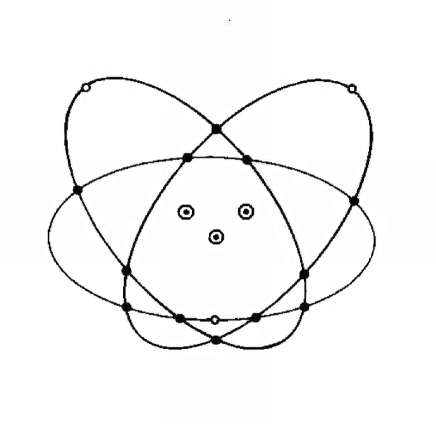
Figure 1: A schematic sketch of the structure of the projective line $PR_{\clubsuit}(1)$. Choosing any three pairwise distant points (represented by the three double circles), the remaining points of the line are all located on the neighbourhoods of the three points (three sets of points located on three different ellipses centered at the points in question). Two neighbourhoods share four points, and as there is no overlapping between the three neighbourhoods, this way we get twelve points; the existence of the remaining three points (open circles) is intimately connected with the fact that the ring $R_{\clubsuit}$ has a non-trivial Jacobson radical.

A deeper insight into the structure/properties of neighbourhoods is obtained if we consider the three canonical homomorphisms, Eqs. (8)–(10). The first two of them induce the homomorphisms from $PR_{\clubsuit}(1)$ into $PG$(1, 2), the ordinary projective line of order two, whilst the last one induces $PR_{\clubsuit}(1)\rightarrow P\widetilde{R}_{\clubsuit}(1)$. As $PG$(1, 2) consists of three points, viz. $U$: $(1,0)$, $V$: $(0,1)$ and $W$: $(1,1)$, we find that the first homomorphism, $PR_{\clubsuit}(1)\rightarrow P\widehat{R}_{\clubsuit}(1)$, acts on a neighbourhood, taken without any loss of generality to be that of $U$, as follows

$$U_{1},U_{2},U_{7},U_{8},U_{0}\rightarrow\widehat{U},$$

$$U_{5},U_{6}~{}~{}~{}~{}~{}~{}~{}~{}~{}~{}~{}~{}~{}~{}\rightarrow\widehat{V},$$ (18)

$$U_{3},U_{4}~{}~{}~{}~{}~{}~{}~{}~{}~{}~{}~{}~{}~{}~{}\rightarrow\widehat{W},$$

while the second one, $PR_{\clubsuit}(1)\rightarrow P\overline{R}_{\clubsuit}(1)$, shows an almost complementary behaviour,

$$U_{3},U_{4},U_{5},U_{6},U_{0}\rightarrow\overline{U},$$

$$U_{7},U_{8}~{}~{}~{}~{}~{}~{}~{}~{}~{}~{}~{}~{}~{}~{}\rightarrow\overline{V},$$ (19)

$$U_{1},U_{2}~{}~{}~{}~{}~{}~{}~{}~{}~{}~{}~{}~{}~{}~{}\rightarrow\overline{W}.$$

The third homomorphism, $PR_{\clubsuit}(1)\rightarrow P\widetilde{R}_{\clubsuit}(1)$, is, however, a more intricate one and in order to fully grasp its meaning we have first to understand the structure of the line $P\widetilde{R}_{\clubsuit}(1)$.

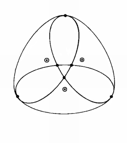
Figure 2: A schematic sketch of the structure of the projective line $P\widetilde{R}_{\clubsuit}(1)$. As in the previous case, selecting any three pairwise distant points (represented by the three double circles), the remaining points of the line (filled circles) are all located on the neighbourhoods of the three points (three sets of points located on three different ellipses centered at the points in question).

To this end in view, we shall follow the same chain of reasoning as for $PR_{\clubsuit}(1)$ and with the help of Eq. (7) and the subsequent table find that $P\widetilde{R}_{\clubsuit}(1)$ is endowed with nine points, out of which there are seven of the first kind,

$~{}~{}~{}(1,0),~{}(1,x),~{}(1,x+1),~{}(1,1),$

$~{}~{}~{}(0,1),~{}(x,1),~{}(x+1,1),$

and two of the second kind,

$~{}~{}~{}(x,x+1),~{}(x+1,x)$.

The neighbourhoods of three distinguished pairwise distant points $\widetilde{U}$: $(1,0)$, $\widetilde{V}$: $(0,1)$ and $\widetilde{W}$: $(1,1)$ here read

$$\widetilde{U}:~{}~{}\widetilde{U}_{1}:(1,x),~{}\widetilde{U}_{2}:(1,x+1),~{}\widetilde{U}_{3}:(x,x+1),~{}\widetilde{U}_{4}:(x+1,x),$$ (20)

$$\widetilde{V}:~{}~{}\widetilde{V}_{1}:(x,1),~{}\widetilde{V}_{2}:(x+1,1),~{}\widetilde{V}_{3}:(x,x+1),~{}\widetilde{V}_{4}:(x+1,x),$$ (21)

and

$$\widetilde{W}:~{}~{}\widetilde{W}_{1}:(1,x),~{}\widetilde{W}_{2}:(1,x+1),~{}\widetilde{W}_{3}:(x,1),~{}\widetilde{W}_{4}:(x+1,1).$$ (22)

From these expressions, and the fact that the coordinates of any three mutually distant points can again be made identical to those of $\widetilde{U}$, $\widetilde{V}$ and $\widetilde{W}$, we find that the neighbourhood of any point of this line comprises four distinct points, the neighbourhoods of any two distant points have two points in common (which again implies non-transitivity of the neighbour relation) and the neighbourhoods of any three mutually distant points are disjoint—as illustrated in Figure 2; note that in this case there exist no “Jacobson” points, i. e. the points belonging solely to a single neighbourhood, due to the trivial character of the Jacobson radical, ${\cal\widetilde{J}}_{\clubsuit}=\{0\}$. At this point we can already furnish an explicit expression for $PR_{\clubsuit}(1)\rightarrow P\widetilde{R}_{\clubsuit}(1)$:

$$U_{1}/W_{1},U_{2}/W_{2}\rightarrow\widetilde{U}_{1}/\widetilde{W}_{1},~{}~{}U_{3}/W_{3},U_{4}/W_{4}\rightarrow\widetilde{U}_{2}/\widetilde{W}_{2},~{}~{}U_{5}/V_{5},U_{6}/V_{6}\rightarrow\widetilde{U}_{3}/\widetilde{V}_{3},$$

$$U_{7}/V_{7},U_{8}/V_{8}\rightarrow\widetilde{U}_{4}/\widetilde{V}_{4},~{}~{}V_{1}/W_{5},V_{2}/W_{6}\rightarrow\widetilde{V}_{1}/\widetilde{W}_{3},~{}~{}V_{3}/W_{7},V_{4}/W_{8}\rightarrow\widetilde{V}_{2}/\widetilde{W}_{4},$$ (23)

$$U,U_{0}\rightarrow\widetilde{U},~{}~{}V,V_{0}\rightarrow\widetilde{V},~{}~{}W,W_{0}\rightarrow\widetilde{W}.$$

This mapping will play an especially important role in the physical applications of the theory.

5 Envisaged Applications of the Two Geometries

We assume that $P\widetilde{R}_{\clubsuit}(1)$ and $PR_{\clubsuit}(1)$ provide a suitable algebraic geometrical setting for a proper understanding of two- and three-qubit states as embodied in the structure of the so-called Peres-Mermin “magic” square and pentagram, respectively [20]. The Peres-Mermin square is made of a three-by-three square “lattice” of nine 4-dimensional operators (or matrices) with degenerate eigenvalues $\pm 1$. The three operators in every line/column are mutually commuting, and each one is the product of the two others in the same line/column, except for the last column where a minus sign appears. The algebraic rule for the eigenvalues contradicts the one for operators, which is the heart of the Kochen-Specker theorem [21] for this particular case. The explanation of this puzzling behaviour is that three lines and two columns have joint orthogonal bases of unentangled eigenstates, while the operators in the third column share a base of maximally entangled states. We will establish a one-to-one relation between the observables in the Peres-Mermin square and the points of the projective line $P\widetilde{R}_{\clubsuit}(1)$. A closely related phenomenon occurs in a three-qubit case, with the square replaced by a pentagram involving ten operators, and the geometrical explanation will here be based on the properties of the neighbourhood of a point of the projective line $PR_{\clubsuit}(1)$. These and some other closely related quantum mechanical issues will be examined in detail in Part II of the paper.


Acknowledgements

The first author thanks Dr. Milan Minarovjech for insightful remarks and suggestions, Mr. Pavol Bendík for a careful drawing of the figures and Dr. Richard Komžík for a computer-related assistance. This work was supported, in part, by the Science and Technology Assistance Agency (Slovak Republic) under the contract $\#$ APVT–51–012704, the VEGA project $\#$ 2/6070/26 (Slovak Republic) and the ECO-NET project $\#$ 12651NJ “Geometries Over Finite Rings and the Properties of Mutually Unbiased Bases” (France).

References

- [1] Törner G, Veldkamp FD. Literature on geometry over rings. J Geom 1991;42:180–200.
- [2] Saniga M, Planat M. Hjelmslev geometry of mutually unbiased bases. J Phys A: Math Gen 2006;39:435–40. Available from math-ph/0506057.
- [3] Saniga M, Planat M. Projective planes over “Galois” double numbers and a geometrical principle of complementarity. J Phys A: Math Gen 2006, submitted. Available from math.NT/0601261.
- [4] Veldkamp FD. Projective planes over rings of stable rank 2. Geom Dedicata 1981;11:285–308.
- [5] Veldkamp FD. Projective ring planes and their homomorphisms. In: Kaya R, Plaumann P, Strambach K, editors. Rings and geometry (NATO ASI). Dordrecht: Reidel; 1985. p. 289–350.
- [6] Veldkamp FD. Projective ring planes: some special cases. Rend Sem Mat Brescia 1984;7:609–15.
- [7] Veldkamp FD. Geometry over rings. In: Buekenhout F, editor. Handbook of incidence geometry. Amsterdam: Elsevier; 1995. p. 1033–84.
- [8] Hjelmslev J. Die natürliche geometrie. Abh Math Sem Univ Hamburg 1923;2:1–36.
- [9] Klingenberg W. Projektive und affine Ebenen mit Nachbarelementen. Math Z 1954;60:384–406.
- [10] Kleinfeld E. Finite Hjelmslev planes. Illinois J Math 1959;3:403–7.
- [11] Dembowski P. Finite geometries. Berlin – New York: Springer; 1968. p. 291–300.
- [12] Drake DA, Jungnickel D. Finite Hjelmslev planes and Klingenberg epimorphism. In: Kaya R, Plaumann P, Strambach K, editors. Rings and geometry (NATO ASI). Dordrecht: Reidel; 1985. p. 153–231.
- [13] Fraleigh JB. A first course in abstract algebra (5th edition). Reading (MA): Addison-Wesley; 1994. p. 273–362.
- [14] McDonald BR. Finite rings with identity. New York: Marcel Dekker; 1974.
- [15] Raghavendran R. Finite associative rings. Comp Mathematica 1969;21:195–229.
- [16] Herzer A. Chain geometries. In: Buekenhout F, editor. Handbook of incidence geometry. Amsterdam: Elsevier; 1995. p. 781–842.
- [17] Blunck A, Havlicek H. Projective representations I: Projective lines over a ring. Abh Math Sem Univ Hamburg 2000;70:287–99.
- [18] Blunck A, Havlicek H. Radical parallelism on projective lines and non-linear models of affine spaces. Mathematica Pannonica 2003;14:113–27.
- [19] Havlicek H. Divisible designs, Laguerre geometry, and beyond. A preprint available from http://www.geometrie.tuwien.ac.at/havlicek/dd-laguerre.pdf
- [20] Mermin ND. Hidden variables and two theorems of John Bell. Rev Mod Phys 1993;65(3):803–15.
- [21] Kochen S, Specker E. The problem of hidden variables in quantum mechanics. J Math Mechanics 1967;17:59–87.