Ground state approximation for strongly interacting systems in arbitrary dimension

Abstract

We introduce a variational method for the approximation of ground states of strongly interacting spin systems in arbitrary geometries and spatial dimensions. The approach is based on weighted graph states and superpositions thereof. These states allow for the efficient computation of all local observables (e. g. energy) and include states with diverging correlation length and unbounded multi-particle entanglement. As a demonstration we apply our approach to the Ising model on 1D, 2D and 3D square-lattices. We also present generalizations to higher spins and continuous-variable systems, which allows for the investigation of lattice field theories.

Strongly correlated quantum systems are of central interest in several areas of physics. Exotic materials such as high-$T_{c}$ superconductors and quantum magnets exhibit their remarkable properties due to strong quantum correlations, and experimental breakthroughs with e.g. atomic gases in optical lattices provide a perfect playground for probing strongly correlated quantum systems. The main obstacle in understanding the behavior of those quantum systems is the difficulty in simulating the effective Hamiltonians that describe their properties. In most cases, the strong correlations in the exponentially large Hilbert space render an exact solution infeasible, and attacking the problem by numerical means requires sophisticated techniques such as quantum Monte Carlo (QMC) methods or the density matrix renormalization group (DMRG) approach Wh91 ; Sc04 .

QMC methods suffer from the sign problem which makes them inappropriate for the description of fermionic and frustrated quantum systems. DMRG is a variational approach that provides approximations to ground states, thermal states and dynamics of many–body systems. Recent insight from entanglement theory have lead to an improved understanding of both the success and the limitations of this approach. Indeed, the accuracy of the method is closely linked to the amount of entanglement in the approximated states Vi03 ; Ve04 . Matrix product states FNW92 , which provide the structure underlying DMRG, are essentially one–dimensional and the entanglement entropy of these states is limited by the dimension $D$ of the matrices, which in turn is directly linked to the computational cost Vi03 ; Sc04 . Hence a successful treatment of systems with bounded entanglement, e.g. one–dimensional, non–critical spin systems with short range interactions, is possible, while the method is inefficient for systems with an unbounded amount of entanglement, e.g. critical systems and systems in two or more dimensions. Promising generalizations that can deal with higher dimensional systems have been reported recently Ve04b ; Vi05 . However, the computational effort and complexity increases with the dimension of the system. In addition, the amount of block-wise entanglement of the states used in Ref. Ve04b still scales proportional at most to the surface of a block of spins, whereas in general a scaling in proportion to the volume of the block is possible. Such a scaling can in fact be observed for disordered systems Ca05 or systems with long–range interactions Du05 .

Here we introduce a new variational method using states with intrinsic long-range entanglement and no bias towards a geometry to overcome these limitations. We first illustrate our methods for spin-1/2 systems, and then generalize them to arbitrary spins and infinite dimensional systems such as harmonic oscillators. In finite dimensions, the method is based on a certain class of multiparticle–entangled spin states, weighted graph states (WGS) and superpositions thereof. WGS are a $O(N^{2})$ parameter family of $N$–spin states with the following properties: (i) they form an (overcomplete) basis, i.e. any state can be represented as a superpositions of WGS; (ii) one can efficiently calculate expectation values of any localized observable, including energy, for any WGS; (iii) they correspond to weighted graphs which are independent of the geometry and hence adaptable to arbitrary geometries and spatial dimensions; (iv) the amount of entanglement contained in WGS may be arbitrarily high, in the sense that the entanglement between any block of $N_{A}$ particles and the remaining system may be $O(N_{A})$ and the correlation length may diverge.

Note that (iii) and (iv) are key properties in which this approach differs from DMRG and its generalizations and which suggest a potential for enhanced performance at least in certain situations, while (ii) is necessary to efficiently perform variations over this family. In the following we will outline how we use superpositions of a small number of WGS as variational ansatz states to find approximations to ground states of strongly interacting spin systems in arbitrary spatial dimension.

Properties of WGS. WGS are defined as states of $N$ spin-$1/2$ (or qubits), that result from applying phase gates $U_{ab}(\varphi_{ab})=\operatorname{diag}(1,1,1,e^{-i\varphi_{ab}})$ onto each pair of qubits $a,b\in\{1,2,\dots,N\}$ of a tensor product of $\sigma_{x}$-eigenstates $|+\rangle=(|0\rangle+|1\rangle)/\sqrt{2}$, followed by a single-qubit filtering operation $D_{a}=\operatorname{diag}(1,e^{d_{a}})$, $d_{a}\in\mathbb{C}$ and a general unitary operation $U_{a}$

$$|\Psi_{\Gamma,\mathbf{d},U}\rangle\propto\prod_{a=1}^{N}U_{a}D_{a}\prod_{b=a+1}^{N}U_{ab}(\varphi_{ab})|+\rangle^{\otimes N}.$$ (1)

The phases $\varphi_{ab}$ can be associated with a weighted graph with a real symmetric adjacency matrix $\Gamma_{ab}=\varphi_{ab}$. For convenience, we define a deformation vector $\mathbf{d}=(d_{1},d_{2},\ldots,d_{N})$ and $U\equiv{\bigotimes}_{a}U_{a}$. The deformations make WGS as used in this letter slightly more general than the WGS used in Refs. Ca05 ; Du05 where $d_{a}=0$. One can conveniently rewrite $|\Psi_{\Gamma,\mathbf{d},U}\rangle$ as

$$|\Psi_{\Gamma,\mathbf{d},U}\rangle\propto U\sum_{\bm{s}}e^{-i{\bm{s}}^{T}\Gamma{\bm{s}}/2+\mathbf{d}^{T}{\bm{s}}}|{\bm{s}}\rangle,$$ (2)

where the sum runs over all computational basis states, which are labelled with the binary vector ${\bm{s}}=(s_{1},s_{2},\ldots,s_{N})^{T}$. Our class of variation states comprises superpositions of WGS of the form

$$|\Psi\rangle\propto\sum_{i=1}^{m}\alpha_{i}|\Psi_{\Gamma,\mathbf{d}^{(i)},U}\rangle,$$ (3)

i. e. the superposed states differ only in their deformation vector $\mathbf{d}^{(i)}$, while the adjacency matrix $\Gamma$ and the unitary $U$ are fixed. Such a state is specified by $N(N-1)/2+3N+2(N+1)m=O(N^{2})$ real parameters.

We now proceed to verify the properties set out in the introduction. For property (i), observe that for any fixed $\Gamma$ and $U$, all possible combinations of $D_{a}\in\{\sigma_{z}^{(a)},\mbox{$1{\bf l}$}^{(a)}\}$ lead to an orthonormal basis (note that $\sigma_{z}^{(a)},\mbox{$1{\bf l}$}^{(a)}$ commute with $U_{ab}$). Hence any state $|\Psi\rangle$ can be written in the form Eq. (3) for sufficiently large $m\leq 2^{N}$, which shows the exhaustiveness of the description.

The relevance of employing deformations lies in the observation that only $|\Psi\rangle$ of the form of Eq. (3) permit the efficient evaluation of the expectation values of localized observables $A$, i.e. satisfy property (ii). For simplicity we restrict our attention to observables of the form

$$A=\sum_{a<b}A_{ab}+\sum_{a}A_{a},$$ (4)

where $A_{ab}$ has support on the two spins $a,b$. The method can be easily adopted to any observable that is a sum of terms with bounded support. To compute ${\rm tr}(A|\Psi\rangle\langle\Psi|)=\sum_{a<b}{\rm tr}(A_{ab}\rho_{ab})+\sum_{a}{\rm tr}(A_{a}\rho_{a})$ it is sufficient to determine the reduced density operators $\rho_{ab}$ and $\rho_{a}$.

For a single WGS ($m=1$)we obtain $\rho_{12}=(U_{1}\otimes U_{2})(\sum r_{\bm{s},\bm{t}}|{\bm{s}}\rangle\langle{\bm{t}}|)(U_{1}\otimes U_{2})^{\dagger}$ with

$$r_{\bm{s},\bm{t}}=e^{-i\gamma}\prod_{c=3}^{N}\left(1+e^{d_{c}+d_{c}^{*}-i\sum_{e=1}^{2}(s_{e}-t_{e})\Gamma_{ec}}\right)$$ (5)

and $\gamma=\sum_{a,b=1}^{2}\Gamma_{ab}(s_{a}s_{b}-t_{a}t_{b})+\sum_{a=1}^{2}(d_{a}s_{a}+d_{a}^{*}t_{a})$. This generalizes the formula for WGS without deformation obtained in Ref. Du05 . Eq. (5) demonstrates that for any WGS, the reduced density operator of two (and one) spins can be calculated with a number of operations that is linear in the system size $N$, as opposed to an exponential cost for a general state.

A straight-forward generalization of Eq. (5) allows one to calculate two–qubit reduced density matrices for superpositions of the form of Eq. (3) in time $O(m^{2}N)$. Therefore the expectation value of an observable $A$ of the form of Eq. (4) with $K$ terms requires $O(m^{2}KN)$ steps. This implies that even for Hamiltonians where all spins interact pairwise (and randomly), i.e. $K=N(N-1)/2$, the expectation value of the energy for our ansatz states can be obtained in $O(m^{2}N^{3})$ steps. For short–range interaction Hamiltonians, this reduces to $O(m^{2}N^{2})$. The total number of parameters (and memory cost) scales as $O(N^{2}+mN)$, which can be further reduced by employing symmetries.

Regarding (iii) and (iv), one can easily adopt a WGS to any given geometry by a proper choice/restriction of the adjacency matrix $\Gamma$. A state corresponding to a linear cluster state BrRa01 , for instance, will have only $\Gamma_{a,a+1}\neq 0$, while $\Gamma_{a,a+l}\neq 0$ would correspond to longer-ranged correlations. Different choices of $\varphi_{ab}$ lead to very different (entanglement) properties: For $\varphi_{ab}=|\mathbf{x}_{a}-\mathbf{x}_{b}|^{-\beta}$, where $\mathbf{x}_{a}$ denotes the spatial coordinates of spin $a$, one obtains diverging correlation length for two-point correlations, while block–wise entanglement can either be bounded or grow unboundedly, depending on the choice of $\beta$ Du05 . Similarly, more complicated geometries on lattices in higher spatial dimensions can be chosen.

Variational method. Any state of the form Eq. (3) with $m=\operatorname{poly}(N)$ permits the efficient calculation of expectation values of any two–body Hamiltonian $H$. A good approximation to the ground state is then obtained by numerical optimization of the parameters characterizing the state. Starting from random parameters, one descends to the nearest minimum using a general local minimizer (we used L-BFGS By95 ). Another approach that we found to work well is to keep all parameters fixed except for either those corresponding to (i) one local unitary $U_{a}$, (ii) one phase gate $U_{ab}(\varphi_{ab})$ or (iii) the deformation vector $d_{a}^{(j)}$ for one site $a$. In each case, the energy as a function of this subset of parameters turns out to be a quotient of quadratic forms, which can be optimized using the generalized-eigenvalue (Rayleigh) method. A similar result holds for the superposition coefficients $\alpha_{j}$. One then optimizes with respect to these subsets of parameters in turns until convergence is achieved. If one increases $m$ stepwise, one —somewhat surprisingly— does not get stuck in local minima.

A significant reduction of the number of parameters and the computational costs may be achieved by exploiting symmetries, or by adapting $\Gamma$ to reflect the geometrical situation. For instance, for systems with short range interactions and finite correlation length, one might restrict the range of the weighted graph, i.e. $\Gamma_{ab}=0$ if $|\mathbf{x}_{a}-\mathbf{x}_{b}|\geq r_{0}$. This reduces the number of parameters describing the WGS from $O(N^{2})$ to $O(N)$. For translationally invariant Hamiltonians, a better scheme is to let $\Gamma_{ab}$ depend only on $|\mathbf{x}_{a}-\mathbf{x}_{b}|$. This reduces the number of parameters to $O(N)$ as well, and it seems to hardly affect the accuracy of the ground state approximation. Hence, it allows one to reach high numbers of spins $N$ and thus to study also 2D and 3D systems of significant size. Trading accuracy for high speed one may even use a fully translation-invariant ansatz, where also $D_{a}$ and $U_{a}$ are constant and independent of $a$. In the latter case, for Hamiltonians with only nearest-neighbor interactions, the expectation value of the energy can be obtained by calculating only a single reduced density operator, and the computational cost to treat 2D [and 3D] systems of size $N=L^{2}$ [$N=L^{3}$] turns out to be of $O(L)$ rather than $O(N)$.

Demonstration. The Ising model. Our method allows us to determine, with only moderate computational cost, an upper bound on the ground state energy of a strongly interacting system of arbitrary geometry. Together with the Anderson lower bound, one can hence obtain a quite narrow interval for the ground state energy and observe qualitative features of the ground state footnoteDMRG . To illustrate our method, we have applied it to the Ising model in 1D, 2D and 3D with periodic boundary conditions, described by the Hamiltonian

$$H=-\sum_{\langle a,b\rangle}\sigma_{z}^{(a)}\sigma_{z}^{(b)}-B\sum_{a}\sigma_{x}^{(a)}$$ (6)

where $\langle a,b\rangle$ denotes nearest neighbors. For a spin chain with $N=20$, and a 2D lattice of size $4\times 4$ we compared our numerical ground state approximation with exact results (Fig. 1a). We have also performed calculations for larger 2D systems up to $14\times 14$. We note that the accuracy can be further improved by increasing $m$ (see Fig. 1b). In fact our numerical results suggest an exponential improvement with $m$. We have also tested the fully translation invariant ansatz with distance dependent phases, constant $d_{a}$ and alternating $U_{a}$ for 1D, 2D and 3D systems of size $N=30$, $N=900$ and $N=27000$ respectively (see Fig. 2). There, for lack of a refernce value for the exact ground state, we compare with the Anderson bound obtained by calculating the exact ground state energy $E_{A}$ for system size $N=15,3^{2},2^{3}$ respectively. In the 2D and especially the 3D case it is not expected that the Anderson bound is particularly tight and may lead to a significantly underestimation of the precisions achieved by our approach. The states approximated with this simple ansatz also show qualitatively essential features of the exact ground state. As an example, the maximal two-point correlation function $Q_{\rm max}^{a,a+1}$ (where the two point correlation functions are defined as $Q_{\alpha,\beta}^{a,b}=\langle\sigma_{\alpha}^{(a)}\sigma_{\beta}^{(b)}\rangle-\langle\sigma_{\alpha}^{(a)}\rangle\langle\sigma_{\beta}^{(b)}\rangle$) is plotted against the magnetic field $B$ in Fig. 2b. Strong indication for the occurrence of a phase transition can be observed: the correlations significantly increase around $B\approx 1.1,3.12,5.22$ in 1D, 2D, 3D respectively. This is in good agreement with estimates employing sophisticated power series expansions for the infinite systems or Padé approximants based on large scale numerical simulations, which expect the critical points at $B=1,3.04,5.14$ critpoint . We also remark that the approximated states show a scaling of block-wise entanglement proportional to the surface of the block, i. e. $S_{N_{A}}\approx\beta_{B}L^{{\rm dim}-1}$, where $\beta_{B}$ is some constant depending on magnetic field $B$, $N_{A}=L^{\rm dim}$ and ${\rm dim}$ is the spatial dimension. We can estimate $\beta_{B}$ and find that it significantly increases near the critical point.

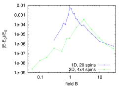
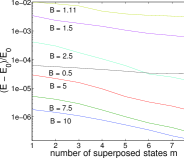
Figure 1: (Color online.) (a) Relative deviation from exact ground state energy for Ising chain with $N=20$ (blue) and $4\times 4$ 2D lattice (green) with periodic boundary conditions as function of magnetic field $B$ (calculated using BFGS minimization with symmetrized phases, $m\leq 6$). (b) 1D Ising chain with $N=20$. Improvement of relative deviation from ground state energy as function of number of superposed states $m$ for various field values $B$ (calculated using Rayleigh minimization without symmetrized phases).

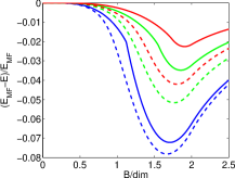
Figure 2: (Color online.) Ising model in 1D (blue) with $N=30$, 2D (green) with $N=30\times 30=900$ and 3D (red) with $N=30\times 30\times 30=27000$ spins arranged as chain, square, and cubic lattice, respectively, for fully symmetric ansatz states with $\varphi_{ab}=f(|x_{a}-x_{b}|)$, $d_{a}=1$ as function of magnetic field $B/{\rm dim}$, where ${\rm dim}$ is dimension of lattice. (a) Relative deviation of ground state energy $(E_{MF}-E)/E_{MF}$ per bond from to mean field approximation $E_{MF}$ (solid), and of Anderson bound $(E_{MF}-E_{A})/E_{MF}$ (dashed). Translational invariance is reduced by using $U_{1}\not=U_{2}$ (alternating). (b) maximal two-point correlation $Q_{\rm max}^{a,a+1}$ for nearest neighbors.

Generalizations: Our approach can be adapted directly to spin-$\frac{n}{2}$ systems using the representation Eq. (2). There the sum over binary vectors $\mathbf{s}$ with $s_{i}=0,1$ has to be changed to $n$-ary vectors $\mathbf{s}$ with $s_{i}=0,1,...,n-1$ and the corresponding matrices/vectors $\Gamma,\mathbf{d},U$ have to be modified accordingly. However, the limit $n\to\infty$ to infinite dimensional systems is both problematic and impractical, as the computational effort increases with $n$. For continuous variable systems we thus choose a closely related but slightly different approach.

The description of field theories on lattices generally leads to infinite-dimensional subsystems such as harmonic oscillators. A Klein-Gordon field on a lattice for example possesses a Hamiltonian quadratic in position and momentum operators $X$ and $P$ whose ground state is Gaussian Plenio CDE 05 . This suggests that techniques from the theory of Gaussian state entanglement (see Eisert P 03 for more details) provide the most natural setting for these problems. To this end, consider $N$ harmonic oscillators and the vector, $\mathbf{R}=(R_{1},...,R_{2N})^{T}=(X_{1},P_{1},...,X_{N},P_{N})^{T}.$ The canonical commutation relations then take the form $[R_{j},R_{k}]=i\sigma_{jk}$ with the symplectic matrix $\sigma$. All information contained in a quantum state $\rho$ can then be expressed equivalently in terms of the characteristic function $\chi_{\rho}(\bm{\xi})=\operatorname{tr}[\rho W(\bm{\xi})]$ where $\bm{\xi}\in{\mathbbm{R}}^{2N}$ and $W(\bm{\xi})=\exp(i\bm{\xi}^{T}\sigma\mathbf{R})$. Then, expectation values of polynomials of $X$ and $P$ can be obtained as derivatives of $\chi$. For Gaussian states, i.e. states whose characteristic function is a Gaussian $\chi_{\rho}(\bm{\xi})=\chi_{\rho}(0)e^{-\frac{1}{4}\bm{\xi}^{T}\gamma\bm{\xi}+\mathbf{D}^{T}\bm{\xi}}$, where here $\gamma$ is a $2N\times 2N$-matrix and $\mathbf{D}\in{\mathbbm{R}}^{2N}$ is a vector, these expectation values can be expressed efficiently as polynomials in $\gamma$ and $\mathbf{D}$. On the level of wave functions a pure Gaussian state is given by $|F,G;\mathbf{a}\rangle=C\int_{\mathbbm{R}^{N}}d^{N}xe^{-\frac{1}{2}\mathbf{x}^{T}(F-iG)\mathbf{x}+\mathbf{a}^{T}\mathbf{x}}|\mathbf{x}\rangle$ where $F$ and $G$ are real symmetric matrices, $\mathbf{a}$ is a vector, $C$ is the normalization and

$$\gamma=\left(\begin{array}[]{cc}F+GF^{-1}G&-GF^{-1}\\ -F^{-1}G&F^{-1}\end{array}\right),\;\mathbf{D}=\left(\begin{array}[]{c}GF^{-1}\mathbf{a}\\ -F^{-1}\mathbf{a}\end{array}\right).$$ (11)

Now, we may consider coherent superpositions $|\psi\rangle=\sum_{i}\alpha_{i}|G_{i},F_{i};\mathbf{a}_{i}\rangle$ to obtain refined approximations of a ground state. These do not possess a Gaussian characteristic function but a lengthy yet straightforward computation reveals that the corresponding characteristic function $\chi_{|\psi\rangle\langle\psi|}(\bm{\xi})$ is a sum of Gaussian functions with complex weights. Then it is immediately evident that in this description we retain the ability of efficient evaluation of all expectation values of polynomials in $X$ and $P$. This allows one to establish an efficient algorithm for the approximation of ground state properties of lattice Hamiltonians that are polynomial in $X$ and $P$.

Summary and Outlook: We have introduced a new variational method based on deformed weighted graph states to determine approximations to ground states of strongly interacting spin systems. The possibility to compute expectation values of local observables efficiently, together with entanglement features similar to those found in critical systems, make these states promising candidates to approximate essential features of ground states for systems with short range interactions in arbitrary geometries and spatial dimensions. One can also generalize this approach to describe the dynamics of such systems, systems with long range interactions, disordered systems, dissipative systems, systems at finite temperature and with infinite dimensional constituents. In fact, generalizations of our method that deal with these issues are possible and will be reported elsewhere.

We thank J. I. Cirac for valuable discussions and J. Eisert for suggesting the use of the Anderson bound. This work was supported by the FWF, the QIP-IRC funded by EPSRC (GR/S82176/0), the European Union (QUPRODIS, OLAQUI, SCALA, QAP), the DFG, the Leverhulme Trust (F/07 058/U), the Royal Society, and the ÖAW through project APART (W. D.). Some of the calculations have been carried using facilities of the University of Innsbruck’s Konsortium Hochleistungsrechnen.

References

- (1) S. R. White, Phys. Rev. Lett. 69, 2863 (1992); Phys. Rev. B 48, 10345 (1993).
- (2) U. Schollwöck, Rev. Mod. Phys. 77, 259 (2005).
- (3) G. Vidal, Phys. Rev. Lett. 91, 147902 (2003); 93, 040502 (2004).
- (4) F. Verstraete, D. Porras and J. I. Cirac, Phys. Rev. Lett. 93, 227205 (2004).
- (5) M. Fannes, D. Nachtergaele, and R. F. Werner, Commun. Math. Phys. 144, 443 (1992).
- (6) F. Verstraete and J. I. Cirac, e-print cond-mat/0407066.
- (7) G. Vidal, e-print cond-mat/0512165.
- (8) J. Calsamiglia et al., Phys. Rev. Lett. 95, 180502 (2005).
- (9) W. Dür, et al., Phys. Rev. Lett. 94, 097203 (2005).
- (10) H.-J. Briegel and R. Raußendorf, Phys. Rev. lett. 86, 910 (2001).
- (11) We remark that for 1D systems, the accuracies appear to scale less well in the resources as for DMRG methods. However, our approach yields accurate results also for 2D and 3D systems.
- (12) R. H. Byrd, P. Lu, and J. Nocedal, SIAM J. Sci. Stat. Comp. 16, 1190 (1995).
- (13) H.-X. He, C. J. Hamer and J. Oitmaa, J. Phys. A 23, 1775 (1990); Z. Weihong, J. Oitmaa, and C. J. Hamer, J. Phys. A 27, 5425 (1994)
- (14) K. Audenaert et al., Phys. Rev. A 66, 042327 (2002); M. B. Plenio et al., Phys. Rev. Lett. 94, 060503 (2005).
- (15) J. Eisert and M. B. Plenio, Int. J. Quant. Inf. 1, 479 (2003).