Quantum dynamics of magnetically controlled network for Bloch electrons

Abstract

We study quantum dynamics of wave packet motion of Bloch electrons in quantum networks with the tight-binding approach for different types of nearest-neighbor interactions. For various geometrical configurations, these networks can function as some optical devices, such as beam splitters and interferometers. When the Bloch electrons with the Gaussian wave packets input these devices, various quantum coherence phenomena can be observed, e.g., the perfect quantum state transfer without reflection in a Y-shaped beam, the multi- mode entanglers of electron wave by star shaped network and Bloch electron interferometer with the lattice Aharonov-Bohm effects. Behind these conceptual quantum devices are the physical mechanism that, for hopping parameters with some specific values, a connected quantum networks can be reduced into a virtual network, which is a direct sum of some irreducible subnetworks. Thus, the perfect quantum state transfer in each subnetwork in this virtual network can be regarded as a coherent beam splitting process. Analytical and numerical investigations show the controllability of wave packet motion in these quantum networks by the magnetic flux through some loops of these networks, or by adjusting the couplings on nodes. We find the essential differences in these quantum coherence effects when the different wave packets enter these quantum networks initially. With these quantum coherent features, they are expected to be used as quantum information processors for the fermion system based on the possible engineered solid state systems, such as the array of quantum dots that can be implemented experimentally.

I Introduction

Quantum information processing (QIP) has been a very active area of research in the past few years QIP1 ; QIP2 . The current challenge for QIP is to coherently integrate a sufficiently large and complex controllable system and then requires the ability to transfer quantum information between spatially separated quantum bits. Since then numerous approaches for this purpose have been proposed, ranging from linear and nonlinear quantum optical devices to various interacting quantum systems. Among them, many studies proposed using the internal dynamics of coupled spins for the transfer of quantum information QST1 ; QST2 ; QST3 ; QST4 ; QST5 ; LY ; ST ; SZ ; QST6 . However, the basic and necessary “optical devices” (for the electron wave or the spin wave) in a solid system are scarce due to the technology at hand. Therefore, it is significant to probe the possibilities to construct the artificial “optical devices” and then build the corresponding electronic networks for the matter wave of electron within a solid state system quant-network ; spin-network ; Experiment . Here, we notice that, for the boson system, Plenio, Hartley and Eisert Plenio  have studied the quantum network dynamics of a system consisting of a large number of coupled harmonic oscillators in various geometric configurations for the similar purpose.

This paper will pay attentions to the fermion systems where the Bloch electrons move along the quantum lattice network. We consider various geometrical configurations of tight-binding networks that are analogous to quantum optical devices, such as beam splitters and interferometers. We then consider the functions of these tight-binding networks in details when initially Gaussian wave packets are entering these devices. Analytical and numerical investigations show that these devices are controllable by the magnetic flux through the network. Characteristic parameters of devices can be adjusted by changing the flux or the interactions on nodes. The relevant quantum phenomena, such as generation of entanglement and the Aharonov-Bohm (AB) effects in the solid state based devices are also discussed systematically.

This paper is organized as follows. In section II, we present the Hamiltonians of the simplest tight-binding lattice systems with and without magnetic field as building blocks to construct various networks, which can be formed topologically by the linear and the various connections between the ends of them. In section III, we theoretically design and analytically study the basic properties of a star-shaped TBN, then also explore the further dynamic property of $Y$-shaped network. Surprisingly, for appropriate joint hopping integrals, the complicated network can be reduced into an imaginary linear chain with homogeneous NN hopping terms plus a smaller complicated network. It is known that such TBNs are analogous to quantum optical devices such as beam-splitters, entangler and interferometers. In section IV, we investigate the dynamic properties of a Bloch electron model on a $Q$-shaped lattice, which consists of a terminal chain and a ring threaded by a magnetic flux. The appropriate flux through the network can reduce the network to the linear virtual chain, which indicates that the flux can control the propagation of GWP in the network. In section V, the interferometer network, a mimic of the AB effect experiment, is also studied in the similar way. In addition, in the whole paper, a moving Gauss wave packet (GWP) localized in a linear dispersion regime is a good example to illustrate the properties of the above Bloch electron networks. In section VI, we extend the results of the TBNs to the spin network (SN) for the dynamics of the single magnon. In section VII, we summarize the results of this paper and suggest the possible applications of these TBNs.

II Basic setup

In this section, we introduce the systems under consideration, namely the tight-binding Bloch electron systems and the Hamiltonians of the building blocks to construct various networks. Without loss of the generality, we concentrate our attention on the simplest tight-binding systems, in which only the hopping term or kinetic energy is considered.

A general tight-binding network (TBN) is constructed topologically by the linear tight-binding chains and the various connections between the ends of them. An important element in the system is the Aharonov-Bohm flux through some loops of the TBN. Here, we consider the simplest tight-binding model, in which only the nearest neighbor (NN) hopping terms are taken into account. The Hamiltonian of a tight-binding linear chain of $N_{l}$ sites reads as

$$H_{l}=H_{l}(N_{l})\equiv-\sum_{j=1}^{N_{l}-1}(t_{j}^{[l]}a_{l,j}^{{\dagger}}a_{l,j+1}+H.c.).$$ (1)

Here, the label $l$ denotes the chain with the distribution of the hopping integrals $\{t_{1}^{[l]},t_{2}^{[l]},...,t_{N_{l}-1}^{[l]}\}$ and $a_{l,j}^{{\dagger}}$ is the fermion creation operator at $j$th site of the chain $l$. The hopping integral could be the complex number due the presence of the external magnetic field. In this paper, we restrict our study to a simplest case described as following. When the field is absent, the hopping integral for a homogeneous chain

$$t_{j}^{[l]}=te^{i\Phi_{l,j+1}}$$ (2)

in a chain is real and identical (i.e., independent of sites) while in the presence of a vector potential the hopping integral is modified by a phase factor. Here, we defined the link phase

$$\Phi_{l,j+1}=\frac{2\pi}{\phi_{0}}\int_{j}^{j+1}\mathbf{A}\cdot d\mathbf{l}$$ (3)

with flux quanta $\phi_{0}=hc/e$ as an integral of the vector potential $\mathbf{A}$ along the link between the sites $j$ and $j+1$ in the $l$th chain. The above observation about the phase modification of hopping integral can be found in many modern literatures gauge-trans ; tight-binding but the proof can be cast back to Peierls Peierls .

Another important portion of the quantum networks is the joints or nodes between two linear chains, of which the Hamiltonian can be presented in the form

$$H_{joint}\equiv-(t_{ji}^{[lm]}a_{l,j}^{{\dagger}}a_{m,i}+H.c.),$$ (4)

where $t_{ji}^{[lm]}$ denotes the hopping integral over the $j$th site of chain $l$ and the $i$th site of chain $m$. Here, only one joint term connecting two chains is listed in $H_{joint}$ as an illustration. In a general TBN, the joint Hamiltonian $H_{joint}$ should contain many connection terms.

In remaining parts of this paper, we will show that, under certain conditions, a complex TBNs can be decomposed as a simple sum of several independent imaginary chains. In order to avoid confusion, we describe one of the imaginary chains of $N_{l}$ sites by a Hamiltonian

$$\widetilde{H}_{l}=\widetilde{H}_{l}(N_{l})\equiv-t\sum_{j=1}^{N_{l}-1}(\widetilde{a}_{l,j}^{{\dagger}}\widetilde{a}_{l,j+1}+H.c.).$$ (5)

Here, $\widetilde{a}_{l,j}^{{\dagger}}$ denoted by tilde are the fermion creation operators for $j$th site of the imaginary chain $l$,  which are linear combinations of $a_{m,i}$. Namely, there exists a mapping $R$ between the two sets of fermion operators, $\{a_{l,j}^{{\dagger}}\}\overset{R}{\longrightarrow}\{\widetilde{a}_{m,i}^{{\dagger}}\}$ or by a transformation $R$:

$$\widetilde{a}_{m,i}^{{\dagger}}=\sum_{l,j}R_{l,j,m,i}a_{l,j}^{{\dagger}}$$ (6)

We will investigate several types of networks based on the notations introduced above. As an example to demonstrate the application of the notation, we can express the main conclusion of this paper by using the above well-defined notations as

$$\sum\limits_{l}H_{l}+H_{joint}\overset{R}{\longrightarrow}\sum\limits_{m}\widetilde{H}_{m},$$ (7)

i.e., a network can be equivalent to the simple sum of several independent imaginary chains with the aid of the transformation $R$.

There is a remark to be made here: In usual, the role of the potential $\mathbf{A}$ shows as the AB effect of Bloch electron in a close chain (or called a tight-binding ring). Here, the local magnetic filed strength for Bloch electron may vanish, but the loop integral of $\mathbf{A}$–the magnetic flux does not. Due to the AB effect, the magnetic flux $\phi$ can be used to control the single-particle spectrum of a homogeneous chain, $\varepsilon_{k}=-2t\cos(k+2\pi\phi/N)$. When the flux $\phi\sim\phi_{n}$ $\equiv(n/2$ $+1/4)N$, the lower spectrum becomes a linear dispersion approximately, i.e., $\varepsilon_{k}\sim k$. For the wave packets as a superposition of those eigenstates with small $k$, the linearization of Hamiltonian lead to the transfer of the wave packet without spreading YS1 .

III The basic blocks of quantum network: star- and Y-shaped beams

In this section, we use analytical method and numerical simulation to study the basic blocks of quantum network, the star- and Y-shaped beams, which is constructed by connecting one ends of several chains to the end (a node) of a single chain. Beam splitters are the elementary optical devices frequently used in classical and quantum optics QOP , which can even work well in the level of single photon quanta S-photon and are applied to generate quantum entanglement Entng . For matter wave, an early beam splitter can be referred to the experiments of neutron interference based on a perfect crystal interferometer with wavefront and amplitude division N-interfer . Moreover, for cold atoms, a beam splitter have been experimentally implemented on the atom chip C-atom . The theoretical method has been suggested to realize the beam splitter for the Bose-Einstein condensate BEC .

In the following, we begin with the basic properties of the corresponding networks for fermions. We will show that, for appropriate joint hopping integrals, the complicated network can be reduced into an imaginary linear chain with homogeneous NN hopping terms plus a smaller complicated network. We also further study the dynamic property of such kind of network by taking the $Y$-shaped network as an example of star shape beams, in which only three chains are involved. We investigate various aspects that are analogous to quantum optical devices, such as beam-splitters, entangler, and interferometers.

III.1 Star-shaped beam splitter and its reduction

Figure 1: (Color on line) (a) The star-shaped Bloch electron network with an input chain $A$ and $m$ output chains in the real space. (b) When the joint hopping constants satisfy $t_{n}=t/\sqrt{m}$, the STBN can be reduced into one homogeneous tight-binding chain $a$ with length $M+N$ and $m-1$ virtual chains with length $N$ in the virtual space.

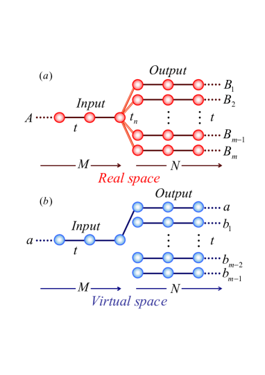
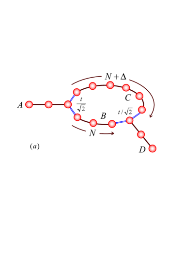
We consider a simple TBN, a star shape (we also call the star-shaped tight-binding network (STBN)) as shown in Fig. 1(a). The STBN is constructed by linking the $m$ output chains $B_{p}$ $(p=$ $1,2,$ $...,m)$ to the one end of the input chain $A$ by the hopping integrals $t_{N_{A}1}^{[AB_{p}]}$. The Hamiltonian of an STBN consists of the linear chain part (1) and the joint part (4) around the last $N_{A}$th site of the input chain $A$. Obviously, since there is no vector potential acting on the network, all the hopping integrals are real.

We will show that, under some restriction for the intrachain hopping constants $t$ and interchain hopping constants $t_{N_{A}1}^{[AB_{p}]}$, an STBN can be reduced into an imaginary linear tight-binding chain with homogeneous hopping constants plus a smaller complicated network. The fact that the input chain $A$ is a part of this virtual linear chain implies that the Bloch electron can perfectly propagate in this virtual linear chain without the reflection by the node. This also indicates that there is a coherent split of the input electronic wave because the wave function in this virtual chain actually is just a superposition of wave functions in the $m$ chains.

To sketch our central idea, we first consider a special STBN, which consists of $m$ identical “output” chains $B_{1},B_{2},\cdots,$ $B_{m}$ with homogeneous intrachain hopping constants$\ t$, interchain hopping constant$\ t_{N_{A}1}^{[AB_{p}]}=t_{n}$ and the same length $N$, while the length of chain $A$ is $M$. The Hamiltonian of the network

$$H=\sum_{p=1}^{m}H_{B_{p}}+H_{A}+H_{joint}$$ (8)

is now explicitly written in terms of the chain Hamiltonians $H_{B_{p}}$ and $H_{A}$ defined by Eq. (1). Here, the basic parameters for the network are $t_{j}^{[B_{p}]}=t_{j}^{[A]}=t$, $N_{B_{p}}=N$, and $N_{A}=M$, where $p=$ $1,2,$ $...,m$. The joint Hamiltonian is

$$H_{joint}=-t_{n}(a_{A,M}^{{\dagger}}\sum_{p=1}^{m}a_{B_{p},1}+H.c.).$$ (9)

Note that we only consider the case that all the hopping integrals over the joints are identical for the convenience of illustration. In the next section, the different joint hopping integrals will be taken into account for a simplest case of $m=2$.

Now we construct the new fermion operators denoted by the tilde notation, $\widetilde{a}_{a,j}^{{\dagger}}$ of virtual tight-binding chain $a$ of length $M+N$ as

$$\widetilde{a}_{a,j}^{{\dagger}} =a_{A,j}^{{\dagger}},$$

$$\widetilde{a}_{a,M+l}^{{\dagger}} =\frac{1}{\sqrt{m}}\sum_{p=1}^{m}a_{B_{p},l}^{{\dagger}},$$ (10)

where $j\in[1,M]$ and $l\in[1,N]$. There exist $m-1$ complementary tight-binding chains with the collective operators

$$\widetilde{a}_{b_{q},j}^{{\dagger}}=\frac{1}{\sqrt{m}}\sum_{p=1}^{m}\exp(-i2\pi pq/m)a_{B_{p},j}^{{\dagger}},$$ (11)

where $j\in[1,N]$, $p=1,2,$ $\cdots,m,$ and $q=1,2,\cdots,$ $m-1$. It can be checked that, all the tilde operators are also the standard fermion operators, which satisfy the anticommutation relation

$$\left\{\widetilde{a}_{\alpha,i},\widetilde{a}_{\beta,j}^{{\dagger}}\right\}=\delta_{\alpha\beta}\delta_{ij},$$ (12)

where $\alpha,\beta\in(a,b_{1},b_{2},\cdots,b_{m-1})$ denote the labels of the virtual chains. By inverting Eqs. (10) and (11) we have

$$a_{A,j}^{{\dagger}} =\widetilde{a}_{a,j}^{{\dagger}},\text{ }(j=1,2,\cdots,M)$$

$$a_{B_{p},j}^{{\dagger}} =\frac{1}{\sqrt{m}}\sum_{q=1}^{m-1}e^{i\frac{2\pi pq}{m}}\widetilde{a}_{b_{q},j}^{{\dagger}}+\frac{1}{\sqrt{m}}\widetilde{a}_{a,M+j}^{{\dagger}},$$

where $p\in[1,m]$, $q\in[1,m-1]$, and $j\in[1,N]$. These establish the mapping $R$ between the two sets of fermion operators, $\{a_{l,j}^{{\dagger}}\}\overset{R}{\longrightarrow}\{\widetilde{a}_{m,i}^{{\dagger}}\}$. Therefore, we have

$$H = -t\sum_{j=1}^{M-1}\widetilde{a}_{a,j}^{{\dagger}}\widetilde{a}_{a,j+1}-t\sum_{j=1}^{N-1}(\sum_{q=1}^{m-1}\widetilde{a}_{b_{q},j}^{{\dagger}}\widetilde{a}_{b_{q},j+1}$$

$$+\widetilde{a}_{a,M+j}^{{\dagger}}\widetilde{a}_{a,M+j+1})-\sqrt{m}t_{n}\widetilde{a}_{a,M}^{{\dagger}}\widetilde{a}_{a,M+1}+H.c..$$

The above Hamiltonian depicts a TBN with different geometry. It is easy to observe that only when the matching condition of the joint hopping constants

$$t_{N_{A}1}^{[AB_{p}]}=t_{n}=\frac{t}{\sqrt{m}}$$ (14)

is satisfied, we have $H=\widetilde{H}_{a}+\sum_{q=1}^{m-1}\widetilde{H}_{b_{q}}:$

$$\widetilde{H}_{a} =-t\sum_{j=1}^{M+N-1}\widetilde{a}_{a,j}^{{\dagger}}\widetilde{a}_{a,j+1}$$

$$\widetilde{H}_{b_{q}} =-t\sum_{j=1}^{N-1}\widetilde{a}_{b_{q},j}^{{\dagger}}\widetilde{a}_{b_{q},j+1}+H.c.$$ (15)

where $N_{a}=M+N$ and $N_{b_{q}}=N$. The tilde Hamiltonians are also illustrated in Fig. 1(b). Interestingly, all the sub-Hamiltonians $\widetilde{H}_{a}$, $\widetilde{H}_{b_{q}}$ commutate with each other, i.e.,

$$\left[\widetilde{H}_{\alpha},\widetilde{H}_{\beta}\right]=0,$$ (16)

where $\alpha,\beta\in(a,b_{1},b_{2},\cdots,b_{m-1})$. This fact means that the virtual chain described by $\widetilde{H}_{a}$ is just a standard tight-binding chain of length $N_{a}$ with uniform NN couplings. For an arbitrary initial state localized within the chain $H_{a}$, it will evolve driven by the virtual chain of length $M+N$. If the local state moves out of chain $H_{a}$, an ideal beam splitter can be realized since there is no reflection occurs at the node.

To demonstrate it, we take an example with the initial state as the Gaussian wave packet (GWP). The GWP with momentum $\pi/2$ has the form

$$\left|\psi(N_{0})\right\rangle=\frac{1}{\sqrt{\Omega}}\sum_{j=1}^{M}e^{-\frac{{}^{\alpha^{2}}}{2}(j-N_{0})^{2}}e^{i\frac{\pi}{2}j}\left|j\right\rangle.$$ (17)

Here, $\Omega=\sum_{j=1}^{N_{A}}\exp[-\alpha^{2}(j-N_{0})^{2}]$ is the normalization factor and $N_{0}\in[1,N_{A}]$ is the initial central position of the GWP at the input chain $A$, while the factor $\alpha$ is large enough to guarantee the locality of the state in the chain $A$. Accordingly, the basis $\left|j\right\rangle$ is defined as $\left|j\right\rangle=\widetilde{a}_{a,j}^{{\dagger}}\left|0\right\rangle$ for $j\in[1,M+N]$. In the previous work YS1 , it has been shown that such GWP can approximately propagate along a homogenous chain without spreading. Actually, at a certain time $\tau$, such GWP evolves into

$$\left|\Psi(\tau)\right\rangle = e^{-i\widetilde{H}_{a}\tau}\left|\psi(N_{0})\right\rangle\simeq\left|\psi(N_{0}+2t\tau)\right\rangle$$ (18)

$$= \frac{1}{\sqrt{\Omega}}\sum_{j=M+1}^{M+N}e^{-\frac{{}^{\alpha^{2}}}{2}(j-N_{0}-2t\tau)^{2}}e^{i\frac{\pi}{2}j}\left|j\right\rangle$$

in the virtual space. From the mapping of the operators (10), we have the final state as

$$\left|\Psi(\tau)\right\rangle=\frac{1}{\sqrt{m}}\sum_{p=1}^{m}\left|\phi_{p}(N_{\tau})\right\rangle.$$ (19)

Here, the state

$$\left|\phi_{p}(N_{\tau})\right\rangle=\frac{1}{\sqrt{\Omega}}\sum_{j=1}^{N}e^{-\frac{{}^{\alpha^{2}}}{2}(j-N_{\tau})^{2}}e^{i\frac{\pi}{2}j}a_{B_{p},j}^{{\dagger}}\left|0\right\rangle,$$ (20)

is the clone of the initial GWP with the center at $N_{\tau}=N_{0}+2t\tau-M$ in the chain $B_{p}$. Then we conclude that the beam splitter split the single-particle GWP into $m$ cloned GWPs without any reflection. Furthermore, it is obvious that the function of the splitter originates from the reduction (15) of the Hamiltonian, which is available for every invariant subspaces of fixed particle number. Therefore, such splitter can be applied to the many-particle system.

The above discussion is limited to the simplest case of identical joint hopping integrals. We would like to say that the marching condition (14) is not unique for constructing independent virtual chain. We will demonstrate this for the case $m=2$ in the next section.

III.2 Y-shaped beam splitter

Figure 2: (Color on line) (a) $Y$-shaped TBN or called $Y$-beam, a special STBN with different joint hopping integrals $t_{nB}$ and $t_{nC}$. (b) Reduction of $Y$-shaped TBN under the matching condition. It shows that if $t_{nB}^{2}+t_{nC}^{2}=t^{2}$, the $Y$-shaped TBN in real space is mapped into virtual space as two decoupled virtual chain $a$ and $b$ with length $M+N$ and $N$ respectively.

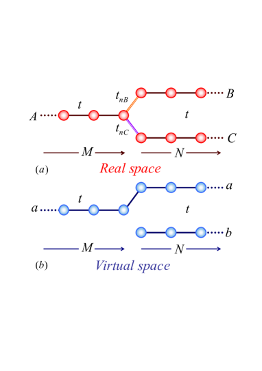
The reduction for star-shaped network was demonstrated under the restriction (14). This kind of reduction can be also performed with different joint hopping integrals. If the splitter is applied to the local GWP, the node interactions of the two output legs are not necessary to be identical. In the following, we will investigate this issue by considering the simplest configuration with $m=2$, which is called $Y$-beam. The asymmetric $Y$-beam consists of three legs $A$, $B$ and $C$ with the intrachain hopping integrals $t$ for $F=A,B,C$ and the joint ones $t_{nF}$ for $F=B,C$ (see Fig. 2(a)). The total Hamiltonian reads

$$H=\sum_{F=A,B,C}H_{F}-\sum_{F=B,C}(t_{nF}a_{A,M}^{{\dagger}}a_{F,1}+H.c.)$$ (21)

where $t_{j}^{[A]}=t_{j}^{[B]}$ $=t_{j}^{[C]}=t$, $N_{A}=M,$ and $N_{B}=N_{C}=N$.

In order to decouple this $Y$-beam as two virtual linear tight-binding chains, we need to optimize the asymmetric couplings so that the perfect transmission can occur in the decoupled linear tight-binding chains. For this purpose, we introduce the tilde operators of fermion

$$\widetilde{a}_{a,j}^{{\dagger}} =a_{A,j}^{{\dagger}},$$

$$\widetilde{a}_{a,M+l}^{{\dagger}} =\cos\theta a_{B,l}^{{\dagger}}+\sin\theta a_{C,l}^{{\dagger}},$$

$$\widetilde{a}_{b,m}^{{\dagger}} =\sin\theta a_{B,m}^{{\dagger}}-\cos\theta a_{C,m}^{{\dagger}},$$ (22)

where $j\in[1,M]$, $l\in[1,N]$, and $m\in[1,N]$. Here, the mixing angle $\theta$ is to be determined as follows by the optimization for quantum state transmission. In comparison with the optical beam splitter, the above equations (22) can be regarded as a fundamental issue for the electronic wave beam splitter.

Figure 3: (Color on line) (a) The contour map of the reflection factor $R(t_{nC},t_{nB})$ as a function of $t_{nC},t_{nB}$ for the GWP with $\alpha=0.3$ and momentum $\pi/2$ in a finite system with $N_{A}=$$N_{B}=$$N_{C}=50$. It shows that around the matching condition, i.e, the circle $t_{nC}^{2}+t_{nB}^{2}=t^{2}$, the reflection factor approaches zero. (b) The profile of $R(t_{nC},t_{nB})$ along $t_{nC}=t_{nB}$.

Together with the original creation operator $\widetilde{a}_{a,j}^{{\dagger}}=a_{A,j}^{{\dagger}}$ for the input leg, the set $\{\widetilde{a}_{a,M+j}^{{\dagger}}\mid j\in[1,N]\}$ defines a new linear chain $a$ with the effective hopping integrals

$$t_{aj} = t_{a,M+l}=t,$$

$$t_{aM} = t_{nB}\cos\theta+t_{nC}\sin\theta,$$ (23)

where $j\in[1,M-1]$ and $l\in[1,N-1]$. Another virtual linear chain $b$ is defined by $\widetilde{a}_{b,j}^{{\dagger}}$ with homogeneous hopping integral $t_{bj}=t$,$\ j\in[1,N-1]$.

In general, these two linear chains are dependent, since there is a connection interaction around the node

$$H_{joint}=-t_{AB}(\widetilde{a}_{a,M}^{{\dagger}}\widetilde{a}_{b,1}+H.c.)$$ (24)

where

$$t_{AB}=t_{nB}\sin\theta-t_{nC}\cos\theta.$$ (25)

Fortunately, the two virtual chains decouple with each other when the mixing angle $\theta$ and the intrachain connections are optimized by setting $\tan\theta=t_{nC}/t_{nB}$. And if we take $t_{AB}=t$, the virtual chain $a$ becomes a completely homogeneous chain of length $M+N$ as illustrated in Fig. 2(b). Thus, these lead to the matching condition

$$\sqrt{t_{nC}^{2}+t_{nB}^{2}}=t$$ (26)

for $Y$-beam network. It can be employed to transfer the quantum state without reflection on the node in the transformed picture. Transforming back to the original picture, we can see that such network behaves as a perfect beam splitter.

In the point of view of linear optics, such beam splitting process can generate the mode entanglement between the separated waves in chains $B$ and $C$, and the measure of such mode entanglement is determined by the values of $t_{nB}$ and $t_{nC}$. We will show that the strength of $t_{nB}$ and $t_{nC}$ can be used to control the amplitudes of the evolving Bloch electron wave packets on legs $B$ and $C$.

Now we apply the beam splitter to a special Bloch electron wave packet, a GWP with momentum $\pi/2$, which has the form (17) at $\tau=0$. It is known from the previous work YS1 that such GWP can approximately propagate along a homogenous chain without spreading. Then at a certain time $\tau$, such GWP evolves into

$$\left|\Psi(\tau)\right\rangle=\cos\theta\left|\psi_{B}(N_{\tau})\right\rangle+\sin\theta\left|\psi_{C}(N_{\tau})\right\rangle$$ (27)

where

$$N_{\tau}=N_{0}+2t\tau-M,$$ (28)

i.e., the beam splitter can split the GWP into two cloned GWPs completely. The possibility of GWPs in the arms $B$ and $C$ is determined by the mixed angle $\theta$.

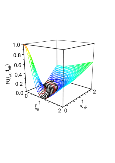
In order to verify the above analysis, a numerical simulation is performed for a GWP with $\alpha=0.3$ in a finite system with $N_{A}=N_{B}$ $=$$N_{C}=50$. Let $\left|\Phi(0)\right\rangle$ be a normalized initial state. Then the reflection factor at time $\tau$ can be defined as

$$R(t_{nC},t_{nB},\tau)=\sum_{j_{A}=1}^{M-1}\left|\left\langle j_{A}\right|e^{-iH\tau}\left|\Phi(0)\right\rangle\right|^{2}$$ (29)

to depict the reflection at the node. At an appropriate instant $\tau_{0}$,

$$R(t_{nC},t_{nB})=R(t_{nC},t_{nB},\tau_{0})$$ (30)

as a function of $t_{nC}$ and $t_{nB}$ is plotted in Fig. 3. It shows that around the matching condition (26), the reflection factor vanishes, which is just in agreement with our analytical result.

The conclusion for such GWP comes from the reduction of the $Y$-shaped network, which the equal length of two output arms is crucial. However, for the local wave packet (17), the local environment around the wave packet only result in its behavior at the next instant. This can be seen from the speed of the GWP (17). According to the study in Ref. YS1 , the speed of the GWP is independent of the size and the boundary condition (ring or open chain). Therefore, for a splitter to GWP, the equality of two output arms is not necessary. This argument will be demonstrated in the following content about quantum interferometer.

Figure 4: (Color on line) (a) The contour map of maximal concurrence of two GWPs at two legs $A$ and $B,$ $C_{\max}(t_{nC},t_{nB})$ for the same setup as that in Fig. 3. It is found that two GWPs yield the maximal entanglement at the point $t_{nC}=$$t_{nB}=$$t_{A}/\sqrt{2}$. (b) The profile of $C_{\max}(t_{nC},t_{nB})$ along $t_{nC}=t_{nB}$.

III.3 Entangler of Bloch electron

Now we consider how the STBN can behave as an entangler to produce entanglement with the $Y$-beam as an illustration. Let the input state $|\phi(0)\rangle$, represents single-particle state located in the arm $A$. It can propagate into the arms $B$ and $C$ through the node with some reflection. On the other hand, the electronic wave can be regarded as being transferred along the virtual legs $a$ and $b$. Once we manipulate the joint hopping integrals to satisfy the matching condition, the electronic wave can only enter the virtual chain $a$ rather than $b$ without any reflection. Then the final state is in the subspace of the virtual chain $a$. Similar to optical splitter, such $Y$-beam splitting can also be regarded as an entangler of fermion. For instance, consider a state $|D(j)\rangle=\widetilde{a}_{a,j}^{{\dagger}}|0\rangle$ for $j\in[M,M+N]$, which is a local state in the view of point of the virtual chain $a$. However, in the real space, this state is nonlocal and possesses mode entanglement, while state $|D(j)\rangle$ for $j\in$ $[1,M]$ is still a non-entangled state. Obviously, the $Y$-beam acts as an entangler similar to that in quantum optical systems.

To quantitatively characterize mode entanglement generated by the splitter on the joint hopping integrals $t_{nC}$, $t_{nB}$, we consider the GWP (17) as an initial state. Through the splitter, two separated GWPs are obtained. The total concurrence with respect to the two waves located at the arms $B$ and $C$ can be calculated as

$$C(\tau)=\sum_{j=1}^{N}\left|\left\langle\Psi(\tau)\right|(a_{B,j}^{{\dagger}}a_{C,j}+a_{B,j}a_{C,j}^{{\dagger}})\left|\Psi(\tau)\right\rangle\right|$$ (31)

according to refs.wang ; qian . When the interchain connections are optimized by setting $t_{nB}=t\cos\theta$, $t_{nc}=t\sin\theta$, the above mode concurrence can be calculated as

$$C(\tau)=\sin(2\theta)$$ (32)

from the Eq. (27).

It is obvious that if $\cos\theta=$ $\sin\theta=1/\sqrt{2}$, i.e.,

$$t_{nB}=t_{nC}=\frac{t}{\sqrt{2}},$$ (33)

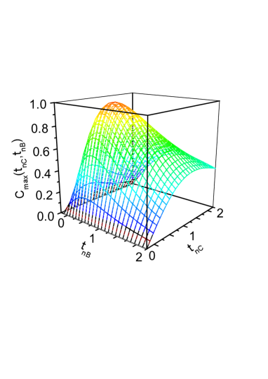
$C(\tau)$ reaches its maximum value $1$. Numerical simulation for $t_{nB},t_{nC}\in[0,2t]$ is performed for a GWP with $\alpha=0.3$ and momentum $\pi/2$ in a finite system with $N_{A}=50,$ $N_{B}=50,$ and $N_{C}=50$. The concurrence is also the function of time $\tau$ due to the dynamics of the system. We choose maximal concurrence

$$C_{\max}(t_{nC},t_{nB})=\max\{C(\tau)\}$$ (34)

as a function of $t_{nC}$ and $t_{nB}$ to depict the property of the splitter. Numerical result is plotted in Fig. 4. It shows that two split wave packets yield the maximal entanglement just at the matching point (33).

III.4 Quantum interferometer for Bloch electron

Now we consider in details a more complicated TBN than the $Y$-beam, the quantum interferometer for Bloch electron wave. This setup consists of two $Y$-beams, which is illustrated schematically in Fig. 5(a). It is similar to the optical interferometer, where state $\left|a\right\rangle$ of a single photon is split into two parts $\left|b\right\rangle$ and $\left|c\right\rangle$ by the splitter and then a new state $\left|d\right\rangle=U_{B}\left|b\right\rangle+U_{C}\left|c\right\rangle$ can be achieved by the unitary transformations $U_{B}$ and $U_{C}$. In the tight-binding Bloch electron interferometer, the analogue of the import state $\left|a\right\rangle$ is the moving GWP (17).

Figure 5: (Color on line) (a) The interferometric network with an input chain $A$ and output chain $D$, which consists of two $Y$-beams. $\Delta$ is the “optical path difference” which determines the interference pattern of output spin wave. (b) The interference pattern of output wave in the leg $D$ ($r_{0}=50$, $t_{0}=100/J_{A}$) for the GWP with $\alpha=0.3$ in the interferometric network with $N_{A}=N_{B}$ $=N_{D}=50$, $N_{C}=N_{B}+\Delta$.

Firstly, we consider the simplest case with the path difference (defined in Fig. 5(a)) $\Delta=0$. It is shown that such network is equivalent to two independent virtual chains with lengths $N_{A}+N_{B}+N_{D}$ and $N_{B}$ respectively when the coupling matching condition is satisfied. Then the initial GWP will be transmitted into the arm $D$ without any reflection. This fact can be understood according to the interference of two split GWPs. Actually, from the above analysis about the GWP propagating in the $Y$-beam, we note that the conclusion can be extended to the $Y$-beam consisting of two different length arms $N_{B}\neq N_{C}$. It is due to the locality of the GWP and the fact that the speed of the GWP only depends on the hopping integral. Then the arrival time of the two split GWPs at arm $D$ depends on the lengths $N_{B}\$and $N_{C}$. It means that the nonzero $\Delta$ should affect the shape of the pattern of output wave.

To verify the analysis above, we investigate this problem again numerically. According to quantum mechanics, the interference pattern at site $r_{0}$ and time $\tau_{0}$ in arm $D$ can be presented as

$$I(r_{0},\tau_{0},\Delta)=\left|\left\langle r_{0}\right|\exp(-iH\tau_{0})\left|\Phi(0)\right\rangle\right|^{2}.$$ (35)

Numerical simulation of $I(r_{0},\tau_{0},\Delta)$ for the input GWP in the interferometric network with $N_{A}=N_{B}$ $=N_{D}=50$, $N_{C}=N_{B}+\Delta$ is performed. For $r_{0}=50$, $\tau_{0}=100/t$, a perfect interference phenomenon by $I(r_{0},\tau_{0},\Delta)$ is observed for the range $\Delta\in[-25,25]$ in Fig. 5(b). This observation shows that the quantum interferometer can be realized by the TBN.

IV $Q$-shaped TBN controlled by flux

From the above discussion, it can be found that the essence of the reduction for the TBN lies on the interference of the matter wave. On the other hand, the presence of vector potential can induce a phase factor to the wave function and then the magnetic flux can control the coherent reduction to some extent. In this section, we investigate how to control the motion of the Bloch electron along this TBN by an external magnetic field. We will show that the appropriate flux through the network can reduce the network to the linear virtual chain, which indicate that the flux can control the propagation of GWP in the network.

IV.1 Model and Hamiltonian

Consider a quantum network constructed by connecting the two free ends of the two identical chains in $Y$-beam. Such a network is called $Q$-shaped TBN, or QTBN labelled by $\{A,B,C\}$. As illustrated schematically in Fig. 6(a), QTBN is placed in an external magnetic field. The ring of the model is threaded by a magnetic flux $\phi$ in the unit of flux quanta. Here, we only consider effect of the vector potential $\mathbf{A}$ without the Zeeman term for simply. The Hamiltonian of our $Q$-shaped lattice model reads

$$H=H_{A}+H_{B}+H_{C}+H_{joint}$$ (36)

where

$$H_{joint} = -(t_{nB}a_{A,M}^{{\dagger}}a_{B,1}e^{i\Phi_{B,1}}+t_{nC}a_{A,M}^{{\dagger}}a_{C,1}e^{-i\Phi_{C,1}})$$ (37)

$$-ta_{B,N}^{{\dagger}}a_{C,N}e^{i\Phi_{BC}}+H.c.$$

and the parameters $N_{A}=M$, $N_{B}=N_{C}=N$, $t_{j}^{[A]}=t$, $t_{j}^{[B]}=t\exp(i\Phi_{B,j+1})$, $t_{j}^{[C]}=t\exp(-i\Phi_{C,j+1})$. Here, $\Phi_{B,l}$, $\Phi_{C,l}$, $l\in[1,,N]$ denote the phase differences between the neighboring sites $l$ and $l+1$ in the chains $B$ and $C$, while $\Phi_{BC}$ is respect to the connection between the two chain. The values of the phase difference is defined as (3) and $\Phi_{B,l}$, $\Phi_{C,l}$, and $\Phi_{BC}$ are not required to be identical in order to avoid losing generality.

In the following discussion, what we concern is only the sum of the phase difference along the loop

$$\Phi=\sum_{l=1}^{N}(\Phi_{B,l}+\Phi_{C,l})+\Phi_{BC}$$ (38)

corresponding to the flux $\phi=\Phi/2\pi$ through the loop. We will show that the flux $\phi$ can control the dynamics of the $Q$-shaped lattice system.

IV.2 Reduction of the $Q$-shaped lattice model

The QTBN with the flux $\phi$, and the joint hopping strengths $t_{nB}$, $t_{nC}$, exhibits a rich variety of dynamic behaviors. Fortunately, we find that there exist analytical results in some range of parameters. Together with the numerical simulation, these analytical results are helpful to get a comprehensive understanding of the mechanism. We start with the cases of fixed $\Phi$ but various $t_{nB}$, $t_{nC}$ and then investigate the cases, vice versa.

Figure 6: (Color on line) (a) The $Q$-shaped Bloch electron network with an input chain $A$ and a ring ${B,C}$ threaded by a magnetic flux. (b) When $\phi=n/2$ and $t_{nB}=t_{nC}=t/\sqrt{2}$, the $Q$-shaped Bloch electron network can be decoupled into two virtual homogeneous linear chains $a$ and $b$ with length $M+N$ and $N$ respectively. (c) When $\phi=n/2+1/4$ and $t_{nB}^{2}+t_{nC}^{2}=t^{2}$, the $Q$-shaped Bloch electron network can be decoupled into a long virtual homogeneous linear chain $a$ with length $M+2N$. (d) If $t_{nB}=t_{nC}=t/\sqrt{2}$, as to an arbitrary $\phi$, the virtual homogeneous linear chains $a$ and $b$ are connected by the hopping integral $\widetilde{t}$. There also exist chemical potentials $-\mu$ and $\mu$ at the ends of the virtual chains $a$ and $b$ respectively.

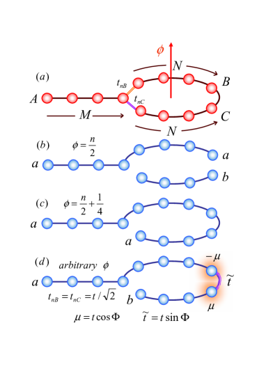
IV.2.1 Case: $\phi=\frac{n}{2}$

Our aim is try to decouple this $Q$-shaped model as two virtual linear chains. We first introduce two anticommutative sets of fermion operator $\{\widetilde{a}_{a,M+j}^{{\dagger}}\}$, $\{\widetilde{a}_{b,j}^{{\dagger}}\}$ defined by

$$\widetilde{a}_{a,M+j}^{{\dagger}} = \cos\theta e^{-i\varphi_{B}^{j}}a_{B,j}^{{\dagger}}+\sin\theta e^{i\varphi_{C}^{j}}a_{C,j}^{{\dagger}}$$

$$\widetilde{a}_{b,j}^{{\dagger}} = \sin\theta e^{-i\varphi_{B}^{j}}a_{B,j}^{{\dagger}}-\cos\theta e^{i\varphi_{C}^{j}}a_{C,j}^{{\dagger}}$$ (39)

for $j\in[1,N]$, where $\varphi_{\alpha}^{j}=\sum_{l=1}^{j}\Phi_{\alpha,l}$, $(\alpha=B,C)$.

We can check that they still satisfy the anticommutation relations $\{\widetilde{a}_{\alpha,i},\widetilde{a}_{\beta,j}^{{\dagger}}\}=\delta_{\alpha\beta}\delta_{ij}$, where $\alpha,\beta\in(a,b)$. The inverse transformations of Eq. (39), together with the original fermion operator $\widetilde{a}_{a,j}^{{\dagger}}=a_{A,j}^{{\dagger}},$ $j\in[1,M]$, define a new linear chain $a$, while another virtual linear chain $b$ is only constructed by $\widetilde{a}_{b,j}^{{\dagger}}$, $j\in[1,N]$. Therefore, the parameters are taken as

$$\phi=\frac{n}{2};t_{nB}=t_{nC}=\frac{t}{\sqrt{2}},$$ (40)

the Hamiltonian can be reduced as

$$H = \widetilde{H}_{a}+\widetilde{H}_{b}+\widetilde{H}_{\mu}$$

$$\widetilde{H}_{\mu} = t(-1)^{n}\widetilde{n}_{a,M+N}-t(-1)^{n}\widetilde{n}_{b,N}$$ (41)

with $N_{a}=M+N$ and $N_{b}=N$. Here, $\widetilde{n}_{a,M+N}=\widetilde{a}_{a,M+N}^{{\dagger}}\widetilde{a}_{a,M+N}$ and $\widetilde{n}_{b,N}=\widetilde{a}_{b,N}^{{\dagger}}\widetilde{a}_{b,N}$ are the particle number operators. The $\widetilde{H}_{\mu}$ represents the chemical potential at the ends of chains $a$ and $b$. For large $N$ system, the effect of the end potentials can be ignored. Thus the $Q$-type lattice can be reduced into two independent virtual linear chains $a$ and $b$ with homogeneous NN hopping integrals, and length $M+N$ and $N$ respectively as illustrated in Fig. 6(b).

IV.2.2 Case: $\phi=\frac{n}{2}+\frac{1}{4}$

In this case, we will show that the model can be reduced to a virtual chain with $M+2N$ sites if the joint hopping integrals satisfy $\sqrt{t_{nC}^{2}+t_{nB}^{2}}=t$. We introduce the fermion operators

$$\widetilde{a}_{a,j}^{{\dagger}} = a_{A,j}^{{\dagger}},$$

$$\widetilde{a}_{a,M+l}^{{\dagger}} = \cos\theta e^{-i\varphi_{B}^{l}}a_{B,l}^{{\dagger}}+\sin\theta e^{i\varphi_{C}^{l}}a_{C,l}^{{\dagger}},$$

$$\widetilde{a}_{a,M+N+l}^{{\dagger}} = i(-1)^{n}[\sin\theta e^{-i\varphi_{B}^{l}}a_{B,l}^{{\dagger}}-\cos\theta e^{i\varphi_{C}^{l}}a_{C,l}^{{\dagger}}],$$

where $\ j\in[1,M]$, $l\in[1,N]$. Similarly, when we set

$$\phi=\frac{n}{2}+\frac{1}{4};t_{nB}=t\cos\theta,t_{nC}=t\sin\theta$$ (43)

the Hamiltonian becomes

$$H=\widetilde{H}_{a},$$ (44)

with $N_{a}=M+2N,$ which is illustrated schematically in Fig. 6(c). Then we conclude that, when the flux is $\phi=n/2+1/4$ and the joint hopping integrals satisfy $\sqrt{t_{nC}^{2}+t_{nB}^{2}}=t$, the QTBN is equivalent to a single virtual open chain $a$ with length $M+2N$.

IV.2.3 Case: arbitrary $\phi,$ $t_{nB}=t_{nC}=\frac{t}{\sqrt{2}}$

When we take the interchain hopping integrals as $t_{nB}=t_{nC}=t/\sqrt{2}$, the mapping (39) reduces the network Hamiltonian as

$$H = \widetilde{H}_{a}+\widetilde{H}_{b}+\widetilde{H}_{ab},$$

$$\widetilde{H}_{ab} = -\mu(\widetilde{a}_{a,M+N}^{{\dagger}}\widetilde{a}_{a,M+N}-\widetilde{a}_{b,N}^{{\dagger}}\widetilde{a}_{b,N})$$ (45)

$$-\widetilde{t}(\widetilde{a}_{b,N}^{{\dagger}}\widetilde{a}_{a,M+N}+H.c.).$$

with $N_{a}=M+N$, $N_{b}=N$. We have replaced $i\widetilde{a}_{b,N}^{{\dagger}}$ by $\widetilde{a}_{b,N}^{{\dagger}}$ for $j\in[1,N]$ without influence on the physics of dynamical process. Here, $\widetilde{H}_{a}$ and $\widetilde{H}_{b}$ stand for two virtual chains with length $M+N$ and $N$ respectively, $\widetilde{H}_{ab}$ represents the chemical potential at the ends of chains $a$ and $b$ and the connection between the two sites. Note that the end-site chemical potentials possess the same magnitude $\mu=t\cos\Phi$, but of opposite sign and the hopping integral between the two end sites is $\widetilde{t}=t\sin\Phi$. The reduced model is also illustrated in Fig. 6(d).

Physically, the chemical potentials $\mu$ and the hopping integral $\widetilde{t}\$have the complementary relation $\mu^{2}+\widetilde{t}^{2}=t^{2}$. When $\Phi=(n+1/2)\pi$, the network is equivalent to a linear chain with length $M+2N$; while for $\Phi=n\pi$ it corresponds to two independent chains with lengths $M+N$ and $N$. In the next section, we will focus on such system for arbitrary $\Phi$. We will show that such system behaves as an optical device, a transmission-reflection film, while the flux determines the coefficient. In conclusion, the magnetic flux $\phi$ can influence the “effective length” or the connective status of the virtual chains and then can be used to control the dynamics of the network.

IV.3 Transmission-reflection film

Figure 7: (Color on line) (a) Schematic illustration for the transmission-reflection film in real space. Two terminal sites of the two TBNs $\{A,B\}$ are connected by the hopping integral $\widetilde{t}=t\sin\Phi$. There also exist chemical potentials $\mu=-t\cos\Phi$ for the terminal site of chain $A$ and $\mu=t\cos\Phi$ for the one of chain $B$. (b) The above TBN can be recomposed as a homogeneous chain $\{a,b\}$ in virtual space.

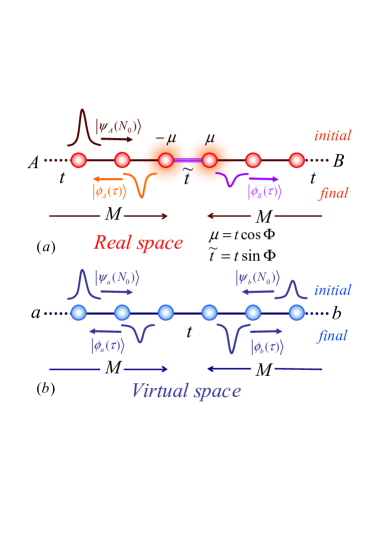
To make the above observation more clear, we consider two identical tight-binding chains $\{A,B\}$, which consist of $N$ sites respectively. There exists a connection interaction between the two terminal sites of the two virtual chains. The hopping constant is $t\sin\Phi$ and each terminal site also has a chemical potential, $\pm t\cos\Phi$. The Hamiltonian reads

$$H=H_{A}+H_{B}+H_{joint}$$ (46)

where $N_{A}=N_{B}=N$, $t_{j}^{[A]}=t_{j}^{[B]}=t$, and

$$H_{joint} = -t\sin\Phi(a_{A,N}^{{\dagger}}a_{B,N}+H.c.)$$

$$-t\cos\Phi a_{A,N}^{{\dagger}}a_{A,N}+t\cos\Phi a_{B,N}^{{\dagger}}a_{B,N}.$$

Obviously, it is the simplest case of the system described by Eq. (IV.2.3).

In order to study the properties of this Bloch electron model more clearly, we introduce two anticommutative sets of fermion operators

$$\widetilde{a}_{a,j}^{{\dagger}} = \frac{\sqrt{2}}{2}\left(f_{+}a_{A,j}^{{\dagger}}-f_{-}a_{B,j}^{{\dagger}}\right)$$

$$\widetilde{a}_{b,j}^{{\dagger}} = \frac{\sqrt{2}}{2}\left(f_{-}a_{A,j}^{{\dagger}}+f_{+}a_{B,j}^{{\dagger}}\right)$$ (48)

where $j\in[1,N]$ and

$$f_{\pm}=\cos\frac{\Phi}{2}\pm\sin\frac{\Phi}{2}.$$ (49)

The inverse transformation of Eq. (48) results in the reduction of the network described by

$$H=\widetilde{H}_{a}+\widetilde{H}_{b}+\widetilde{H}_{joint}$$ (50)

where $N_{a}=N_{b}=N$, and

$$\widetilde{H}_{joint}=-t(\widetilde{a}_{a,N}^{{\dagger}}\widetilde{a}_{b,N}+H.c.).$$ (51)

Obviously, the Hamiltonian (50) depicts an imaginary linear chain with homogeneous couplings $t$ no matter how much the magnitude of the flux $\Phi$ is taken. Then, the Hamiltonian describing transmission-reflection is mapped into a chain in virtual space. Interestingly, such mapping is irrelevant to the state concerned.

In order to demonstrate the function of such network, we study the propagation of a moving GWP. To this end, we consider a GWP defined as (17) at chain $A$, i.e.,

$$\left|\psi_{A}(N_{0})\right\rangle=\frac{1}{\sqrt{\Omega_{1}}}\sum_{j=1}^{N}e^{-\frac{\alpha^{2}}{2}(j-N_{0})^{2}}e^{i\frac{\pi}{2}j}a_{A,j}^{{\dagger}}\left|0\right\rangle.$$ (52)

We require this wave packet to satisfy $\left\langle 0\right|a_{B,j}\left|\psi_{A}(N_{0})\right\rangle\simeq 0$, so that it ensures the initial GWP being located in chain $A$. The transformation (48) means that such GWP corresponds to the combination of two GWPs in virtual space with the centers at $N_{0}$ respectively,

$$\left|\psi_{a(b)}(N_{0})\right\rangle=\frac{f_{+(-)}}{\sqrt{2\Omega_{1}}}\sum_{j=1}^{N}e^{-\frac{\alpha^{2}}{2}(j-N_{0})^{2}}e^{i\frac{\pi}{2}j}a_{a(b),j}^{{\dagger}}\left|0\right\rangle.$$ (53)

Based on the analytical result in Ref. YS1 , the two GWPs in the virtual chain should travel along the chain defined by Eq. (50) without spreading as time evolution. Then, at a certain time $\tau$, the evolved state $\left|\phi_{a(b)}(\tau)\right\rangle=$ $\exp(-i\widetilde{H}\tau)\left|\psi_{a(b)}(N_{0})\right\rangle$, or

$$\left|\phi_{a(b)}(\tau)\right\rangle = \frac{1}{\sqrt{2\Omega_{1}}}[f_{+(-)}\sum_{j=1}^{N}e^{-\frac{\alpha^{2}}{2}(j-N_{\tau})^{2}}e^{i\frac{\pi}{2}j}$$

$$+f_{-(+)}\sum_{j=1}^{N}e^{-\frac{\alpha^{2}}{2}(Pj-N_{\tau})^{2}}e^{i\frac{\pi}{2}Pj}]a_{a(b),j}^{{\dagger}}\left|0\right\rangle$$

describes the superposition of two GWPs. Here, $Pj=2N+1-j,$ $N_{\tau}=N_{0}+2t\tau$.

Transforming back to the real space, we rewrite the time evolution by the state

$$\left|\Psi(\tau)\right\rangle=\cos\Phi\left|\phi_{A}(\tau)\right\rangle+\sin\left|\phi_{B}(\tau)\right\rangle$$ (55)

in terms of the two components of the wave function

$$\left|\phi_{A}(\tau)\right\rangle = \frac{1}{\sqrt{\Omega_{1}}}\sum_{j=1}^{N}[e^{-\frac{\alpha^{2}}{2}(Pj-N_{\tau})^{2}}e^{i\frac{\pi}{2}Pj}$$

$$+\frac{1}{\cos\Phi}e^{-\frac{\alpha^{2}}{2}(j-N_{\tau})^{2}}e^{i\frac{\pi}{2}j}]a_{A,j}^{{\dagger}}\left|0\right\rangle$$

$$\approx \frac{1}{\sqrt{\Omega_{1}}}\sum_{j=1}^{N}e^{-\frac{\alpha^{2}}{2}(Pj-N_{\tau})^{2}}e^{i\frac{\pi}{2}Pj}a_{A,j}^{{\dagger}}\left|0\right\rangle$$

and

$$\left|\phi_{B}(\tau)\right\rangle=\frac{1}{\sqrt{\Omega_{1}}}\sum_{j=1}^{N}e^{-\frac{\alpha^{2}}{2}(Pj-N_{\tau})^{2}}e^{i\frac{\pi}{2}Pj}a_{B,j}^{{\dagger}}\left|0\right\rangle.$$ (57)

Here, in Eq. (LABEL:phia), the second term is ignored in the case $\left|j-N_{\tau}\right|\gg 1$.

Obviously, the central positions of the final sub-GWPs $2N+1-N_{\tau}$ decrease with time $\tau$. This observation indicates that, the beam splitter can split the GWP into two cloned GWPs with opposite moving directions along with $AB$ chain. Therefore, state $\left|\phi_{A}(\tau)\right\rangle$ represents the reflection component with probability $\cos^{2}\Phi$, while state $\left|\phi_{B}(\tau)\right\rangle$ is the transmission component through the connection of $AB$ with probability $\sin^{2}\Phi$. So this Bloch electron network for a moving GWP behaves like an optical transmission-reflection film for photons. Interestingly, transmission and reflection coefficients are governed by the parameter $\Phi$, the flux through the network. This feature is illustrated in Fig. 7 in details.

IV.4 The dynamic properties of the $Q$-shaped Bloch electron model

Now we take the propagation of the GWP $\left|\psi_{A}(N_{0})\right\rangle$ as an example. Its advantage is that the GWP we often used can move along a homogeneous chain without spreading approximately. So we can easily see the various characteristics of the model through the propagation of the GWP.

IV.4.1 Case: $\phi=\frac{n}{2}$, $t_{nB}=t_{nC}=\frac{t}{\sqrt{2}}$

The initial GWP is moving with speed $2t$ along chain $A$. Before it reaches the node, it can also be regarded as moving along the virtual chain $a$. From the above discussion, the virtual chain $a$ is homogeneous with length $M+N$ and decoupled with another virtual chain $b$. Thus in the virtual space, we can see that the GWP moves toward the end site of virtual chain $a$ and then reflects at the boundaries with “$\pi$-phase shift”. It never appears on virtual chain $b$. Notice that, in this case, $t_{nB}=t_{nC}=t/\sqrt{2}$ must be satisfied, and then the GWP in virtual space can be mapped into two identical GWPs with half amplitude of the initial one in the real space. Therefore, the whole propagation process in the real space is as follows: When the initial GWP reaches the node, it is divided into the two identical GWPs which also move with speed $2t$ along the legs $B$ and $C$ respectively without spreading. Then the two GWPs reflect completely at the opposite site of the node and come back along the original paths. When they reach the node again, they merge as a big GWP and get out of the ring.

IV.4.2 Case: $\phi=\frac{n}{2}+\frac{1}{4}$, $t_{nB}^{2}+t_{nC}^{2}=t^{2}$.

As it is shown in the subsection (2), the reduction of $Q$-shaped Bloch electron model have two mainly characters. First and foremost, it is decoupled as a long virtual chain $a$ with length $M+2N$. Secondly, $t_{nB}=t\cos\theta$, $t_{nC}=t\sin\theta$. So when the initial GWP reaches the node for the first time, it is divided into two GWPs with $\left(t_{nB}/t\right)^{2}$ and $\left(t_{nC}/t\right)^{2}$ amplitude of the initial one. They move along the ring for one circle and reach the node again. This time, instead of going out of the ring to the real chain $A$, they reflect back and continue moving along the ring for another circle until they meet at the node for the third time. After circumambulating two circles, they finally merge into a big one and run out of the ring towards to the input leg.

IV.4.3 Case: arbitrary $\phi$, $t_{nB}=t_{nC}=\frac{t}{\sqrt{2}}$

For other values of $\phi$ and $t_{nB},t_{nC}$, when the two GWPs reach the node for the second time, parts of them get out while the rest parts remain moving in the ring. Especially, when $t_{nB}=t_{nC}=t/\sqrt{2}$, the coupling constants and the chemical potentials satisfy the relation discussed in the section “Transmission-reflection film”. So when the initial GWP reaches the end of the virtual chain $a$, some novel phenomena occur. Part of it can move onto the virtual chain $b$ and forms a new GWP with $\sin^{2}\Phi$ amplitude of the initial one. At the same time, the other part is reflected by the joint and forms a GWP with $\cos^{2}\Phi$ amplitude of the initial one. On mapping them to the real space, we can image that when the two sub-GWPs reach the node again. Parts of them are merged as a GWP with $\cos^{2}\Phi$ amplitude getting out of the ring. However, the rest parts move along the ring for another circle before going out.

Therefore, the magnetic flux $\phi$ can control the amplitude of the out coming GWP. Such an $Q$-shaped Bloch electron model can also be used to test the flux $\phi$ by measuring the probability of the out coming GWP at some certain instants.

V Flux-controlled Interferometer and its reduction

V.1 Model and Hamiltonian

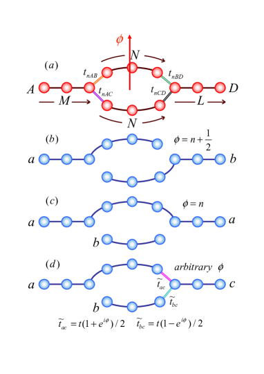
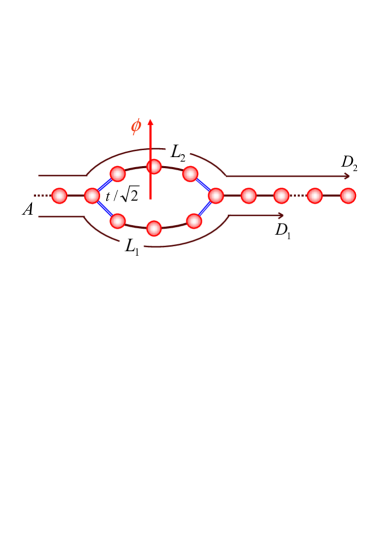
In this subsection, we consider the interferometer model $\{A,B,C,D\}$ for Bloch electron, illustrated schematically in Fig. 8(a). This quantum interferometer consists of two chains $A,D$ and one ring $\{B,C\}$ with one end of each chain connecting to two opposite point of the ring. The ring is threaded by a magnetic flux $\phi$ in the unit of flux quanta. The Hamiltonian reads

$$H=H_{A}+H_{D}+H_{B}+H_{C}+H_{joint}$$ (58)

where $N_{A}=M$, $N_{D}=L$, $N_{B}=$ $N_{C}=N$, $t_{j}^{[A]}=$ $t_{j}^{[D]}=t$, $t_{j}^{[B]}=$ $t\exp(i\Phi_{B,j+1})$, and $t_{j}^{[C]}=$ $t\exp(-i\Phi_{C,j+1})$. The connection Hamiltonian reads

$$H_{joint} = -(t_{nAB}a_{A,M}^{{\dagger}}a_{B,1}e^{i\Phi_{B,1}}+t_{nAC}a_{A,M}^{{\dagger}}a_{C,1}e^{-i\Phi_{C,1}}$$ (59)

$$+t_{nBD}a_{B,N}^{{\dagger}}a_{D,1}e^{i\Phi_{B,N+1}}+$$

$$t_{nCD}a_{C,N}^{{\dagger}}a_{D,1}e^{-i\Phi_{C,N+1}}+H.c.).$$

Here, $\Phi=$ $\sum_{l=1}^{N+1}\Phi_{B,l}$ $+\sum_{l=1}^{N+1}\Phi_{C,l}$ $=2\pi\phi$ is the sum of $\Phi$ along the ring.

In this section, we investigate the basic properties of the flux-controlled interferometer. Similarly, we will find out that there still exist some analytical results, which reveal the dynamics of such network for the appropriate parameters.

V.2 Reduction of the interferometer network

Figure 8: (Color on line) (a) The $\phi$-shaped Bloch electron network with an input chain $A$, an output chain $D$ and a ring ${B,C}$ threaded by a magnetic flux. (b) When $t_{nAB}=t_{nCD}=t\cos\theta$, $t_{nAC}=t_{nBD}=t\sin\theta$ and $\phi=n+1/2$, the $\phi$-shaped Bloch electron network can be decoupled into two virtual homogeneous linear chains $a$ and $b$ with length $M+N$ and $N+L$ respectively. (c) When $t_{nAB}=t_{nBD}=t\cos\theta$, $t_{nAC}=t_{nCD}=t\sin\theta$ and $\phi=n$, the $\phi$-shaped Bloch electron network can be decoupled into a long virtual homogeneous linear chain $a$ with length $M+N+L$ and a short virtual homogeneous linear chain $b$ with length $N$. (d) If $t_{nAB}=t_{nAC}=t_{nBD}=t_{nCD}=t/\sqrt{2}$, for an arbitrary $\phi$, the network can be decoupled into three virtual homogeneous linear chains $a$, $b$ and $c$. They connect with each other by the hopping integrals $\widetilde{t}_{ac}$ and $\widetilde{t}_{bc}$.

To reduce the network of interferometers, the four sets of new fermion operator

$$\widetilde{a}_{a,j}^{{\dagger}} = a_{A,j}^{{\dagger}},$$

$$\widetilde{a}_{a,M+l}^{{\dagger}} = \cos\theta e^{-i\varphi_{B}^{l}}a_{B,l}^{{\dagger}}+\sin\theta e^{i\varphi_{C}^{l}}a_{C,l}^{{\dagger}},$$

$$\widetilde{a}_{b,l}^{{\dagger}} = \sin\theta e^{-i\varphi_{B}^{l}}a_{B,l}^{{\dagger}}-\cos\theta e^{i\varphi_{C}^{l}}a_{C,l}^{{\dagger}},$$

$$\widetilde{a}_{c,s}^{{\dagger}} = e^{i\varphi_{C}^{N+1}}a_{D,s}^{{\dagger}},$$ (60)

for $j\in[1,M]$, $l\in[1,N]$, and $s\in[1,L],$ are introduced to satisfy

$$\left\{\widetilde{a}_{a,M+j},\widetilde{a}_{b,j}^{{\dagger}}\right\}=0.$$ (61)

Here,

$$\varphi_{\alpha}^{j}=\sum_{l=1}^{j}\Phi_{\alpha,l},(\alpha=B,C),$$ (62)

is the sum of the phase.

The inverse transformation of the above Eqs. (60) reduces the Hamiltonian (58) into

$$H = \widetilde{H}_{a}+\widetilde{H}_{b}+\widetilde{H}_{d}$$

$$-t\sum_{j=1}^{N-1}(\widetilde{a}_{a,M+j}^{{\dagger}}\widetilde{a}_{a,M+j+1}+H.c.)$$

$$-[(t_{nAB}\cos\theta+t_{nAC}\sin\theta)\widetilde{a}_{a,M}^{{\dagger}}\widetilde{a}_{a,M+1}$$

$$+(-t_{nAB}\sin\theta+t_{nAC}\cos\theta)\widetilde{a}_{a,M}^{{\dagger}}\widetilde{a}_{b,1}$$

$$+(t_{nBD}\cos\theta e^{i\Phi}+t_{nCD}\sin\theta)\widetilde{a}_{a,M+N}^{{\dagger}}\widetilde{a}_{c,1}$$

$$+(-t_{nBD}\sin\theta e^{i\Phi}+t_{nCD}\cos\theta)\widetilde{a}_{b,N}^{{\dagger}}\widetilde{a}_{c,1}+H.c.]$$

where $N_{a}=M$, $N_{b}=N$, and $N_{c}=L$. Now we concentrate on two special cases with different $\phi$ and other parameters:

V.2.1 Case: $\phi=n+\frac{1}{2}$, $t_{nAB}=t_{nCD}=t\cos\theta$, $t_{nAC}=t_{nBD}=t\sin\theta$

It is obvious that $\exp(i\Phi)=-1$. The Hamiltonian can be rewritten as

$$H = -t(\sum_{j=1}^{M+N-1}\widetilde{a}_{a,j}^{{\dagger}}\widetilde{a}_{a,j+1}+\sum_{j=1}^{L-1}\widetilde{a}_{c,j}^{{\dagger}}\widetilde{a}_{c,j+1}$$

$$+\sum_{j=1}^{N-1}\widetilde{a}_{b,j}^{{\dagger}}\widetilde{a}_{b,j+1}+\widetilde{a}_{b,N}^{{\dagger}}\widetilde{a}_{c,1}+H.c.).$$

We define the new fermion operator

$$\widetilde{a}_{b,N+j}^{{\dagger}}=\widetilde{a}_{c,j}^{{\dagger}},(j\in[1,L])$$ (65)

to extend the virtual chain $b$. Its Hamiltonian

$$H=\widetilde{H}_{a}+\widetilde{H}_{b}$$ (66)

is given by the parameters $N_{a}=M+N$ and $N_{b}=N+L$.

From the reduced Hamiltonian (66), we can see that the interferometer network is decoupled into two imaginary linear chains with homogeneous couplings $t$. The set of $\{\widetilde{a}_{a,j}^{{\dagger}}\mid j\in[1,N+M]\}$ defines one of them with length $M+N$ sites, and the set $\{\widetilde{a}_{a,j}^{{\dagger}}\mid j\in[1,N+L]\}$ defines the other one with length $N+L$. As illustrated schematically in Fig. 8(b).

V.2.2 Case: $\phi=n$, $t_{nAB}=t_{nBD}=t\cos\theta$, $t_{nAC}=t_{nCD}=t\sin\theta$

In this case, the Hamiltonian becomes

$$H = -t(\sum_{j=1}^{M+N-1}\widetilde{a}_{a,j}^{{\dagger}}\widetilde{a}_{a,j+1}+\sum_{j=1}^{L-1}\widetilde{a}_{c,j}^{{\dagger}}\widetilde{a}_{c,j+1}$$

$$+\sum_{j=1}^{N-1}\widetilde{a}_{b,j}^{{\dagger}}\widetilde{a}_{b,j+1}+\widetilde{a}_{a,M+N}^{{\dagger}}\widetilde{a}_{c,1}+H.c.)$$

with the newly defined operators

$$\widetilde{a}_{a,M+N+j}^{{\dagger}}=\widetilde{a}_{c,j}^{{\dagger}},(j\in[1,L])$$ (68)

the reduced Hamiltonian

$$H=\widetilde{H}_{a}+\widetilde{H}_{b}$$ (69)

describe an extended virtual chain of length $N_{a}=M+N+L$ and another of $N_{b}=N$.

It is clear that, when the conditions

$$t_{nAB} = t_{nBD}=t\cos\theta$$

$$t_{nAC} = t_{nCD}=t\sin\theta$$

$$\phi = n$$ (70)

are satisfied, the interferometer network is decoupled into two imaginary linear chains with length $M+N+L$ sites and $N$ sites respectively. See also Fig. 8(c).

V.2.3 Case: arbitrary $\phi$, $t_{nAB}=t_{nAC}=$ $t_{nBD}=t_{nCD}$ $=\frac{t}{\sqrt{2}}$

Under this condition, the Hamiltonian is reduced as

$$H=\widetilde{H}_{a}+\widetilde{H}_{b}+\widetilde{H}_{c}+\widetilde{H}_{joint}$$ (71)

where $N_{a}=M+N$, $N_{b}=N$, and $N_{c}=L$.

Here, the joint Hamiltonian is

$$\widetilde{H}_{joint} = -t[e^{i\frac{\Phi}{2}}\cos\left(\frac{\Phi}{2}\right)\widetilde{a}_{a,M+N}^{{\dagger}}\widetilde{a}_{c,1}$$ (72)

$$-ie^{i\frac{\Phi}{2}}\sin\left(\frac{\Phi}{2}\right)\widetilde{a}_{b,N}^{{\dagger}}\widetilde{a}_{c,1}+H.c.].$$

while the sub-Hamiltonians $\widetilde{H}_{a}$, $\widetilde{H}_{b}$ and $\widetilde{H}_{c}$ present three homogeneous virtual linear chains $\{a,b,c\}$ with length $M+N$, $N$ and $L$ respectively. In $\widetilde{H}_{joint}$, there exists a connection interaction $\exp(i\Phi/2)\cos\left(\Phi/2\right)$ between the two end sites of virtual chain $a$ and $c$. Meanwhile, there exists another connection interaction $-i\exp(i\Phi/2)\sin(\Phi/2)$ between the two end sites of virtual chain $b$ and $c$. The geometry of such network is illustrated in Fig. 8(d). Obviously in the virtual space, such network is equivalent to the $Y$-shaped beam splitter with different lengths of output arms and complex joint hopping constants controlled by the flux $\Phi$. From the discussion about $Y$-shaped network, we have known that the lengths of output arms do not affect the feature as beam splitter for local input wave packet. In the following we will investigate property of such $Y$-shaped network by considering equi-length case for simplicity.

V.3 Y-shaped Beam splitter controlled by $\Phi$

Now we consider a $Y$-shaped network $\{A,B,C\}$ with complex joint hopping constants. The model Hamiltonian reads

$$H=H_{A}+H_{B}+H_{C}+H_{joint}$$ (73)

where $N_{A}=L$, $N_{B}=N_{C}=N$, and $t_{j}^{[A]}=$ $t_{j}^{[B]}=$ $t_{j}^{[C]}=t$. The joint Hamiltonian

$$H_{joint}=-(t_{AB}a_{A,L}^{{\dagger}}a_{B,1}+t_{AC}a_{A,L}^{{\dagger}}a_{C,1}+H.c.),$$

describes the connections with the complex hopping integrals

$$t_{AB}=te^{-i\frac{\Phi}{2}}\cos\left(\frac{\Phi}{2}\right),t_{AC}=ite^{-i\frac{\Phi}{2}}\sin\left(\frac{\Phi}{2}\right).$$ (74)

Interestingly, if we get rid of the exponential terms in the hopping integrals, i.e., $t\cos\left(\Phi/2\right)$, $t\sin\left(\Phi/2\right)$, we recover the matching condition (26) in the original $Y$-shaped beam splitter $t_{AB}^{2}+t_{AC}^{2}=t^{2}$. In order to decouple this network, we introduce three communitative sets of fermion operators

$$\widetilde{a}_{a,l}^{{\dagger}} = a_{A,l}^{{\dagger}},$$

$$\widetilde{a}_{a,L+j}^{{\dagger}} = e^{i\frac{\Phi}{2}}[\cos\left(\frac{\Phi}{2}\right)a_{B,j}^{{\dagger}}-i\sin\left(\frac{\Phi}{2}\right)a_{C,j}^{{\dagger}}],$$

$$\widetilde{a}_{b,j}^{{\dagger}} = e^{-i\frac{\Phi}{2}}[i\sin\left(\frac{\Phi}{2}\right)a_{B,j}^{{\dagger}}+\cos\left(\frac{\Phi}{2}\right)a_{C,j}^{{\dagger}}],$$

for $l\in[1,L]$ and $j\in[1,N]$.

The inverse transformations of Eqs. (LABEL:tran3) result in the reduction of Hamiltonian in terms of $\widetilde{a}_{a,j}^{{\dagger}}$, $\widetilde{a}_{a,L+j}^{{\dagger}}$, and $\widetilde{a}_{b,j}^{{\dagger}}$:

$$H=\widetilde{H}_{a}+\widetilde{H}_{b}$$ (76)

where $N_{a}=L+N$ and $N_{b}=N$.

Thus this kind of $Y$-shaped Bloch electron network is also decoupled into two imaginary chains. Similarly, we apply the beam splitter to the special Bloch electron GWP $\left|\psi_{A}(N_{0})\right\rangle$. At a certain time $\tau$, such GWP evolves into

$$\left|\Psi(\tau)\right\rangle \sim \cos\left(\frac{\Phi}{2}\right)\left|\psi_{B}(N_{\tau})\right\rangle$$ (77)

$$-i\sin\left(\frac{\Phi}{2}\right)\left|\psi_{C}(N_{\tau})\right\rangle,$$

where $N_{\tau}=N_{0}+2t\tau-L$. This means that the beam splitter can split the GWP into two cloned GWPs completely with the probabilities

$$\left|\left\langle j_{B}\right.\left|\psi_{B}(N_{\tau})\right\rangle\right|^{2} = \cos^{2}\frac{\Phi}{2};$$

$$\left|\left\langle j_{C}\right.\left|\psi_{C}(N_{\tau})\right\rangle\right|^{2} = \sin^{2}\frac{\Phi}{2},$$ (78)

which can be controlled by the external flux $\phi$.

V.4 AB effect in a solid system

This virtual model of interferometer network is very similar to the second type of $Y$-shaped beam splitter we discussed before. The only difference between them is that in this virtual model the lengths of the two legs are unequal. Fortunately, by appropriately choosing $\alpha$, the width of the wave packet, the GWP can be regarded as a classical electron. It not only propagates along a homogeneous chain without spreading approximately, but also does not regard the length of the chain. Now we prepare such a moving GWP at the input leg. When it reaches to the node, it will be split into two cloned GWPs with the amplitudes of $\cos^{2}(\Phi/2)$ and $\sin^{2}(\Phi/2)$ respectively. According to our discussion above, the sub-GWP with the amplitude of $\sin^{2}(\Phi/2)$ will be reflected by the opposite node of the ring, but the other sub-GWP with the amplitude of $\cos^{2}(\Phi/2)$ will move onto the output leg directly. So some time later we will receive a cloned GWP with the probability $\cos^{2}(\Phi/2)$ at the output leg.

The interferometer based on Bloch electron network can be regarded as a mimic of AB effect ABeffect experimental device in a solid system illustrated in Fig. 9(a). Here, the initial GWP

$$\left|\psi_{A}(N_{0})\right\rangle=\frac{1}{\sqrt{\Omega_{1}}}\sum_{j=1}^{M}e^{-\frac{\alpha^{2}}{2}(j-N_{0})^{2}}e^{i\frac{\pi}{2}j}\left|j\right\rangle$$ (79)

is taken as a good example to demonstrate the physical mechanism of such setup.

We first focus on the GWP at the input site $N_{0}=A$ and detected it later on a distant site $D_{1}$ or $D_{2}$. The maximal probability of the GWP in some certain site $j$ is

$$|\psi(j,\alpha)|_{\max}^{2}=\max\{\left|\left\langle j\right|e^{-iH\tau}\left|\psi_{A}(N_{0})\right\rangle\right|^{2}\}$$ (80)

Thus we can define the relative probability $Q$ as a function of $\alpha$, the magnetic flux $\phi$, and the site of the detector $j$,

$$Q(j,\phi,\alpha)=\frac{|\psi(j,\alpha)|_{\max}^{2}}{|\psi(A,\alpha)|_{\max}^{2}}.$$ (81)

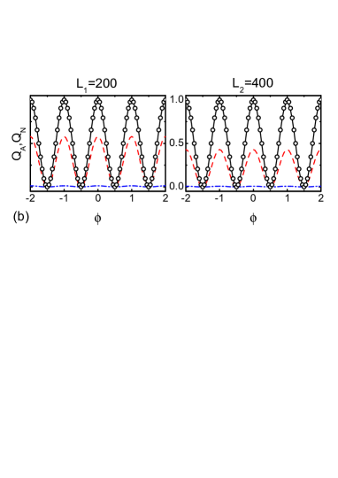
Obviously, $Q$ is an observable physical quantity, which describes the AB effect and the influence of lattice scattering. Numerical simulation of $Q(D_{1},\phi,\alpha)$ and $Q(D_{2},\phi,\alpha)$ for different initial GWP with half-width $\Delta=16.65$, $(\alpha=0.1)$, $\Delta=5.55$, $(\alpha=0.3)$, and $\Delta=1$, $(\alpha=\infty)$ are plotted in Fig. 9(b). Here, the optical paths between the input site and the detector-sites are $L_{1}=200$, $L_{2}=400$. The ring of the system is threaded by a magnetic flux $\phi\in[-2,2]$. The numerical results show that the relative probabilities $Q$ are periodic in the magnetic flux $\phi$ with a period of unit flux quantum $\Phi_{0}=h/e$. This is the so called AB effect in a solid system. At $\phi=$integer, our previous discussion shows that the interferometer network of Bloch electron model is decoupled into one long chain and one short chain. The initial GWP localized in the input arm can be transmitted to the detector-arm without any reflection. Consequently, the relative probability $Q$ reaches its maximum of the curve. On the other hand, when $\phi$ is a half-integer, the initial GWP cannot be transmitted to the detector-arm. Thus, the corresponding $Q$ equals to its minimum zero.

Then we consider the GWPs with different half-width $\Delta=2\sqrt{\ln 2}/\alpha$. If $\Delta$ is larger, the GWP is localized in the linear dispersion regime more exactly. In this case, it can be well transferred without spreading YS1 ; or in another point of view, it is a free particle which will not be scattered by the lattice. We can see from the numerical results, $Q=$ $(1+\cos\Phi)/2$, the maximum $Q$ of $\Delta=16.65$, $(\alpha=0.1)$ is approximately equals to $1$. Otherwise, a GWP with smaller $\Delta$, i.e., $\Delta=5.55$, $(\alpha=0.3)$ is scattered by the lattice severely, so the relative probability $Q$ of which are smaller than $Q$ of wider GWP. It is reasonable that when the optical path is longer, the influence of lattice scattering is larger, the relative probability $Q$ is smaller. The black dot dash line also shows that in large $\alpha$ limit, $Q$ are approximately equal to zero. Therefore, a GWP localized beyond the linear dispersion regime is not suitable for demonstrating the AB effect experiment in a solid system.

To sum up, when the half-width of the initial wave packet is narrower or the detect-length is longer, the relative probability $Q$ is smaller, the AB effect is weaker to be observed. From these results, we get two possible reasons why we cannot observe AB effect in a macroscopically solid system. Firstly, we do not choose an appropriate wave packet. Secondly, the total site of the macroscopically solid system is so large that the influence of lattice scattering cannot be ignored. To solve these problems and to realize AB effect in a solid system, we should choose a wider GWP mentioned in our previous work YS1 . At the same time, we should decrease the optical paths between the input site and the detector-sites.

Figure 9: (Color on line) (a) The schematic illustration for the mimic A-B effect device in a solid system. (b) The comparison of relative probability $Q$ as a function of the magnetic flux $\phi$. The half-width of the initial wave packets are 16.65 ($\alpha=0.1$, blue solid line), 5.55 ($\alpha=0.3$, red dash line), 1 ($\alpha=\infty$, black dot dash line). The optical paths between the input site $A$ and the detector sites $D_{1}$, $D_{2}$ are $L_{1}=200$ (left), $L_{2}=400$ (right). It shows that the relative probability $Q$ are periodic in the magnetic flux $\phi$ with a period of unit flux quantum $\Phi_{0}=h/e$. When the half-width of the initial wave packet is narrower or the optical path is longer, the relative probability $Q$ is smaller, the A-B effect is weaker.

VI Applications for spin network

In the above discussion, we studied the fermion systems where the Bloch electrons move along the quantum lattice network. We consider various geometrical configurations of TBN that are analogous to quantum optical devices, such as beam splitters and interferometers. In this section, we will apply the results obtained for TBN to another analogue system, spin network (SN) where the spin wave acts as the Bloch electron.

The basic setup of a SN is constructed topologically by the linear spin chains and the various connections between the ends of them. Here, we consider the spin-$1/2$ $XY$ model, in which only the nearest neighbor (NN) coupling term is taken into account. The Hamiltonian of a SN reads

$$H^{s}=\sum\limits_{l}H_{l}^{s}+H_{joint}^{s},$$ (82)

where the Hamiltonians of leg $l$ consisting of $N_{l}$ spins and the joints are

$$H_{l}^{s} = H_{l}^{s}(J_{l},N_{l})\circeq\sum_{j=1}^{N_{l}-1}J_{j}^{[l]}(S_{l,j}^{+}S_{l,j+1}^{-}+H.c.),$$

$$H_{joint}^{s} \equiv J_{ji}^{[lm]}S_{l,j}^{+}S_{m,i}^{-}+H.c..$$ (83)

Here, $S_{l,j}^{\pm}$ are the Pauli spin operators acting on the internal space of electron on the $j$th site of the $l$th leg. Although the SNs and TBNs have the same structure, the physics should be different due to the difference of the intrinsic statistical properties. Then the analytical conclusions for TBN are not available to SN. However, in the context of state transfer, only the dynamics of the single-magnon is concerned. Notice that for Hamiltonian (82), the $z$-component of the total spin $S^{z}=\sum\nolimits_{l,i}S_{l,i}^{z}$ is conserved, i.e. $[S^{z},H^{s}]=0$. Thus in the invariant subspace with $S^{z}=(\sum\nolimits_{l}N_{l}-1)/2$, this model can be mapped into single-particle TBN.

VII Conclusion and remark

In summary, we studied various geometrical configurations of tight-binding networks for the fermion systems. It is found that the lattice networks for moving GWPs are analogous to quantum optical devices, such as beam splitters and interferometers. In practice, our coherent quantum network for electronic wave can be implemented by an array of quantum dots, Josephson junctions or other artificial atoms. It will enable an elementary quantum device for scalable quantum computation, which can coherently transfer quantum information among the integrated qubits. The observable effects for electronic wave interference may be discovered in the dynamics of magnetic domain in some artificial quantum material.

In the above studies, we only consider the spinless Bloch electron. Actually, all the conclusions we obtained can be extended to the networks of spin-$1/2$ electrons, if the external magnetic field does not exert any forces or torques on the magnetic moment of spin, but only a phase on the wave function of electron. The Hamiltonian of such system has the similar form with (1) and (4) under the transformation $a_{j}^{{\dagger}}a_{i}\longrightarrow\sum_{\sigma=\pm 1}a_{j,\sigma}^{{\dagger}}a_{i,\sigma}$. Note that, for the new Hamiltonian, the spin of electron is a conservative quantity that cannot be influenced during the propagation YS1 . The electronic wave packet with spin polarization is an analogue of photon “flying qubit”, where the quantum information was encoded in its two polarization states. Thus, these networks can function as some optical devices, such as beam splitters and interferometers. These are expected to be used as quantum information processors for the fermion system based on the possible engineered solid state systems, such as the array of quantum dots, Josephson junctions or other artificial atoms that can be implemented experimentally.

This work is supported by the NSFC with grant Nos. 90203018, 10474104 and 60433050; and by the National Fundamental Research Program of China with Nos. 2001CB309310 and 2005CB724508.

References

- (1) D. Bouwnmeester, A. Ekert, A. Zeilinger(Eds.), “The Physics of Quantum Information”, Springer, Berlin, 2000.
- (2) M.A. Nielsen , I.L. Chuang, ”Quantum Computation and Quantum Information”. Cambridge University Press, Cambridge, U.K. 2000.
- (3) S. Bose, Phys. Rev. Lett. 91, 207901 (2003); S. Bose, B-Q. Jin and V. E. Korepin, Phys. Rev. A 72, 022345 (2005); S. Bose, Phys. Rev. Lett. 91, 207901 (2003); M-H. Yung and S. Bose, Phys. Rev. A 71, 032310 (2005).
- (4) V. Subrahmanyam, Phys. Rev. A 69, 034304 (2004).
- (5) M. Christandl, N. Datta, A. Ekert and A. J. Landahl, Phys. Rev. Lett. 92, 187902 (2004)
- (6) C. Albanese, M. Christandl, N. Datta and A. Ekert, Phys. Rev. Lett. 93, 230502 (2004)
- (7) T. J. Osborne and N. Linden, Phys. Rev. A 69, 052315 (2004).
- (8) Y. Li, T. Shi, B. Chen, Z. Song, C.P. Sun, Phys. Rev. A 71, 022301 (2005).
- (9) T. Shi, Y. Li, Z. Song, and C.P. Sun, Phys. Rev. A 71, 032309 (2005)
- (10) Z. Song, C.P. Sun, Low Temperature Physics 31, 686 (2005).
- (11) M.B. Plenio, F. L. Semiao, New. J. Phys. 7, 73 (2005)
- (12) J. E. Avron; A. Raveh and B. Zur, Rev. Mod. Phys. 60, 873 (1988); C. H. Wu, G. Mahler, Phys. Rev. B 43, 5012 (1991); J. Vidal, G. Montambaux and B. Doucot, Phys. Rev. B 62, R16294 (2000); P. S. Deo and A. M. Jayannavar, Phys. Rev. B 50, 11629 (1994).
- (13) A. Kay and M. Ericsson, New J. Phys. 7, 143 (2005); G. D. Chiara, R. Fazio, C. Macchiavello, S. Montangero and G. M. Palma, Phys. Rev. A 72, 012328 (2005); M. Paternostro, G. M. Palma, M. S. Kim and G. Falci, Phys. Rev. A 71, 042311 (2005).
- (14) R. A. Webb, S. Washburn, C. P. Umbach, and R. B. Laibowitz, Phys. Rev. Lett. 54, 2696 (1985); V. Chandrasekhar, M. J. Rooks, S. Wind, and D. E. Prober, Phys. Rev. Lett. 55, 1610 (1985).
- (15) M.B. Plenio, J. Hartley and J. Eisert, New J. Phys. 6, 36 (2004); A Perales, M.B. Plenio, J. Opt. B 7, S601-S609 (2005).
- (16) N. Byers and C.N. Yang, Phys. Rev. Lett. 7, 46 (1961); H. T. Nieh, G. Su, B-H. Zhao, Phys. Rev. B 51, 3760 (1995).
- (17) D. Langbein, Phys. Rev. 180, 633 (1969); G-Y. Oh, J. Korean Phys. Soc. 42, 714 (2003).
- (18) R. Peierls, Z. Physik 80, 763 (1933).
- (19) S. Yang, Z. Song, and C.P. Sun, Phys. Rev. A 73, 022317 (2006).
- (20) R. Loudon, The quantum theory of light, (Oxford, 2000); M.O. Scully and M.S. Zubairy, Quantum Optics, (Oxford, 1997).
- (21) J.D. Franson; Phys. Rev. A 56, 1800-1805 (1997); K. Jacobs and P.L. Knight; Phys. Rev. A 54, R3738(1996); T. Wang, M. Kostrun, and S.F. Yelin; Phys. Rev. A 70, 053822 (2004).
- (22) M. Zukowski, A. Zeilinger, and M.A. Horne, Phys. Rev. A 55, 2564(1997); J.L. van Velsen, Phys. Rev. A 72, 012334 (2005).
- (23) H. Rauch, W. Treimer, and U. Bonse, Phys. Lett. A 47, 369 (1974).
- (24) D. Cassettari, B. Hessmo, R. Folman, T. Maier, and J. Schmiedmayer, Phys. Rev. Lett. 85, 5483(2000); U. V. Poulsen and K. Momer, Phys. Rev. A 65, 033613 (2002); D. C. E. Bortolotti and J.L. Bohn; Phys. Rev. A 69, 033607 (2004).
- (25) F. Burgbacher and J. Audretsch; Phys. Rev. A 60, R3385(1999); N.M. Bogoliubov, A. G. Izergin, N.A. Kitanine, A.G. Pronko, and J. Timonen; Phys. Rev. Lett. 86, 4439 (2001)
- (26) X. Wang and P. Zanardi, Phys. Lett. A 301, 1 (2002); X. Wang, Phys. Rev. A 66, 034302 (2002).
- (27) X-F. Qian, Y. Li, Y. Li, Z. Song, and C.P. Sun, Phys. Rev. A 72, 062329 (2005).
- (28) Y. Aharonov and D. Bohm, Phys. Rev. 115, 485 (1959).