Density Matrix Tomography of Entangled Electron and Nuclear Spin States in $\mathrm{{}^{15}N@C_{60}}$

Abstract

We discuss details of the preparation and detection of entangled electron-nuclear spin states in $\mathrm{{}^{15}N@C_{60}}$ together with a quantitative evaluation of the complete density matrix. All four Bell states of a two qubit subsystem were analyzed. In addition we find a quantum critical temperature of $T_{q}=7.73~{}K$ for this system at an electron spin resonance frequency of $95~{}GHz$.

I Introduction

In recent years quantum information theory has come to exciting new ideas in the fields of quantum teleportation bennett:93 ; bouwmeester:97 , quantum cryptography bennett:92 and quantum computation deutsch:85 ; deutsch:92 . It was stimulated enormously by the discovery of the factoring shor:97 ; vandersypen:01 and searching algorithms grover:97 ; chuang:98b , which demonstrate that a quantum computer is capable of tasks, that are impossible to solve on a classical computer. Consequently, over the past few years various physical systems were examined or proposed for their potential use as hardware for quantum computing. These include ions confined to an electromagnetic trap cirac:95 ; monroe:95 , photons knill:01 , doped semiconductors kane:98 , Cooper pair states in superconductors shnirman:97 ; nakamura:99 , Josephson junctions mooij:99 ; friedmann:00 , and nuclear spins in liquids (NMR quantum computing) cory:97 ; cory:98a ; gershenfeld:97a ; knill:98a ; jones:98 ; warren:97 ; mehring:99 .

One of the most interesting components in many quantum algorithms are nonlocal quantum correlations that violate our conception of the classical world. These so called entangled states have been discussed for a long time einstein:35 ; bell:64 ; greenberger:89 ; mermin:90 ; lloyd:98 . Experimental preparations of entangled states of photons have been publishedzeilinger:97 ; tittel:98a . The pseudo entanglement of three coupled nuclear spins in the so-called Greenberger-Horne-Zeilinger (GHZ) greenberger:90 state was demonstrated by NMRlaflamme:98 ; nelson:00 ; teklemariam:01 ; teklemariam:02 . Entanglement was also achieved among ions confined in an electromagnetic trap sackett:00 .

In this contribution we present procedures for creating and detecting entanglement between electronic and nuclear spin states in the solid phase of the endohedral fullerene $\mathrm{{}^{14}N@C_{60}}$ which has already been proposed as a basic unit for a scalable quantum computer harneit:02 ; suter:02 . We will show, however, that $\mathrm{{}^{15}N@C_{60}}$ is not a qubit but rather a multi-qubit system and specific addressing schemes must be applied when considering all quantum levels. From its multiple quantum states we will project to a two qubit subsystem and demonstrate the generation of entanglement within this subsystem. The experimental approach is related to the preliminary work presented in mehring:03 where entanglement has been simulated between an electron spin $1/2$ and a nuclear spin $1/2$ of a radical electron in a single crystal of malonic. Due to the strong hyperfine interaction in the system presented here entanglement can be achieved by a factor of thousand shorter time scale than in liquid state NMR. A brief account of our approach to $\mathrm{{}^{14}N@C_{60}}$ was already published in mehring:04a . Here we present further details on the preparation and tomography.

The experiments reported here are carried out in a mixed spin state of an ensemble of spins. Since the complete density matrix in such a system is separable strictly speaking entanglement like in pure quantum states can not be achieved braunstein:99 ; schack:99 . However, the unitary operations applied to the mixed states density matrices are identical to those applied to pure systems and moreover, the resulting density matrices have the same operator structure as the ones of the pure system except for a different overall factor. Therefore these states are called pseudo pure or pseudo entangled cory:97 ; gershenfeld:97a ; knill:98a . In the end we will show that these restrictions can be overcome for the system under investigation for high enough magnetic fields ($95$ GHz electron spin resonance frequency)and low enough temperature( $T=7.73~{}K$) with current technology. The quantum limit where pseudo entangled states become entangled states is therefore well in reach.

Before we start to present the procedures for the more complicated case of $\mathrm{{}^{15}N@C_{60}}$ we sketch as a reminder how entanglement could be achieved in a system of two coupled quantum bits (qubits) represented for example by an electron spin $S=1/2$ and a nuclear spin I=1/2. Starting from the Zeeman product states

$$|m_{S}\,m_{I}\rangle=|\uparrow\uparrow\rangle,\,|\uparrow\downarrow\rangle,\,|\downarrow\uparrow\rangle,\,|\downarrow\downarrow\rangle\,,$$ (1)

entanglement is achieved by applying first a Hadamard transformation $H$ on one spin followed by a controlled not (CNOT) operation. Suppose we start from the pure state $|\downarrow\uparrow\rangle$ we can create the entangled state $\Psi^{+}$ by

$$|\downarrow\uparrow\rangle\stackrel{{\scriptstyle\mbox{H}}}{{\rightarrow}}\frac{1}{\sqrt{2}}|\downarrow\downarrow\rangle+|\downarrow\uparrow\rangle\stackrel{{\scriptstyle\mbox{CNOT}}}{{\longrightarrow}}\frac{1}{\sqrt{2}}|\uparrow\downarrow\rangle+|\downarrow\uparrow\rangle\,.$$ (2)

Depending on the applied unitary transformations and initial states, all four entangled states (Bell-basis) of a two qubit system can be generated by this procedure:

$$\left|\Phi^{\pm}\right\rangle=\frac{1}{2}\left(\left|\uparrow\uparrow\right\rangle\pm\left|\downarrow\downarrow\right\rangle\right)\,,\quad\left|\Psi^{\pm}\right\rangle=\frac{1}{2}\left(\left|\uparrow\downarrow\right\rangle\pm\left|\downarrow\uparrow\right\rangle\right)\,.$$ (3)

As we will see later in detail those transformations can be realized by selective high frequency pulses applied to allowed transitions of the system. We will use in the following the qubit notation $|m_{S}\,m_{I}\rangle=|00\rangle,\,|01\rangle,\,|10\rangle,\,|11\rangle$ as well as the state labelling $|1\rangle,\,|2\rangle,\,|3\rangle,\,|4\rangle$.

I.1 Endohedral fullerene $\mathbf{\mathrm{{}^{15}N@C_{60}}}$

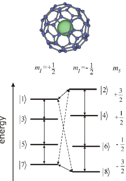
Figure 1: The eight quantum states of a two spin system with $S=3/2$ and $I=1/2$. The arrows denote allowed transitions. The dotted arrows indicate forbidden transitions that belong to the entangled states discussed in this publication. The separation of the energy levels is not to scale.

The experiments were performed on a powder sample of $\mathrm{{}^{15}N@C_{60}}$. The ${}^{15}\mathrm{N}$ atom resides in the center of the $\mathrm{C_{60}}$ molecule. There is no charge transfer from the atom to the cage. The nitrogen atom is paramagnetic due to the half filled $p$ orbital shell with three unpaired electrons which form a total electron spin $S=3/2$. Because of the $\mathrm{{}^{15}N}$ isotope enrichment the nuclear spin of the nitrogen atom is $I=1/2$. The magnetic resonance properties of the sample have already been discussed in detail in almeidamurphy:96 ; weiden:99 . The nitrogen atoms were implanted into the carbon cage by Weidinger and co-workerspietzak:97 by simultaneous evaporation of $\mathrm{C_{60}}$ and ion bombardment onto a cooled target. The sample was purified by high-pressure liquid chromatography.

With the magnetic field oriented along the $z$-axis, the Hamiltonian of this system becomes

$$\mathcal{H}=\hbar\left(\omega_{S}S_{z}+\omega_{I}I_{z}+2\pi a\mathbf{S}\mathbf{I}\right)\,.$$ (4)

where $\omega_{S}$ and $\omega_{I}$ are the Larmor frequencies of electron spin $S=3/2$ and the nuclear spin $I=1/2$. Due to the high symmetry of the molecule the hyperfine interaction $a=-22.08$ MHz is isotropic. This value is larger than for a free nitrogen anderson:59 atom because of the confinement inside the carbon cage. For strong enough magnetic fields, where $|a|,\,\omega_{I}\ll\omega_{S}$, second order contributions to the hyperfine coupling can be neglected and the Hamiltonian is in first order given by:

$$\mathcal{H}=\hbar\left(\omega_{S}S_{z}+\omega_{I}I_{z}+2\pi a\,S_{z}\,I_{z}\right)\,.$$ (5)

The eight eigenvalues of this system are

$$E_{m_{S}\,m_{I}}=\hbar\left(\omega_{S}m_{S}+\omega_{I}m_{I}+2\pi a\,m_{S}\,m_{I}\right)\,,$$ (6)

depending on the spin quantum numbers $m_{S}=\pm 1/2$, $\pm 3/2$ of the electron spin and $m_{I}=\pm 1/2$ of the nuclear spin. The eight eigenstates of the system are given by

$$\left|m_{S}\,m_{I}\right\rangle = \left|1\right\rangle,\left|2\right\rangle,\ldots,\left|8\right\rangle$$

$$= \left|+\frac{3}{2}\,+\frac{1}{2}\right\rangle,\left|+\frac{3}{2}\,-\frac{1}{2}\right\rangle,\ldots,\left|-\frac{3}{2}\,-\frac{1}{2}\right\rangle\,.$$

The corresponding energy level scheme is shown in Fig. 1. Allowed transitions are indicated by arrows. There are in first order three degenerate electron spin transitions ($\Delta m_{S}=\pm 1$) for $m_{I}=+1/2$ and and another three for $m_{I}=-1/2$. Because of this degeneracy the transitions can only be excited simultaneously. There are, however, four nuclear spin transitions ($\Delta m_{I}=\pm 1$). The resulting electron spin resonance (ESR) and electron nuclear double resonance (ENDOR) spectra shown in Fig. 2 verify this level scheme. The lines are labelled according to the spin states $m_{I}$ and $m_{S}$. The ESR spectrum exhibits two lines separated by $22.08$ MHz. The ENDOR spectrum consists of four lines located at $9.67$ MHz, $12.41$ MHz, $31.69$ MHz and $34.54$ MHz.

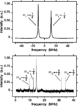
Figure 2: X-band ESR (top) and pulsed-ENDOR spectra mims:65 (bottom) of a powder sample of $\mathrm{{}^{15}N@C_{60}}$ in a magnetic field of $340$ mT. The ESR spectrum was obtained by Fourier transformation of the electron free induction decay (FID).

I.2 Entangled spin states in $\mathrm{{}^{15}N@C_{60}}$

Instead of the four entangled Bell states for two coupled spins 1/2 the endohedral fullerene $\mathrm{{}^{15}N@C_{60}}$ allows for $2\times 12$ entangled states of the type

$$\Psi^{\pm}_{jk}=\frac{1}{\sqrt{2}}\left(\left|j\right\rangle\pm\left|k\right\rangle\right)$$ (8)

with $jk\in\left\{14,23,36,45,58,67,16,25,38,47,18,27\right\}$. Here we will restrict ourselves to the preparation and detection of the following two examples

$$\left|\Psi_{27}^{\pm}\right\rangle = \frac{1}{\sqrt{2}}\left(\left|2\right\rangle\pm\left|7\right\rangle\right)$$

$$= \frac{1}{\sqrt{2}}\left(\left|+\frac{3}{2}\,-\frac{1}{2}\right\rangle\pm\left|-\frac{3}{2}\,+\frac{1}{2}\right\rangle\right)$$

$$\equiv \frac{1}{\sqrt{2}}\left(\left|01\right\rangle\pm\left|10\right\rangle\right)$$

$$\left|\Phi_{18}^{\pm}\right\rangle = \frac{1}{\sqrt{2}}\left(\left|1\right\rangle\pm\left|8\right\rangle\right)$$

$$= \frac{1}{\sqrt{2}}\left(\left|+\frac{3}{2}\,+\frac{1}{2}\right\rangle\pm\left|-\frac{3}{2}\,-\frac{1}{2}\right\rangle\right)$$

$$\equiv \frac{1}{\sqrt{2}}\left(\left|00\right\rangle\pm\left|11\right\rangle\right)$$

Except for the electron spin state with $m_{S}=\pm 3/2$ these states are equivalent to the two qubit Bell states of Eq. (3). The corresponding coherent superpositions are indicated in Fig. 1 by dashed arrows. This defines the fictitious two state subsystem of the electron spin with $|\pm 3/2\rangle$ as one qubit. For the second qubit we consider the $|\pm 1/2\rangle$ states of the nuclear spin. In other words the quantum states $|\pm 3/2\,\pm 1/2\rangle$ represent the four states of our two qubit subsystem. Of course there are other combinations of quantum states that could be regarded as an independent two qubit subsystem. In this sense the quantum system of $\mathrm{{}^{15}N@C_{60}}$ represents a multi qubit system. In the following we will use the qubit notation $|00\rangle$, $|01\rangle$, $|10\rangle$ and $|11\rangle$ for the states $|+\frac{3}{2}\,+\frac{1}{2}\rangle$, $|+\frac{3}{2}\,-\frac{1}{2}\rangle$, $|-\frac{3}{2}\,+\frac{1}{2}\rangle$ and $|-\frac{3}{2}\,-\frac{1}{2}\rangle$.

I.3 $\mathbf{z}$-rotations of the quantum states

In the tomography of quantum states we will apply extensively phase rotations about the $z$-axis. Therefore we investigate here briefly how the different quantum states behave under these phase rotations. A rotation of a spin state of spin $S$ by angle $\varphi_{1}$ and spin $I$ by phase $\varphi_{2}$ around the quantization axis ($z$-axis), corresponds to the unitary transformations

$$U_{S_{z}}=e^{-i\varphi_{1}S_{z}}\quad\mbox{and}\quad U_{I_{z}}=e^{-i\varphi_{2}I_{z}}\,.$$ (11)

Under these transformations the quantum state $|m_{S}\,m_{I}\rangle$ exhibits the following phase variation:

$$U_{S_{z}}\,U_{I_{z}}|m_{S}\,m_{I}\rangle=e^{-i\varphi_{1}S_{z}}e^{-i\varphi_{2}I_{z}}|m_{S}\,m_{I}\rangle\\ =e^{-i\left(m_{S}\varphi_{1}+m_{I}\varphi_{2}\right)}|m_{S}\,m_{I}\rangle$$ (12)

Let us apply these transformations to a superposition state of qubit 1 (subsystem with $m_{S}=\pm 3/2$) which results in

$$\left(|00\rangle+|10\rangle\right)\left(\langle 00|+\langle 10|\right)\stackrel{{\scriptstyle z-\mbox{rot.}}}{{\longrightarrow}}|00\rangle\langle 00|+|10\rangle\langle 10|\\ +e^{-i3\varphi_{1}}|00\rangle\langle 10|+e^{i3\varphi_{1}}|10\rangle\langle 00|.$$ (13)

Note that in the case of an electron spin $S=1/2$ the factor $3$ in front of $\varphi_{1}$ should be replaced by $1$ mehring:03 . Consequently the superposition state of nuclear spin states with $m_{I}=\pm 1/2$ transforms like

$$\left(|10\rangle+|11\rangle\right)\left(\langle 10|+\langle 11|\right)\stackrel{{\scriptstyle z-\mbox{rot.}}}{{\longrightarrow}}|10\rangle\langle 10|+|11\rangle\langle 11|\\ +e^{-i\varphi_{2}}|10\rangle\langle 11|+e^{i\varphi_{2}}|11\rangle\langle 10|.$$ (14)

Note, however, that applying phase rotations to entangled states leads to a different behavior as is demonstrated here for the $\Psi_{27}^{+}$ and $\Phi_{18}^{+}$ states:

$$\left(|01\rangle+|10\rangle\right)\left(\langle 01|+\langle 10|\right)\stackrel{{\scriptstyle z-\mbox{rot.}}}{{\longrightarrow}}|01\rangle\langle 01|+|10\rangle\langle 10|\\ +e^{-i(3\varphi_{1}-\varphi_{2})}|01\rangle\langle 10|+e^{i(3\varphi_{1}-\varphi_{2})}|10\rangle\langle 01|$$ (15a)

$$\left(|00\rangle+|11\rangle\right)\left(\langle 00|+\langle 11|\right)\stackrel{{\scriptstyle z-\mbox{rot.}}}{{\longrightarrow}}|00\rangle\langle 00|+|11\rangle\langle 11|\\ +e^{-i(3\varphi_{1}+\varphi_{2})}|00\rangle\langle 11|+e^{i(3\varphi_{1}+\varphi 2)}|11\rangle\langle 00|.$$ (15b)

The entanglement is evidenced by the combined phase dependence where both phase angles appear as a sum or difference depending on the type of entangled state. In contrast the superposition states of individual spins show only their corresponding single phase behavior. This will be utilized to distinguish different quantum states in the following.

II Experimental

The experiments were performed on a diluted powder sample of $\mathrm{{}^{15}N@C_{60}}$ with a home-built X-band pulsed spectrometer including a slotted tube resonator at about 9.5 GHz. A radio frequency (rf) coil for the excitation of the ENDOR transitions was inserted in the homogeneous region of the microwave field with frequencies ranging from $0-40$ MHz. Both, the microwave channel at X-band frequencies as well as the rf-channel were equipped with arbitrary waveform generators (AWG) which allowed for arbitrary pulse and phase modulation. The quantum states were controlled by applying special unitary transformations implemented as transition selective microwave and radio frequency pulses with rotation angle $\beta$. These pulses are labelled $P_{x;y}^{(\pm)}(\beta)$ for the two electron spin transitions corresponding to $m_{I}=\pm 1/2$ and $P_{x;y}^{(jk)}(\beta)$ for radio frequency pulses on nuclear spin transition between levels $j$ and $k$ (see Fig. 1). The subscripts $x$ or $y$ indicate the phases of the pulses in the corresponding rotating frame. The selective pulses can be written in terms of fictitious spin $1/2$ operators $F_{x;y}^{(\pm)}$ or $F_{x;y}^{(jk)}$, which belong to the transition $(\pm)$ or $(jk)$ vega:77 ; vega:78 as

$$P_{x;y}^{\pm}(\beta)=\exp(-i\beta\,F_{x;y}^{\pm})\quad P_{x;y}^{jk}(\beta)=\exp(-i\beta\,F_{x;y}^{jk})\,.$$ (16)

Pulses with arbitrary phase are expressed as

$$P_{x,\phi_{1}}^{\pm}(\beta) = e^{-i\phi_{1}F_{z}^{\pm}}e^{-i\beta\,F_{x}^{\pm}}e^{i\phi_{1}F_{z}^{\pm}}\quad$$ (17)

$$P_{x,\phi_{2}}^{jk}(\beta) = e^{-i\phi_{2}F_{z}^{jk}}e^{-i\beta\,F_{x}^{jk}}e^{i\phi_{2}F_{z}^{jk}}\,.$$ (18)

All experiments in this contribution were performed at a temperature of $T=50$ K.

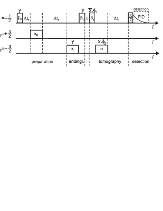
Figure 3: Pulse sequence for preparation and detection of the pseudo entangled state $\Psi^{-}$ in $\mathrm{{}^{15}N@C_{60}}$. The left part refers to the preparation of the pseudo pure state. The middle part represents the preparation and detection of the entangled state. The FID after the selective ESR pulse (right hand side) serves as a monitor signal. The angles $\varphi_{1}$ and $\varphi_{2}$ of the tomography sequence are varied in increments (see text) and are used for separating signals of entangled states from those of individual spins. The waiting times between the pulses were chosen $\Delta t_{1}=5\,\mu$s, $\Delta t_{2}=100\,\mu$s, $\Delta t_{3}=150\,\mu$s and $\tau=40$ ns (see text).

These pulses serve different purposes as is sketched in the general pulse sequence displayed in Fig. 3. The total sequence is separated into four segments, namely (1) preparation of pseudo pure states, (2) creation of entanglement, (3) state tomography and (4) detection via the electron spin free induction decay (FID).

III Pseudo pure states.

III.1 Preparation of pseudo pure states

Like in liquid state NMR quantum computing cory:97 ; gershenfeld:97a ; knill:98a we are dealing here with mixed quantum states and moreover we start initially from a thermal equilibrium state, namely the Boltzmann state which can be expressed as

$$\rho_{\mathrm{B}}=\frac{\mathrm{e}^{-\beta_{\mathrm{B}}\omega_{S}S_{z}}}{\mathrm{Tr}\left\{\mathrm{e}^{-\beta_{\mathrm{B}}\omega_{S}S_{z}}\right\}}$$ (19)

with $\beta_{\mathrm{B}}=\hbar/k_{\mathrm{B}}T$ and where we have applied the approximation $\omega_{S}\gg\omega_{I},a$. With all experiments performed at $T=50$ K and $\hbar\omega_{S}/(k_{\mathrm{B}}T)\approx 0.01\ll 1$ the expression can be further simplified by applying the high temperature approximation which results for our $S=3/2$ and $I=1/2$ system in

$$\rho_{\mathrm{B}}\approx\frac{1}{8}\left(I_{8}-K_{B}S_{z}\right)\quad\mbox{with}\quad K_{B}=\frac{\hbar\omega_{S}}{k_{\mathrm{B}}T}\,.$$ (20)

and where $I_{8}$ represents the $8\times 8$ identity matrix. Eq.(20) can be rewritten as

$$\rho_{\mathrm{B}} \approx \frac{1}{8}\left(1-\frac{1}{2}K_{B}\right)I_{8}+\frac{1}{4}K_{B}\rho_{\mathrm{P}}\quad\mbox{with}\quad$$ (21)

$$\rho_{\mathrm{P}} = \frac{1}{4}I_{8}-\frac{1}{2}S_{z}.$$ (22)

This defines the $8\times 8$ so-called pseudo Boltzmann matrix $\rho_{\mathrm{P}}$ which will be the starting point for preparing pseudo pure initial density matrices.

We treat in the following the preparation of the pseudo pure density matrix $\rho_{\mathrm{P}10}$, from which we will extract finally the two qubit density matrix $\rho_{10}$ with diagonal components $\{0,0,1,0\}$, as an example. It is important to prepare a pseudo pure state which not only resembles the corresponding pure quantum state with the same operator structure but also corresponds to a large nuclear spin alignment which is a prerequisite for reaching a high degree of entanglement. According to Fig. 3 we first apply a pulse $P_{y}^{(-)}(\beta_{0})$ with $\beta_{0}=\arccos(-1/3)=109,47^{\circ}$ at the electron spin transitions for $m_{I}=-1/2$. After a waiting time of $\tau_{1}=5\,\mu$s all transverse components have decayed and a pulse $P_{y}^{(12)}(\alpha_{0})$ pulse with $\alpha_{0}=\pi/2$ at the $1\leftrightarrow 2$ ENDOR transition follows in order to equalize the populations of level 1 and 2. After an additional waiting time of $\tau_{2}=100\,\mu$s all transient components of the density matrix have decayed and the pseudo pure state $\rho_{\mathrm{P}10}$ has been reached with

$$\rho_{\mathrm{P}10}=\left\{\mathbf{0},\mathbf{0},~{}0,\frac{1}{3},~{}\frac{1}{2},\frac{1}{6},\mathbf{1},\mathbf{0}\right\}$$ (23)

where here and in the following we express diagonal density matrices by the diagonal element vector where the elements in bold type correspond to the matrix $\rho_{10}$ of the subsystem $m_{S}=\pm 3/2$ and $m_{I}=\pm 1/2$.

The pseudopure state $\rho_{11}$ can be prepared in a similar way by exciting the electron spin transition with $m_{I}=+1/2$.

Figure 4: Rabi oscillations at the electron spin transitions with $m_{I}=-1/2$. Top: Boltzmann state $\rho_{\mathrm{P}}$. Bottom: After application of a $P_{y}^{(-)}(\beta_{0})$ pulse.

III.2 Tomography of pseudo pure states

The reconstruction of the density matrix of a quantum state by density matrix tomography has already been applied in liquid state NMR quantum computing chuang:98b ; knill:98a ; laflamme:98 ; boulant:02 ; teklemariam:02 ). Here the situation is different because we are dealing with ESR and ENDOR transitions in a solid at low temperatures. In order to verify the proper preparation of the pseudo pure density matrices we have applied Rabi oscillation measurements on different electron and nuclear transitions. This is shown for the pseudopure state $\rho_{10}$ in Fig. 4 as an example. There the magnitude of the electron spin free induction decay (FID) signal is plotted after applying pulses of variable length at particular ESR or ENDOR transitions. The Rabi oscillations decay due to the microwave- or rf-field inhomogeneity. However, their amplitude and initial phase represent the population difference in magnitude and sign of the particular transition where the pulse is applied. The amplitude of the Rabi oscillations was determined by Fourier transformation and integration over the line in the corresponding spectrum. The experimental values were calibrated with respect to the Boltzmann state $\rho_{\mathrm{P}}$ whose amplitude is defined as $A_{\mathrm{P}}\equiv 1/2$. Similar measurements were obtained for state $\rho_{11}$.

Figure 4 shows Rabi oscillations at the ESR transition with $m_{I}=-1/2$. A comparison is made between the Boltzmann state (top) and an inverted state (bottom) after the application of a $P_{y}^{(-)}(\beta_{0})$ pulse. Note the change in amplitude and sign with respect to the Boltzmann state. The level of inversion was determined to -0.329 which results in an angle $\beta_{0}=\arccos(-0.329)\triangleq 109.2^{\circ}$ to be compared with the ideal value $\beta_{0}=\arccos(-1/3)\triangleq 109.5^{\circ}$.

In addition we performed similar Rabi precession experiments at the ENDOR transitions $1\leftrightarrow 2$ and $7\leftrightarrow 8$ of the pseudo pure state $\rho_{\mathrm{P}10}$. From the amplitude of the Rabi oscillations we have determined the corresponding population differences. The deviation from the theoretically expected values can be expressed in terms of deviations of the angles $\beta_{0}$ and $\alpha_{0}$ from their ideal values. By comparing the expected signal strength

$$A_{\mathrm{P}10}^{(12)}=-\frac{9}{80}\cos\alpha_{0}\left(1-\cos\beta_{0}\right)\,$$ (24)

with and without the $P_{y}^{(12)}(\alpha_{0})$ pulse leads to an effective value of $\alpha_{0}=1.55\equiv 88.8^{\circ}$ which reflects a rather small deviation from the ideal value $\alpha_{0}=\pi/2\equiv 90.0^{\circ}$. Deviations of the angles $\alpha_{0}$ and $\beta_{0}$ from their ideal values are not due to misadjusting but are rather caused by microwave- and rf-field inhomogeneities. This affects the diagonal elements of $\rho^{(exp)}_{P10}$ and leads to the following values

$$\rho^{(exp)}_{\mathrm{P}10}=\left\{\mathbf{-0.01},\mathbf{0.01},0,~{}0.33,~{}\frac{1}{2},~{}0.17,\mathbf{1},\mathbf{0.00}\right\}$$ (25)

where negative values arise from experimental errors. After such a data analysis we obtain for the pseudo pure fictitious two qubit density matrix $\rho_{10}$

$$\rho_{10}=\left(\begin{array}[]{cccc}-0.01&0&0&0\\ 0&0.01&0&0\\ 0&0&1&0\\ 0&0&0&0.00\end{array}\right)\,.$$ (26)

The errors are in the last digit. Note that the numbers 1 and $\frac{1}{2}$ derive from $\rho_{\mathrm{P}}$ of the Boltzmann state (see Eq.(21)) and are not changed by the preparation pulses. Matrix elements of those types are written in the following as bare numbers or fractions. In a similar way as the pseudo pure density matrix $\rho_{11}$ was obtained.

These pseudo pure states serve as initial states for the generation of entangled states. $\rho_{10}$ was used to generate the Bell-states $\Psi_{27}^{\pm}$ and $\rho_{11}$ to generate $\Phi_{18}^{\pm}$.

IV Pseudo entangled states

IV.1 Preparation of pseudo entangled states

Pseudo entangled states were prepared according to the pulse sequence depicted in Fig. 3 (central part). Instead of the usual Hadamard transformation a selective $\pi/2$ pulse on a specific nuclear spin transition was applied which has a related effect as the Hadamard transform. The CNOT-gate was implemented by a selective $\pi$-pulse on an electron spin transition. Either $\Psi^{\pm}$ or $\Phi^{\pm}$ states were generated depending on the pseudo pure initial state and the transitions used. In order to distinguish the different Bell states we have used phase rotations of the pulses in the tomography sequence (see Fig. 3) as presented before mehring:03 .

According to equations (I.2) and (I.2) we need to prepare the following density matrices

$$\rho_{\Psi^{\pm}}^{27}=\frac{1}{2}\left|2\pm 7\right\rangle\left\langle 2\pm 7\right|\quad\mbox{and}\quad\rho_{\Phi^{\pm}}^{18}=\frac{1}{2}\left|1\pm 8\right\rangle\left\langle 1\pm 8\right|\,.$$ (27)

Starting from the pseudo pure state $\rho_{\mathrm{P}10}$ first a $\alpha_{1}=\pi/2$-pulse was applied at the nuclear spin transition $7\leftrightarrow 8$ followed immediately by a $\beta_{1}=\pi$-pulse at electron spin transitions with $m_{I}=-1/2$ (see Fig. 3) leading to the following sequence of unitary transformations

$$\rho_{\mathrm{P}\Psi^{\pm}}^{27}=U_{\mathrm{\pm}}^{27}\rho_{\mathrm{P}10}\left(U_{\mathrm{\pm}}^{27}\right)^{\dagger}\quad\mbox{with}\quad U_{\mathrm{\pm}}^{27}=P_{y}^{-}(\mp\pi)\,P_{y}^{78}(+\pi/2)\,.$$ (28)

Under ideal conditions this would result in

$$\rho_{\mathrm{P}\Psi^{\pm}}^{27}=\left(\begin{array}[]{cccccccc}\mathbf{0}&\mathbf{0}&0&0&0&0&\mathbf{0}&\mathbf{0}\\ \mathbf{0}&\mathbf{\frac{1}{2}}&0&0&0&0&\mathbf{\pm\frac{1}{2}}&\mathbf{0}\\ 0&0&0&0&0&0&0&0\\ 0&0&0&\frac{1}{6}&0&0&0&0\\ 0&0&0&0&\frac{1}{2}&0&0&0\\ 0&0&0&0&0&\frac{1}{3}&0&0\\ \mathbf{0}&\mathbf{\pm\frac{1}{2}}&0&0&0&0&\mathbf{\frac{1}{2}}&\mathbf{0}\\ \mathbf{0}&\mathbf{0}&0&0&0&0&\mathbf{0}&\mathbf{0}\\ \end{array}\right)\,$$ (29)

where the elements in bold type again belong to the fictitious two qubit submatrix

$$\rho_{\Psi^{\pm}}=\left(\begin{array}[]{cccc}0&0&0&0\\ 0&\frac{1}{2}&\pm\frac{1}{2}&0\\ 0&\pm\frac{1}{2}&\frac{1}{2}&0\\ 0&0&0&0\\ \end{array}\right)\,.$$ (30)

The two qubit submatrix of the density matrix $\rho_{\mathrm{P}\Psi^{\pm}}^{27}$ is almost identical to $\rho_{\Psi^{\pm}}^{27}$ (see eq. (27)) except for additional diagonal elements outside the fictitious two qubit subsystem.

Similarly we have prepared the $\rho_{\Phi^{\pm}}^{18}$ states by starting from the pseudo pure state $\rho_{\mathrm{P}11}$ and applied a $\pi/2$-pulse on nuclear transition $7\leftrightarrow 8$ followed immediately by a $\pi$-Pulse on electron spin transitions with $m_{I}=+1/2$

$$\rho_{\mathrm{P}\Phi^{\pm}}^{18}=U_{\mathrm{\pm}}^{18}\rho_{\mathrm{P}11}\left(U_{\mathrm{\pm}}^{18}\right)^{\dagger}\quad\mbox{with}\quad U_{\mathrm{\pm}}^{18}=P_{y}^{+}(\pm\pi)\,P_{y}^{78}(+\pi/2)\,$$ (31)

with

$$\rho_{\mathrm{P}\Phi^{\pm}}^{18}=\left(\begin{array}[]{cccccccc}\mathbf{\frac{1}{2}}&\mathbf{0}&0&0&0&0&\mathbf{0}&\mathbf{\pm\frac{1}{2}}\\ \mathbf{0}&\mathbf{0}&0&0&0&0&\mathbf{0}&\mathbf{0}\\ 0&0&\frac{1}{6}&0&0&0&0&0\\ 0&0&0&0&0&0&0&0\\ 0&0&0&0&\frac{1}{3}&0&0&0\\ 0&0&0&0&0&\frac{1}{2}&0&0\\ \mathbf{0}&\mathbf{0}&0&0&0&0&\mathbf{0}&\mathbf{0}\\ \mathbf{\pm\frac{1}{2}}&\mathbf{0}&0&0&0&0&\mathbf{0}&\mathbf{\frac{1}{2}}\\ \end{array}\right)\,$$ (32)

where the elements in bold type again belong to the fictitious two qubit submatrix

$$\rho_{\Phi^{\pm}}=\left(\begin{array}[]{cccc}\frac{1}{2}&0&0&\pm\frac{1}{2}\\ 0&0&0&0\\ 0&0&0&0\\ \pm\frac{1}{2}&0&0&\frac{1}{2}\\ \end{array}\right)\,.$$ (33)

Here we have used a pulse length of $1.6\,\mu$s for the $\pi/2$ radio frequency pulse and 88 ns for the microwave $\pi$-pulse. By this entanglement was prepared within approximately $1.7\,\mu$s starting from the pseudo pure state.

Note that the density matrices $\rho_{\Psi^{\pm}}$ (Eq. (30)) and $\rho_{\Phi^{\pm}}$ (Eq. (33)) correspond to the Bell states defined in Eq. (3). Here we investigated which density matrices are obtained under ideal conditions. In the next section we analyze the experimentally obtained density matrices by performing a density matrix tomography.

IV.2 Density matrix tomography

In the density matrix tomography used here we combine Rabi precession to determine the populations of the quantum levels together with phase incrementation measurements to discriminate between different off-diagonal components.

Since entangled states are not directly observable we need to transform them to an observable state. We therefore apply an entangled state detector consisting for the states $\Psi^{\pm}$ the pulse sequence $P^{(-)}_{x}(-\beta_{1})$ with $\beta_{1}=\pi$ followed by $P^{(78)}_{x}(\alpha)$ with $\alpha=\pi/2$ (see Fig. 3). We note that we always use the same angle $\beta_{1}$ in the preparation and the detection sequence or technically speaking we use the same amplitude and pulsewidth.

IV.2.1 Phase rotation of entangled states

An essential aspect of our type of tomography for distinguishing between the different Bell states is their dependence on $z$-rotations as discussed in section I.3 mehring:03 . Accordingly we have implemented the detection sequence with $P^{-}_{x}(-\pi,~{}\phi_{1})$ and $P^{78}_{x}(\pi/2,~{}\phi_{2})$ pulses. The corresponding unitary transformation of the detection sequence then reads

$$U^{27}_{\mathrm{d}}(\phi_{1},~{}\phi_{2})=P^{78}_{x}(\pi/2,~{}\phi_{2})\,P^{-}_{x}(-\pi,~{}\phi_{1}).$$ (34)

The measured quantity after the detection is the $z$-magnetization of the electron spin subsystem with $m_{I}=-1/2$ in the case of $\Psi_{27}^{\pm}$. The observed signal strength is therefore expected to vary as

$$S_{\Psi}^{\pm}(\phi_{1},\phi_{2}) = -\frac{\mathrm{Tr}\left\{F^{-}_{z}\,U^{27}_{\mathrm{d}}\,\rho_{\mathrm{P}\Psi^{\pm}}^{27}\,U^{27{\dagger}}_{\mathrm{d}}\right\}}{\mathrm{Tr}\left\{\left(F^{-}_{z}\right)^{2}\right\}}$$ (35)

$$= \frac{2}{15}\pm\frac{3}{20}\cos(3\phi_{1}-\phi_{2})$$ (36)

where $F^{-}_{z}$ is the fictitious electron spin 3/2 of the $m_{I}=-1/2$ subsystem. The phase dependence with $(3\phi_{1}-\phi_{2})$ is characteristic for the $\Psi^{\pm}$ states. The variation with $3\phi_{1}$ originates from the $\pm 3/2$ levels.

Similarly we have used the sequence

$$U^{18}_{\mathrm{d}}(\phi_{1},~{}\phi_{2})=P^{78}_{x}(\pi/2,~{}\phi_{2})\,P^{+}_{x}(-\pi,~{}\phi_{1}).$$ (37)

for the detection of the $\Phi_{18}^{\pm}$ states resulting in a detector signal

$$S_{\Phi}^{\pm}(\phi_{1},\phi_{2}) = -\frac{\mathrm{Tr}\left\{F^{+}_{z}\,U^{18}_{\mathrm{d}}\,\rho_{\mathrm{P}\Phi^{\pm}}^{18}\,U^{18{\dagger}}_{\mathrm{d}}\right\}}{\mathrm{Tr}\left\{\left(F^{+}_{z}\right)^{2}\right\}}$$ (38)

$$= \frac{2}{15}\pm\frac{3}{20}\cos(3\phi_{1}+\phi_{2})$$ (39)

for $\Phi_{18}^{\pm}$ and where preparation and detection pulses were applied at the $m_{I}=+1/2$ ESR transitions. The phase variation with $(3\phi_{1}+\phi_{2})$ is characteristic for the $\Phi_{18}^{\pm}$ states.

The phase dependence of the entangled state was measured by repeating the whole pulse sequence shown in Fig. 3 for different values of $\varphi_{1}$ and $\varphi_{2}$. The angles $\varphi_{1}$ and $\varphi_{2}$ were incremented in steps of $\Delta\varphi_{1}$ and $\Delta\varphi_{2}$, leading to phase angles

$$\varphi_{1}(n) = n\,\Delta\varphi_{1}=n\nu_{1}\,\Delta t$$ (40)

$$\varphi_{2}(n) = n\,\Delta\varphi_{2}=n\nu_{2}\,\Delta t$$ (41)

after $n$ steps. We have introduced here a virtual time scale $t=n\,\Delta t$ which defines the virtual frequencies $\nu_{1}$ and $\nu_{2}$. By incrementing both phase angles $\phi_{1}$ and $\phi_{2}$ simultaneously an oscillatory behavior of the detection signal according to eqns. (36) and (39) is expected. In the following we call the corresponding traces, shown in Fig.(5) phase interferograms.

 

Figure 5: Left: Phase interferograms for a complete set of Bell states according to the pulse sequence in Fig.3 with phase incrementation frequencies $\nu_{1}=2.5$ MHz and $\nu_{1}=1.0$ MHz. The experimental traces belong to $\rho_{\mathrm{P}\Psi^{-}}^{27}$ (a) to (c), $\rho_{\mathrm{P}\Psi^{+}}^{27}$(d), $\rho_{\mathrm{P}\Phi^{+}}^{18}$ (e) and $\rho_{\mathrm{P}\Phi^{-}}^{18}$ (f). In the first two interferograms only one of phase angle was incremented: (a): incrementation of $\phi_{2}$, (b): incrementation of $\phi_{1}$. In the interferograms (c) to (f) both phase angles $\phi_{1}$ and $\phi_{2}$ were incremented simultaneously. Right: Corresponding power spectra after Fourier transformation . There is a dominant line at $3\nu_{1}-\nu_{2}$ for the $\rho_{\mathrm{P}\Psi^{\pm}}^{27}$ states and at $3\nu_{1}+\nu_{2}$ for the $\rho_{\mathrm{P}\Phi^{\pm}}^{18}$ states. See text for additional weak lines.

Figure (5) shows phase interferograms and the corresponding Fourier spectra for phase incrementation the two frequencies $\nu_{1}=2.5$ MHz and $\nu_{2}=1.0$ MHz. The presence of entangled states is revealed by dominant lines at $3\nu_{1}-\nu_{2}$ for the $\rho_{\mathrm{P}\Psi^{\pm}}^{27}$ states ((c) and (d)) and at $3\nu_{1}+\nu_{2}$ for the $\rho_{\mathrm{P}\Phi^{\pm}}^{18}$ states ((e) and (f)) in contrast to the single spin phase variations seen in (a) and (b).

The additional weak lines appearing at $\nu_{1}$ and $2\nu_{1}\mp\nu_{1}$ are artifacts due to pulse imperfections. A theoretical analysis shows that the ratio of the amplitudes of the lines at $2\nu_{1}\mp\nu_{1}$ and $3\nu_{1}\mp\nu_{1}$ depends on the deviation $\epsilon_{\beta}$ of the electron spin rotation angle $\beta_{1}$ from $\pi$

$$\frac{A(2\nu_{1}\mp\nu_{2})}{A(3\nu_{1}\mp\nu_{2})}\approx 24\frac{\epsilon_{\beta}^{2}}{\left(16-21\epsilon_{\beta}^{2}\right)}\quad\mbox{with}\quad\epsilon_{\beta}=\beta_{1}-\pi\,.$$ (42)

where terms up to second order in $\epsilon_{\beta}$ were considered. This we have used to quantify the precision of the applied electron spin pulse $\beta_{1}$. For example the mean deviation from the ideal situation for state $\rho_{\mathrm{P}\Psi^{-}}^{27}$ (Fig. 5 (c)) can be determined to be $\left|\overline{\epsilon}_{\beta}\right|=0.23$. This is in accordance with the fact that a perfect $\pi$-pulse does not exist, because microwave field inhomogeneities alone already prevent a complete inversion. $\overline{\epsilon}_{\beta}$ therefore comprises positive as well as negative deviations. Smaller values of $\overline{\epsilon}_{\beta}$ could therefore be achieved by more homogeneous microwave fields. The determination of $\overline{\epsilon}_{\beta}$ as a measure of the precision of the entangled states was performed also for the other Bell states and is an essential part for the estimation of the experimental precision of the created states.

IV.2.2 The diagonal part

The diagonal part of the density matrix of the entangled states was determined by Rabi oscillations in a similar way as already discussed for the pseudo pure states in section III. Here we combine electron spin Rabi oscillations together with nuclear spin Rabi oscillations at the relevant transitions $1\leftrightarrow 2$ and $7\leftrightarrow 8$.

After the preparation of the entangled state a waiting time of $100\,\mu$s was added to let all off-diagonal elements decay. After this a pulse of variable length at the particular transition was added resulting in the observed Rabi oscillations where the initial amplitude is proportional to the difference of the corresponding diagonal matrix elements. The results were calibrated with respect to the previous data obtained for the Boltzmann and pseudo pure state. By applying the appropriate numerical analysis we extracted for the $\rho_{\mathrm{P}\Psi^{-}}^{27}$ state the following values for the effective rotation angles $\alpha_{1}^{-}=86.6^{\circ}$, $\alpha_{1}^{12}=86.8^{\circ}$ and $\alpha_{1}^{78}=88.7^{\circ}$. In this analysis we included the mean deviation $|\overline{\epsilon}_{\beta}|=0.23$ which is legitimate since $\epsilon_{\beta}$ enters the equations only in even powers. Since all three measurements are equally sensitive to experimental errors we have taken their mean value

$$\alpha_{1}=\frac{1}{3}\left(\alpha_{1}^{-}+\alpha_{1}^{12}+\alpha_{1}^{78}\right)=87.4^{\circ}\,.$$ (43)

By combining the previous results for the initial pseudo pure state $\rho_{10}$ from Eq.(LABEL:eqn:diagrho) with the values of $\alpha_{1}$ and $|\epsilon_{\beta}|$ we obtain the complete set of the diagonal elements $r_{j}^{\Psi}$ of the density matrix $\rho_{P\Psi^{-}}^{27}$ as

$$r_{j}^{\Psi}=\left\{\mathbf{-0.01},~{}\mathbf{0.47},~{}0,~{}0.19,~{}\frac{1}{2},~{}0.31,~{}\mathbf{0.52},~{}\mathbf{0.02}\right\}.$$ (44)

The diagonal elements of the corresponding sublevel density matrix $\rho_{\Psi^{-}}$ are printed in bold type. Their experimental error are estimated to be equal or smaller than $\pm 0.05$. The values are therefore in good agreement with the ideal density matrix in Eq. (32). Elements originating from the initial Boltzmann density matrix are unaffected by the pulse sequence are presented by bare numbers or fractions. A similar analysis was made for the diagonal elements of the other Bell states. We remark that this analysis is affected by the decay time of the diagonal terms during the waiting time of $100\,\mu$s introduced between preparation and detection. In order to estimate its influence we measured this decay time to $2.60$ ms which results in a decay by only 4%. We have not corrected for this decay but considered it to be within the experimental error.

IV.2.3 The off-diagonal part

Because we have experimentally determined already both pulse angles of the sequence for preparing the entangled states, namely $\alpha_{1}$ and $\beta_{1}=\pi+\epsilon_{\beta}$, the unitary transformations for the preparation of entanglement are known and could in principle be applied to calculate the corresponding off-diagonal elements of the density matrix. In order to experimentally determine the off-diagonal elements we have, however, applied an alternative tomography sequence to determine the actual values of the off-diagonal elements with respect to the diagonal elements.

In the tomography part of the sequence in Fig. 3 we have incremented the rotation angle $\alpha$ (Rabi oscillation) at the $7\leftrightarrow 8$ transition for different settings of the phase $\phi_{1}$ and a constant value $\phi_{2}$. After Fourier transform of the Rabi oscillations spectra result where their real parts are displayed in Fig. 6 for different values of $\phi_{1}$. Note, however, that the signal now depends on diagonal as well as on off-diagonal elements of the density matrix.

Figure 6: A series of Fourier transformed Rabi oscillations at the $7\leftrightarrow 8$ transition of the $\rho_{\mathrm{P}\Psi^{-}}^{27}$ state for different values of $\phi_{1}$.

Except for an additional $\phi_{2}=90^{\circ}$ phase rotation, in order to be sensitive to ”$\sin\alpha$”-terms, the amplitudes were evaluated in the same way as discussed for the Rabi oscillations.

Figure 7: Amplitudes variation of the Rabi spectra of Fig. 6 versus $\phi_{1}$.

A simple calculation leads to the following expression

$$S_{\Psi^{-}}^{\alpha}=B_{0}+A_{1}\cos{\alpha}-A_{2}\sin{\phi_{1}}+\\ A_{3}\sin\alpha\sin(2\phi_{1}-\phi_{2})-A_{4}\sin\alpha\cos(3\phi_{1}-\phi_{2})\,.$$ (45)

for the detector signal of this type of tomography. Due to the appropriate phase setting combined with selecting the relevant terms of corresponding spectrum after a complex Fourier transform allows us extract only terms with ”$\sin\alpha$” i.e. those two terms with amplitudes $A_{3}$ and $A_{4}$ in Eq. (45) in the data shown in Fig. 7. By using the ratio $A_{3}/A_{4}$ from the phase interferogram in Fig. 5 (c) we were able to determine the amplitude $A_{4}$ from a fit to the data shown in Fig. 7.

The most important matrix element of the entangled state $\rho_{\mathrm{P}\Psi^{-}}^{27}$, namely the matrix element $r_{27}=r_{72}$ enters the $A_{4}$ parameter in the following way

$$A_{4}=-\frac{3}{10}r_{27}\left(\cos\left(\frac{\epsilon_{\beta}}{2}\right)\right)^{3}\,\,\mbox{with}\,\,\epsilon_{\beta}=\overline{\epsilon}_{\beta}=\pm 0.23.$$ (46)

From the knowledge off all other parameters we obtain the value.

$$r_{27}=r_{72}=-0.31\pm{0.04}\,.$$ (47)

This is only $0.64\%$ of the theoretically expected value since from the experimentally known values of the angles $\beta_{1}$ and $\alpha_{1}$ of the preparation sequence and the pseudo pure density matrix one would expect $r_{27}^{\mathrm{th}}=r_{72}^{\mathrm{th}}=-0.49$. The reason for the reduced value is the decoherence of the entangled state during and after preparation and the delay (including finite pulse width) up to the tomography.

IV.2.4 Decoherence

Decoherence reduces the off-diagonal values of the density matrix since the pulse sequence for the preparation and tomography requires finite pulse lengths and a minimum delay $\tau$ between the excitation and the tomography sequence.

Figure 8: Decay of the off-diagonal element $r_{27}$ for state $\rho_{P\Psi^{-}}^{27}$ modulated by double resonance TPPI (time proportional phase incrementation) with frequencies $\nu_{1}=8.0$ MHz, $\nu_{2}=4.0$ MHz. The decay is modulated by the characteristic frequency $3\nu_{1}-\nu_{2}$.

We have measured this decay for the $\Psi^{-}$ state by incrementing the delay time between the preparation sequence and the tomography sequence. The decoherence decay shown in Fig. 8 is modulated by the characteristic frequency $3\nu_{1}-\nu_{2}$ for the $\rho_{\mathrm{P}\Psi^{-}}^{27}$ state imposed by the time proportional phase incrementation (TPPI) procedure drobny:79 ; bodenhausen:80 . Our type of double resonance TPPI was implemented by combined phase increments of $\phi_{1}$ and $\phi_{2}$ in the tomography sequence. In order to purify the decay function from artifacts corresponding to the weak lines in Fig. 5 (c) we have added measurements with $y$ and $-y$ preparation pulses (phase cycling). As a consequence the decay function is solely modulated by the frequency $3\nu_{1}-\nu_{2}$ characteristic for the entangled state $\Psi^{-}$. Other coherent excitations would appear with other phase incrementation frequencies.

By analyzing the decay function in Fig. 8 we were able to determine the time constant of the decoherence of the entangled state to

$$T_{\Psi}=(208\pm 10)\,\mbox{ns.}$$ (48)

Since the process of decoherence is not the subject of this contribution we only remark that it is dominated by an inhomogeneous distribution of the ESR transitions. In order to reconstruct the values of $r_{27}=r_{72}$ right after their preparation we need to evaluate the effective delay time of the tomography sequence. It is comprised of finite pulse width as well as actual delay $\tau$ due to technical constraints. Since the ESR pulses had to be soft in order to avoid cross talk with the other ESR line the corresponding pulse width was $88$ ns which is not short with respect to $T_{\Psi}$. By considering both, the finite pulse width and the delay time $\tau$ we could reconstruct the initial values of $r_{27}=r_{72}$ to

$$\left.r_{27}^{\Psi_{-}}\right|_{\mathrm{initial}}=\left.r_{72}^{\Psi_{-}}\right|_{\mathrm{initial}}=-0.42$$ (49)

This gives a reasonably high degree of entanglement right after creation.

IV.2.5 The complete density matrix

The summary of the density matrix tomography presented here results in the complete density matrix for all four Bell states. Fig. 9 shows a graphical representation of the complete density matrix of $\rho_{\mathrm{P}\Psi^{+}}^{27}$ together with complete initial density matrix $\rho_{P10}$.

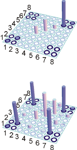
Figure 9: Top: Pseudo pure initial density matrix $\rho_{P10}$. Bottom: Density matrix $\rho_{\mathrm{P}\Psi^{+}}^{27}$

The elements of the two qubit submatrix are enhanced by a darker representation, whereas the other matrix elements are presented lighter. Note that the initial matrix $\rho_{P10}$ already contains diagonal elements in the middle area which are not relevant for the subsystem we are interested in. They are only slightly affected by the entanglement sequence. The errors of the diagonal elements of $\rho_{\mathrm{P}\Psi^{+}}^{27}$ were estimated to be smaller or equal to $\pm 0.05$. The errors of the nominally zero off-diagonal elements are typically smaller than $\pm 0.06$. The nominally zero off-diagonal elements in the two qubit submatrix have errors on the order of $\pm 0.01$. Some of the density matrix elements are unaffected by the preparation sequence are identically zero.

Similar results were obtained for $\rho_{\mathrm{P}\Psi^{+}}^{27}$ and with $\rho_{P11}$ as initial density matrix for the $\rho_{\mathrm{P}\Phi^{\pm}}^{19}$ Bell states. This leads us finally to the following two qubit submatrices corresponding to the two qubit Bell states.

$$\rho_{\Psi^{-}}=\left(\begin{array}[]{cccc}-0.01&0&0&0\\ 0&+0.47&-0.42&0.00\\ 0&-0.42&+0.52&0.00\\ 0&0.00&0.00&0.02\end{array}\right)\,.$$ (50)

Off-diagonal elements at detection time: $r_{27}^{\Psi^{-}}=r_{72}^{\Psi^{-}}=-0.31\pm 0.04$. Quoted values were reconstructed at preparation time due to the measured decoherence time $T_{\Psi^{-}}=208\pm 10\,\mbox{ns.}$

$$\rho_{\Psi^{+}}=\left(\begin{array}[]{cccc}-0.01&0&0&0\\ 0&+0.46&+0.42&0.00\\ 0&+0.42&+0.53&0.00\\ 0&0.00&0.00&+0.02\end{array}\right)\,.$$ (51)

Off-diagonal elements at detection time: $r_{27}^{\Psi^{+}}=r_{72}^{\Psi^{+}}=0.31\pm 0.04$. Quoted values were reconstructed at preparation time due to the measured decoherence time $T_{\Psi^{+}}=198\pm 10\,\mbox{ns.}$

$$\rho_{\Phi^{-}}=\left(\begin{array}[]{cccc}+0.48&0&0&-0.44\\ 0&+0.00&0&0\\ 0.00&0&+0.00&0.00\\ -0.44&0&0.00&+0.52\end{array}\right)~{}.$$ (52)

Off-diagonal elements at detection time: $r_{18}^{\Phi^{-}}=r_{81}^{\Phi^{-}}=-0.33\pm 0.04$. Quoted values were reconstructed at preparation time due to the measured decoherence time $T_{\Phi^{-}}=210\pm 10\,\mbox{ns.}$

$$\rho_{\Phi^{+}}=\left(\begin{array}[]{cccc}-0.48&0&0.00&+0.45\\ 0&+0.00&0&0\\ 0.00&0&+0.01&0.00\\ +0.45&0&0.00&+0.52\end{array}\right)\,.$$ (53)

Off-diagonal elements at detection time: $r_{18}^{\Phi^{+}}=r_{81}^{\Phi^{+}}=0.34\pm 0.04$. Quoted values were reconstructed at preparation time due to the measured decoherence time $T_{\Phi^{-}}=213\pm 10\,\mbox{ns.}$

In order to quantify the accuracy of the experimental data with respect to the theoretical expectations we define the fidelity as a mean square deviation as

$$F_{\rho}=1-\frac{Tr\{(\rho_{exp}-\rho_{th})^{2}\}}{Tr\{\rho_{th}^{2}\}}$$ (54)

which equals 1 in the ideal case and obeys the relation $0\leq F_{\rho}\leq 1$. The fidelities of all four $8\times 8$ density matrices corresponding to the four Bell states are summarized in Table I.

	$\Psi^{-}$	$\Psi^{+}$	$\Phi^{+}$	$\Phi^{-}$
$F_{\mathrm{P}\rho}$	0.97	0.97	0.98	0.98

Table 1: Calculated fidelities of the experimentally determined $8\times 8$ density matrices $F_{\mathrm{P}\rho}$ according to Eq. (54).

V Outlook

The preparation of the entangled states presented here is based on the pseudo pure concept of ensemble NMR quantum computing. It has been shown theoretically that the corresponding mixed state density matrices are separable and do not represent quantum entanglement in the strictest sense braunstein:99 ; schack:99 . Even if we would deal with a single ${}^{15}N@C_{60}$ molecule the pseudo entangled states presented here would be mixed states at the temperature of $T=50~{}K$ and microwave frequency $\nu=9.5~{}GHz$ applied here. However, in case we would start out from a reasonably pure state and perform the same preparation and tomography scenario as presented here we would indeed reach a quantum entangled state. No other unitary transformations as presented here would be required and in fact the same signatures of the tomography like the characteristic phase dependence would be observed. In this sense we consider the experiments presented here as precursors of the corresponding quantum experiments. In the following we try to estimate which experimental parameters are required to reach such a quantum state. We start from the Boltzmann density matrix according to Eq.(20) where the inverse temperature $\beta=\hbar/(k_{\mathrm{B}}T)$ and the Larmor frequency of the electron spin $\omega_{S}=2\pi\nu_{S}$ play the dominant role. We neglect any Boltzmann polarization of the nuclear spins because of their low Larmor frequency. In order to produce a spin alignment as initial state we first apply a $\beta_{0}=\pi$ pulse at the electron spin transitions with $m_{I}=-1/2$. On this initial state we apply the unitary sequence according to Eq. (28). This leads to a density matrix which supposedly represents a quantum entangled state for certain values of temperature T and frequency $\omega_{S}$. All eight eigenvalues of $\rho_{B}$ are positive at any frequency $\omega_{S}$ and temperature $T$.

In order to apply the positive partial transpose (PPT) criterion of Peres and Horodecki peres:96 ; horodecki:96 if a mixed state density matrix is separable or not we need to perform the partial transpose on one of the spins. If all eigenvalues are still positive after partial transpose, the density matrix is separable. If at least one of the eigenvalues becomes negative there is some degree of entanglement. After performing the partial transpose on the nuclear spin $I$ we obtain a zero crossing of one of the eigenvalues under the condition

$$e^{\beta\omega_{S}}\geq\left(3+2\sqrt{2}\right)^{\frac{1}{3}}\mbox{ or }\beta\omega_{S}\geq\frac{1}{3}\log\left(3+2\sqrt{2}\right).$$ (55)

The value for the quantum critical temperature below which the quantum regime is reached can be expressed as

$$T_{q}=\frac{\hbar\omega_{S}}{k_{B}\frac{1}{3}\log\left(3+2\sqrt{2}\right)}.$$ (56)

For a high field ESR spectrometer operating at 95 GHz one obtains $T_{q}=7.73~{}K$. This is well in reach of current experimental setups. It demonstrates that without the usual dynamical nuclear polarization (DNP)of nuclear spins quantum states can be created and correspondingly quantum algorithms can be performed. Experiments along these lines are planned.

VI Summary

We have shown in detail experimental results on how to prepare pseudo entangled states in a confined spin system, namely ${}^{15}N@C_{60}$ consisting of an electron spin $S=3/2$ and nuclear spin $I=1/2$. All four Bell states of a two qubit system were produced. Moreover, we have performed several variants of spin density matrix tomography in order to verify the degree of entanglement. By estimating the quantum critical temperature $T_{q}=7.73~{}K$ for an ESR frequency of $95~{}GHz$ we could show that true quantum states are in reach with current technology.

- (1) C. H. Bennett, G. Brassard, C. Crépeau, R. Josza, A. Peres, and W. K. Wootters, Phys. Rev. Lett. 70, 1895 (1993).
- (2) D. Bouwmeester, J.-W. Pan, K. Mattle, M. Eibl, H. Weinfurter, and A. Zeilinger, Nature (London) 390, 575 (1997).
- (3) C. H. Bennett, F. Besette, G. Brassard, L. Salvail, and J. Smolin, J. Cryptology 5, 3 (1992).
- (4) D. Deutsch, Proc. R. Soc. Lond. A 400, 97 (1985).
- (5) D. Deutsch and R. Jozsa, Proc. R. Soc. Lond. A 439, 553 (1992).
- (6) P. W. Shor, S.I.A.M. Journal on Computing 26, 1484 (1997).
- (7) L. M. K. Vandersypen, M. Steffen, G. Breyta, C. S. Yannoni, M. H. Sherwood, and I. L. Chuang, Nature 414, 883 (2001).
- (8) L. K. Grover, Phys. Rev. Lett. 79, 325 (1997).
- (9) I. L. Chuang, L. M. K. Vandersypen, X. Zhou, D. W. Leung, and S. Lloyd, Nature 393, 143 (1998).
- (10) J. I. Cirac and P. Zoller, Phys. Rev. Lett. 74, 4091 (1995).
- (11) C. Monroe, D. M. Meekhof, B. E. King, W. M. Itano, and D. J. Wineland, Phys. Rev. Lett. 75, 4714 (1995).
- (12) E. Knill, R. Laflamme, and G. J. Milburn, Nature 409, 46 (2001).
- (13) B. E. Kane, Nature 393, 133 (1998).
- (14) A. Shnirman, G. Schön, and Z. Hermon, Phys. Rev. Lett. 79, 2371 (1997).
- (15) Y. Nakamura, Y. A. Pashkin, and J. S. Tsai, Nature 398, 786 (1999).
- (16) J. E. Mooij, T. P. Orlando, L. Levitov, L. Tian, C. H. Van der Wal, and S. Lloyd, Science 285, 1036 (1999).
- (17) J. R. Friedmann, V. Patel, W. Chen, S. K. Tolpygo, and J. E. Lukens, Nature 406, 43 (2000).
- (18) D. G. Cory, A. F. Fahmy, and T. F. Havel, Proc. Natl. Acad. Sci., USA 94, 1634 (1997).
- (19) D. G. Cory, M. D. Price, and T. F. Havel, Physica D 120, 82 (1998).
- (20) N. A. Gershenfeld and I. L. Chuang, Science 275, 350 (1997).
- (21) E. Knill, I. Chuang, and R. Laflamme, Phys. Rev. A 57, 3348 (1998).
- (22) J. A. Jones and M. Mosca, J. Chem. Phys. 109, 1648 (1998).
- (23) W. S. Warren, N. Gershenfeld, and I. Chuang, Science 277, 1688 (1997).
- (24) M. Mehring, Appl. Mag. Res. 17, 141 (1999).
- (25) A. Einstein, B. Podolski, and N. Rosen, Phys. Rev. 47, 777 (1935).
- (26) J. S. Bell, Physics 1, 195 (1964).
- (27) D. M. Greenberger, M. A. Horne, and A. Zeilinger, Bell s Theorem, Quantum Theory and Conceptions of the Universe (Kluwer Academic Publishers, Dordrecht, 1989), p. 69.
- (28) N. D. Mermin, Am. J. Phys. 58, 731 (1990).
- (29) S. Lloyd, Phys. Rev. A 57, 1473 (1998).
- (30) A. Zeilinger, M. Horne, H. Weinfurter, and M. Żukovsky and, Phys. Rev. Lett. 78, 3031 (1997).
- (31) W. Tittel, J. Brendel, N. Gisin, G. Ribordy, T. Herzog, and H. Zbinden, Phys. Rev. A 57, 3229 (1998).
- (32) D. M. Greenberger, M. A. Horne, and A. Zeilinger, Am. J. Phys. 58, 1131 (1990).
- (33) R. Laflamme, E. Knill, W. H. Zurek, P. Catasti, and S. V. S. Mariappan, Phil. Trans. R. Soc. Lond. A 356, 1941 (1998).
- (34) R. J. Nelson, D. G. Cory, and S. Lloyd, Phys. Rev. A 61, 022106/1 (2000).
- (35) G. Teklemariam, E. M. Fortunato, M. A. Pravia, Y. Sharf, T. F. Havel, and D. G. Cory, Phys. Rev. Lett. 86, 5845 (2001).
- (36) G. Teklemariam, E. M. Fortunato, M. A. Pravia, Y. Sharf, T. F. Havel, D. G. Cory, A. Bhattaharyya, and J. Hou, Phys. Rev. A 66, 012309 (2002).
- (37) C. A. Sackett, D. Kielpinski, B. E. King, C. Langer, V. Meyer, C. J. Myatt, M. Rowe, Q. A. Turchette, W. M. Itano, D. J. Wineland, and C. Monroe, Nature 404, 256 (2000).
- (38) W. Harneit, Phys. Rev. A 65, 032322 (2002).
- (39) D. Suter and K. Lim, Phys. Rev. A 65, 052309 (2002).
- (40) M. Mehring, J. Mende, and W. Scherer, Phys. Rev. Lett. 90, 153001 (2003).
- (41) M. Mehring and J. Mende, in preparation.
- (42) S. L. Braunstein, C. M. Caves, R. Josza, N. Linden, S. Popesku, and R. Schack, Phys. Rev. Lett. 83, 1054 (1999).
- (43) R. Schack and C. M. Caves, Phys. Rev. A 60, 4354 (1999).
- (44) T. Almeida Murphy, T. Pawlik, A. Weidinger, M. Hoehne, R. Alcala, and J. M. Spaeth, Phys. Rev. Lett. 77, 1075 (1996).
- (45) N. Weiden, H. Käß, and K. P. Dinse, J. Phys. Chem. B 103, 9826 (1999).
- (46) B. Pietzak, M. Waiblinger, T. A. Murphy, A. Weidinger, M. Höhne, R. Dietel, and A. Hirsch, Chem. Phys. Lett. 279, 259 (1997).
- (47) W. Anderson, F. M. Pipkin, and J. C. Baird, Phys. Rev. 116, 87 (1959).
- (48) W. B. Mims, Proc. R. Soc. London 283, 452 (1965).
- (49) S. Vega and A. Pines, J. Chem. Phys. 66, 5624 (1977).
- (50) S. Vega, J. Chem. Phys. 68, 5518 (1978).
- (51) N. Boulant, E. M. Fortunato, M. A. Pravia, G. Teklemariam, D. G. Cory, and T. F. Havel, Phys. Rev. A 65, 024302 (2002).
- (52) S. S. D. W. G. Drobny, A. Pines and D. Wemmer, Faraday Division of the Chemical Society Symposium 13, 49 (1979).
- (53) R. L. V. G. Bodenhausen and R. G. Vold, J. Magn. Reson. 37, 93 (1980).
- (54) A. Peres, Phys. Rev. Lett. 77, 1413 (1996).
- (55) M. Horodecki, P. Horodecki, and R. Horodecki, Phys. Lett. A 223, 1 (1996).