Coherent Control of Stationary Light Pulses

Abstract

We present a detailed analysis of the recently demonstrated technique to generate quasi-stationary pulses of light [M. Bajcsy et al., Nature (London) 426, 638 (2003)] based on electromagnetically induced transparency. We show that the use of counter-propagating control fields to retrieve a light pulse, previously stored in a collective atomic Raman excitation, leads to quasi-stationary light field that undergoes a slow diffusive spread. The underlying physics of this process is identified as pulse matching of probe and control fields. We then show that spatially modulated control-field amplitudes allow us to coherently manipulate and compress the spatial shape of the stationary light pulse. These techniques can provide valuable tools for quantum nonlinear optics and quantum information processing.

, , , and

1 Introduction

A very promising avenue towards scalable quantum information systems is based on photons as information carrier and atomic ensembles as storage and processing units Lukin-RMP-2003 . While a number of techniques for reliable transfer of quantum information between light and atomic ensembles have been proposed Fleischhauer-PRL-2000 ; Fleischhauer-PRA-2002 ; Polzik and in part experimentally realized over the last couple of years Polzik ; Liu-Nature-2001 ; Phillips-PRL-2001 ; vanderWal ; Kimble ; Kuzmich ; Eisaman , the implementation of quantum information processing in these systems remains a challenge. This is because deterministic logic operations require strong nonlinear couplings between few photons or collective excitations corresponding to stored photons. To achieve these strong couplings, long interaction times and tight spatial confinement of the excitations are needed. Even if long-range interactions between stored photonic qubits are employed as e.g. in the dipole-blockade scheme Lukin-PRL-2001 ; Cote ; Weidemuller tight confinement is needed to reach sufficiently high fidelities.

In the present paper we discuss a method that could allow to manipulate the spatial shape of a collective excitation corresponding to a stored light pulse. It is an extension of the recently demonstrated technique to generate quasi-stationary pulses of light Bajcsy-Nature-2003 ; Andre-PRL-2005 in electromagnetically induced transparency (EIT) Fleischhauer-RMP-2005 using counter-propagating control fields. In Bajcsy-Nature-2003 a light pulse was first stored in a delocalized state of an atomic ensemble by creating and adiabatically rotating the collective atom-light excitation, the so-called dark-state polariton Fleischhauer-PRL-2000 , from a freely propagating electromagnetic pulse into a stationary Zeeman excitation. The adiabatic rotation, which is accompanied by a decrease of the group velocity, is facilitated by reducing the intensity of the EIT control field. In the form of a pure Zeeman or spin coherence the excitation is stored and well protected from the environment for rather long times. At the same time it is however also immobile, thus preventing any manipulation of its spatial shape. In addition, the absence of any photonic component to the excitation prevents the use of nonlinear optical interactions for making such excitations interact. Regenerating a small photonic component of the polariton by means of a weak stationary retrieval field created by two counter-propagating lasers, a quasi-stationary pulse of light was created in the experiment of Bajcsy-Nature-2003 in a second step. Through a mechanism known as pulse-matching harris93 ; Fleischhauer-PRA-1996 , the intensity of the regenerated stationary pulse follows the oscillatory profile of the retrieve laser intensity. This process allows one to create a stationary excitation with a finite photonic component, i.e., an excitation with stationary, localized electromagnetic energy. One remarkable consequence of this effect is the possibility to enhance nonlinear optical processes Andre-PRL-2005 . Another interesting aspect of this technique is that despite the fact that the photonic component is at all times very small, the dark-state polariton becomes sufficiently mobile to follow the profile of the retrieval field. This provides a potential mechanisms to manipulate and control the spatial shape of a polariton while keeping most of its probability weight in well-protected spin coherences.

In the present paper a detailed one-dimensional model of the generation of quasi-stationary pulses of light by counter-propagating lasers will be presented and its predictions compared to numerical simulations. It will be shown that in the weak-probe limit the dynamics of the regenerated light pulse is described by a set of coupled normal-mode equations Harris-PRL-1994 from which exact expressions for the temporal behavior of the pulse width can be obtained. It is shown that for sufficiently large values of the optical depth (OD), these equations reduce to a simple diffusion equation, with the diffusion coefficient proportional to the group velocity divided by the optical depth. It is shown furthermore that control fields with spatially varying intensity profiles allow to manipulate the spatial shape of the stationary light pulse. Using a frequency comb of retrieve fields, a very narrow stationary mode profile can be generated by a filtering process. Alternatively using retrieve fields with an intensity difference that varies linearly in space in the region of interest will lead to a stationary field with a Gaussian spatial profile and an amplitude exponentially decaying in time. A linear dependence of the intensity ratio can be obtained e.g. by using paraxial retrieval beams with spatially displaced foci. Finally we demonstrate by numerical examples that moving the laser foci allows to shift and to compress the stationary pulse of light. Although a quantitative estimate of the fidelity of such a compression process is not given here, this shows that stationary pulses of light have a great potential for the manipulation of the spatial shape of stored photons.

2 Stored-light retrieval with counter-propagating control fields

2.1 Model

Let us consider an ensemble of $\Lambda$-type three-level atoms with one excited level $|a\rangle$ and two lower levels $|b\rangle$ and $|c\rangle$. As shown in fig.1a the transition $|c\rangle-|a\rangle$ of the atoms is coupled to an external drive field of frequency $\omega_{c}$ and wavenumber $k_{c}$ characterized by the Rabi-frequency $\Omega_{+}(z,t)=\Omega_{+0}(z,t)\exp\{i(k_{c}z-\omega_{c}t)\}$. Respectively the transition $|b\rangle-|a\rangle$ is coupled to a weak probe field of center frequency $\omega$ and wavenumber $k$ described by $\textrm{E}_{+}(z,t)=E_{+}(z,t)\exp\{i(kz-\omega t)\}$. The excited state $|a\rangle$ decays radiatively with rate $\gamma$. All other decay and dephasing processes are neglected. Under conditions of two-photon resonance, i.e. for $\delta=\omega_{cb}-(\omega-\omega_{c})=0$, $\omega_{cb}$ being the resonance frequency of the lower-level transition, the control field creates electromagnetically induced transparency (EIT) Fleischhauer-RMP-2005 for the probe field. Associated with this is a reduction of the group velocity $v_{\rm gr}$ of a light pulse within a certain frequency range close to two-photon resonance:

$$v_{\rm gr}=c\,\cos^{2}\theta,\qquad\tan^{2}\theta\equiv\frac{g^{2}N}{|\Omega_{+}|^{2}}.$$ (1)

Here $g=d/\hbar\sqrt{\hbar\omega_{ab}/2\epsilon_{0}}$ is the probe-field coupling strength proportional to the dipole matrix element $d$ of the $|a\rangle-|b\rangle$ transition, and $N$ is the density of atoms. An adiabatic rotation of $\theta=\theta(t)$ from a value close to zero to $\pi/2$ leads to a slow-down and eventually to a full stop of the probe pulse, which is associated with a transfer of its quantum state to a delocalized collective spin (Zeeman) excitation. An adiabatic rotation of the mixing angle from $\pi/2$ back to zero (or some other value different from $\pi/2$) at a later time leads to the retrieval of the stored light pulse Fleischhauer-PRL-2000 ; Liu-Nature-2001 ; Phillips-PRL-2001 which then propagates in the original direction with a group velocity determined by eq.(1). If for the retrieval a drive beam is used with a different direction, the stored light is emitted into a direction determined by phase-matching Zibrov-PRL-2002 ; Arve-PRA-2004 .

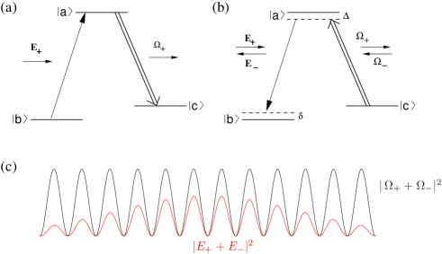
Figure 1: Level scheme for storage of light pulse $E_{+}$ by intensity reduction of control field $\Omega_{+}$ in an EIT system (a), and subsequent generation of a stationary light pulse with two counter-propagating components $E_{\pm}$ by applying two counter-propagating control fields $\Omega_{\pm}$ (b). The total field distribution of the retrieved light pulse and the control fields is indicated in (c).

A very intriguing variant of the retrieval process was suggested and experimentally demonstrated in Bajcsy-Nature-2003 . Rather than using a single coupling field, two counter-propagating retrieval beams of the same frequency and intensity were used. As indicated in fig.1b this leads to the generation of two counter-propagating probe fields $\textrm{E}_{\pm}(z,t)$ which form a quasi-stationary standing wave pattern as indicated in fig.1c. As shown in Bajcsy-Nature-2003 ; Andre-PRL-2005 the intensity profile of the retrieved field $|E_{+}+E_{-}|^{2}$ shows an interference pattern which is similar to that of the control field $|\Omega_{+}+\Omega_{-}|^{2}$. The initial envelope of this pattern is identical to the stored light field. Due to a process known as pulse matching harris93 ; Fleischhauer-PRA-1996 ; Harris-PRL-1994 , the probe-field envelope tends to approach that of the control fields with increasing time. As a consequence there is a diffusion-like behavior of the retrieved field envelope. In the following we want to theoretically analyze the underlying physics of this phenomenon within a one-dimensional model. This will then allow us to discuss a number of interesting generalizations. For this we consider the interaction Hamiltonian in a slowly-varying time frame

$$H = -\hbar\int\textrm{d}z\,\biggl{[}\Delta\sigma_{cc}(z,t)+(\delta+\Delta)\sigma_{aa}(z,t)+\Bigl{(}\Omega(z,t)\sigma_{ac}(z,t)+h.a.\Bigr{)},$$ (2)

$$\qquad\qquad+g\Bigl{(}E(z,t)\sigma_{ab}(z,t)+h.a.\Bigr{)}\biggr{]}$$

where $\Delta=\omega_{ac}-\omega_{c}$ and $\delta=\omega_{cb}-(\omega-\omega_{c})$ are the one- and two-photon detuning. The $\sigma_{\mu\nu}$’s are continuous versions of the slowly-varying (in time) single-atom flip operators

$$\sigma_{\mu\nu}(z,t)=\lim_{\Delta z\to 0}\frac{1}{\Delta z}\sum_{i\in\Delta z}\sigma_{\mu\nu}^{i}(t),\qquad\sigma_{\mu\nu}^{i}\equiv|\mu\rangle_{ii}\langle\nu|.$$ (3)

In the above sum, the atom index $i$ runs over all atoms with positions within the interval $(z-\Delta z/2,z+\Delta z/2)$. $\Omega(z,t)$ and $E(z,t)$ are the (positive-frequency) complex Rabi-frequency of the drive field and the dimensionless slowly-varying complex amplitude of the probe field respectively. Both can be decomposed into two counter-propagating contributions

$$\Omega(z,t) = \Omega_{+0}(z,t)\,{\rm e}^{ik_{c}z}+\Omega_{-0}(z,t)\,{\rm e}^{-ik_{c}z},$$ (4)

$$E(z,t) = E_{+}(z,t)\,{\rm e}^{ik_{c}z}+E_{-}(z,t)\,{\rm e}^{-ik_{c}z}.$$ (5)

Note that a fast oscillating term with the retrieve wavenumber $k_{c}$ was split off also from the probe field. Making use of the commutation relations

$$\Bigl{[}\sigma_{\alpha\beta}(z,t),\sigma_{\mu\nu}(z^{\prime},t)\Bigr{]}=\delta(z-z^{\prime})\,\Bigl{(}\delta_{\beta\mu}\,\sigma_{\alpha\nu}(z,t)-\delta_{\alpha\nu}\,\sigma_{\mu\beta}(z,t)\Bigr{)},$$ (6)

and considering the perturbative regime of a weak probe field, where we can set $\sigma_{bb}(z,t)\approx N\approx$ const., we find the following Langevin equations of motion for the atomic operators:

$$\dot{\sigma}_{ba} = -\bigl{(}i(\delta+\Delta)+\gamma\bigr{)}\sigma_{ba}+igN\left(E_{+}\textrm{e}^{ik_{c}z}+E_{-}\textrm{e}^{-ik_{c}z}\right)$$ (7)

$$+i\left(\Omega_{+0}\textrm{e}^{ik_{c}z}+\Omega_{-0}\textrm{e}^{-ik_{c}z}\right)\sigma_{bc},$$

$$\dot{\sigma}_{bc} = -i\delta\sigma_{bc}+i\left(\Omega_{+0}^{*}\textrm{e}^{-ik_{c}z}+\Omega_{-0}^{*}\textrm{e}^{ik_{c}z}\right)\sigma_{ba}.$$ (8)

We have dropped the Langevin noise operator in the equation for the optical coherence $\sigma_{ba}$ associated with the decay rate $\gamma$, since we want to work in the adiabatic limit in which this term is negligible Matsko-PRA-2001 . The above equations suggest the decomposition of the optical coherence in two counter-propagating components $\sigma_{ba}(z)=\sigma_{ba}^{(+)}(z,t)\textrm{e}^{ik_{c}z}+\sigma_{ba}^{(-)}(z,t)\textrm{e}^{-ik_{c}z}$. Substituting this into (7) and (8) and making a secular approximation, i.e. collecting terms with the similar oscillatory terms $(\textrm{e}^{\pm ik_{c}z})$ and neglecting fast oscillating contributions $(\textrm{e}^{\pm i2k_{c}z})$, yields

$$\dot{\sigma}_{ba}^{(\pm)} = -\bigl{(}i(\delta+\Delta)+\gamma\bigr{)}\sigma_{ba}^{(\pm)}+igNE_{\pm}+i\Omega_{\pm 0}\sigma_{bc},$$ (9)

$$\dot{\sigma}_{bc} = -i\delta\sigma_{bc}+i\Omega_{+0}^{*}\sigma_{ba}^{(+)}+i\Omega_{-0}^{*}\sigma_{ba}^{(-)}.$$ (10)

In the following we assume $\Omega_{\pm 0}^{*}=\Omega_{\pm 0}$. Note, that it is also possible to not make the secular approximation, as is discussed briefly in the appendix.

If the temporal changes of the slowly varying field amplitudes are slow compared to $\gamma^{-1}$, we can adiabatically eliminate the optical coherence. Under these conditions we find

$$\sigma_{ba}^{(\pm)}(z,t)=\frac{{\rm i}gNE_{\pm}(z,t)+{\rm i}\Omega_{\pm 0}(z,t)\sigma_{bc}}{i(\Delta+\delta)+\gamma},$$ (11)

which leads to the effective equation of motion for the spin coherence

$$\dot{\sigma}_{bc}=-\left(i\delta+\frac{\Omega_{0}^{2}}{i(\Delta+\delta)+\gamma}\right)\sigma_{bc}-\frac{gN\bigl{(}E_{+}\Omega_{+0}+E_{-}\Omega_{-0}\bigr{)}}{i(\Delta+\delta)+\gamma},$$ (12)

where $\Omega_{0}^{2}=\Omega_{+0}^{2}+\Omega_{-0}^{2}$. Eqs.(11,12) are the main equations for the temporal evolution of the atomic system. They describe the dynamics of the spin coherence adiabatically followed by the optical coherences. The second set of equations needed for the description of the system are the wave equations for the two probe field components $E_{\pm}$. In slowly-varying envelope approximation and within the one-dimensional model considered here, they read

$$\Bigl{(}\partial_{t}\pm c\partial_{z}\Bigr{)}\,E_{\pm}(z,t)=-i\Delta\omega\,E_{\pm}(z,t)+ig\sigma_{ba}^{(\pm)}.$$ (13)

Here $\Delta\omega=\omega-\omega_{c}$, and free-space dispersion $k=\omega/c$ and $k_{c}=\omega_{c}/c$ was assumed.

2.2 effective field equations in the adiabatic limit

In order to solve the shortened wave equations for the probe fields coupled to the atomic spins, we now apply an adiabatic perturbation to the time evolution of the atomic spin coherence, eq.(12). In lowest order of this expansion we ignore the time derivative of the spin coherence $\sigma_{bc}$ altogether. This approximation is however not sufficient, since it does not capture important effects such as the group velocity and is only valid if the characteristic pulse times are large compared to the travel time through the medium. In order to describe finite group velocities, the first order correction needs to be taken into account. This yields

$$\sigma_{bc} \approx -\frac{gN\bigl{(}E_{+}\Omega_{+0}+E_{-}\Omega_{-0}\bigr{)}}{\Omega_{0}^{2}+i\delta\Gamma}$$ (14)

$$+\frac{i(\Delta+\delta)+\gamma}{\left(\Omega_{0}^{2}+i\delta\Gamma\right)^{2}}gN\bigl{(}\Omega_{+0}\partial_{t}E_{+}+\Omega_{-0}\partial_{t}E_{-}\bigr{)},$$

where we have disregarded time derivatives of $\Omega_{\pm 0}$ and have introduced the complex parameter $\Gamma\equiv\gamma+i(\Delta+\delta)$. Substituting this result into the expression for the optical coherence $\sigma_{ba}$ and subsequently into the wave equations (13) eventually leads to the coupled field equations

$$\Bigl{(}\partial_{t}\pm c\partial_{z}\Bigr{)}\,E_{\pm} = -\left(i\Delta\omega+\frac{g^{2}N}{\Gamma}\right)\,E_{\pm}+\frac{g^{2}N\Omega_{\pm 0}\bigl{(}\Omega_{+0}\,E_{+}+\Omega_{-0}\,E_{-}\bigr{)}}{\Gamma\bigl{(}\Omega_{0}^{2}+i\delta\Gamma\bigr{)}}$$ (15)

$$-\frac{g^{2}N\Omega_{\pm 0}\bigl{(}\Omega_{+0}\,\partial_{t}E_{+}+\Omega_{-0}\,\partial_{t}E_{-}\bigr{)}}{\bigl{(}\Omega_{0}^{2}+i\delta\Gamma\bigr{)}^{2}}.$$

These equations can be written in a more transparent form by introducing the mixing angles $\theta$ and $\phi$

$$\tan^{2}\theta\equiv\frac{g^{2}N}{\Omega_{0}^{2}},\qquad\tan^{2}\phi\equiv\frac{|\Omega_{-0}|^{2}}{|\Omega_{+0}|^{2}},$$ (16)

and by assuming a small two-photon detuning, i.e. $\Omega_{0}^{2}\gg|\delta\Gamma|$:

$$\Bigl{(}\partial_{t}+c\cos^{2}\theta\partial_{z}\Bigr{)}E_{+}=-i\bigl{(}\Delta\omega\cos^{2}\theta+\delta\sin^{2}\theta\bigr{)}E_{+}$$

$$\qquad\qquad+\sin^{2}\theta\sin\phi\Bigl{(}\sin\phi\partial_{t}E_{+}-\cos\phi\partial_{t}E_{-}\Bigr{)}$$ (17)

$$\qquad\qquad-\cos^{2}\theta\frac{g^{2}N}{\Gamma}\sin\phi\bigl{(}\sin\phi E_{+}-\cos\phi E_{-}\bigr{)},$$

and

$$\Bigl{(}\partial_{t}-c\cos^{2}\theta\partial_{z}\Bigr{)}E_{-}=-i\bigl{(}\Delta\omega\cos^{2}\theta+\delta\sin^{2}\theta\bigr{)}E_{-}$$

$$\qquad\qquad-\sin^{2}\theta\cos\phi\Bigl{(}\sin\phi\partial_{t}E_{+}-\cos\phi\partial_{t}E_{-}\Bigr{)}$$ (18)

$$\qquad\qquad+\cos^{2}\theta\frac{g^{2}N}{\Gamma}\cos\phi\bigl{(}\sin\phi E_{+}-\cos\phi E_{-}\bigr{)}.$$

One recognizes that the two field components propagate with an effective group velocity $v_{\rm gr}=c\,\cos^{2}\theta$ similar to eq.(1). The first bracket on the right hand side of eqs.(17) and (18) represents a phase-mismatch, which however vanishes for a two-photon detuning chosen such that

$$\delta=-\Delta\omega\cot^{2}\theta\approx-\Delta\omega\frac{v_{\rm gr}}{c}.$$ (19)

If $|v_{\rm gr}|\ll c$ the two-photon detuning is very small and does not lead to a violation of the EIT condition. In the retrieval process the probe field will build up with a center frequency such that the phase-matching condition (19) is fulfilled.

2.3 normal modes and pulse matching

The structure of the two field equations (17) and (18) suggests the introduction of the two normal modes Harris-PRL-1994

$$E_{S}\equiv\cos\phi\,E_{+}+\sin\phi\,E_{-},\qquad E_{D}\equiv\sin\phi\,E_{+}-\cos\phi\,E_{-},$$ (20)

which we denote as sum and difference normal mode. In terms of these modes the propagation equations read

$$\Bigl{(}\partial_{t}+v_{\rm gr}\cos(2\phi)\partial_{z}\Bigr{)}\,E_{S}+v_{\rm gr}\sin(2\phi)\partial_{z}\,E_{D}=$$

$$\qquad\qquad\qquad+v_{\rm gr}\bigl{(}\partial_{z}\phi\bigr{)}\bigl{(}\sin(2\phi)E_{S}-\cos(2\phi)E_{D}\bigr{)},$$ (21)

$$\Bigl{(}\partial_{t}-c\cos(2\phi)\partial_{z}\Bigr{)}\,E_{D}+c\sin(2\phi)\partial_{z}\,E_{S}=-\frac{g^{2}N}{\Gamma}E_{D}$$

$$\qquad\qquad\qquad-c\bigl{(}\partial_{z}\phi\bigr{)}\bigl{(}\cos(2\phi)E_{S}+\sin(2\phi)E_{D}\bigr{)}.$$ (22)

Here we have assumed that the mixing angles $\theta$ and $\phi$ can be space dependent but are constant in time. At the same time, in lowest order of the adiabatic expansion, the atomic spin coherence follows the evolution of the sum normal mode $E_{S}$, hence we find from eq.(14)

$$\sigma_{bc}=-\sqrt{N}\tan\theta\,E_{S}.$$ (23)

One recognizes from (21) and (22) that apart from the coupling between the normal modes $E_{S}$ and $E_{D}$, the difference mode $E_{D}$ is strongly absorbed due to the term $g^{2}N/\Gamma$ on the right hand side. As a consequence the amplitudes of the retrieved fields approach a configuration where $E_{D}\rightarrow 0$, i.e. a configuration where the probe amplitudes match those of the drive fields:

$$\frac{E_{+}}{E_{-}}\rightarrow\cot\phi=\frac{\Omega_{+}}{\Omega_{-}}.$$ (24)

This phenomenon called pulse-matching is well-known for EIT systems harris93 ; Harris-PRL-1994 ; Fleischhauer-PRA-1996 .

One recognizes that for almost identical control fields, i. e. $\Omega_{+}\approx\Omega_{-}$ the group velocity of the sum mode $E_{S}$ and difference mode $E_{D}$ are very small due to the $\cos(2\phi)$-term. It is zero if the strength of the two counter-propagating control beams is exactly the same. If $\Omega_{+}$ is bigger than $\Omega_{-}$ the sum mode moves to the $+z$ direction and vice versa. Finally even if the ratio of the control field envelopes is spatially constant, i.e. if $\partial_{z}\phi=0$, a small amplitude of the difference mode will be generated out of the sum mode due to the term proportional to $\partial_{z}E_{S}$ until $E_{S}$ is constant in space. This coupling will give rise to the slow spatio-temporal evolution discussed in the following sections.

3 Quasi-stationary pulses of light from spatially homogeneous retrieval beams

Let us first consider the case of two spatially homogeneous control fields with equal intensity, i.e.

$$\cos(2\phi)=0,\qquad\partial_{z}\phi=0.$$ (25)

This can be realized e.g. by two laser beams of the same intensity with a negligible curvature of the phase fronts, i. e. in the plain wave regime. In this case the propagation equations for the sum and difference mode (21) and (22) simplify to

$$\partial_{t}E_{S} = -v_{\rm gr}\partial_{z}E_{D},$$ (26)

$$\partial_{t}E_{D} = -c\partial_{z}E_{S}-\frac{g^{2}N}{\Gamma}E_{D}.$$ (27)

3.1 Adiabatic elimination of difference normal mode and diffusion equation for resonant probe fields

Let us consider the case where the drive field detuning $\Delta$ is chosen such that the probe fields are resonant, i.e. $\Delta+\delta=0$. Since for an optically dense medium the phase matching condition (19) requires only a very small two-photon detuning, this is essentially equivalent to the case of resonant drive fields. Then $\Gamma=\gamma+i(\Delta+\delta)=\gamma$ and eq.(27) shows that the difference normal mode is damped with a rate $g^{2}N/\gamma=c/l_{\rm abs}$, where $l_{\rm abs}$ is the absorption length of the medium in the absence of EIT. For a medium with sufficiently high optical density $OD=l/l_{\rm abs}$ the absorption length is typically on the mm scale and thus the decay time is on the order of a few picoseconds. The typical pulse times in light storage experiments are however much larger. Thus an adiabatic elimination of the difference normal mode, i.e. neglecting $\partial_{t}E_{D}$ as compared to $(g^{2}N/\gamma)E_{D}$, seems justified. Such an elimination leads to

$$E_{D}=-l_{\rm abs}\frac{\partial}{\partial z}E_{S}.$$ (28)

Making use of this approximation we find for the sum normal mode $E_{S}$ a simple diffusion equation

$$\frac{\partial}{\partial t}E_{S}=v_{\rm gr}l_{\rm abs}\,\frac{\partial^{2}}{\partial z^{2}}E_{S}=D\,\frac{\partial^{2}}{\partial z^{2}}E_{S}.$$ (29)

In the retrieval process two counter-propagating probe field components are created with an initial envelope given by the stored spin excitation. These components then undergo a diffusion process with a diffusion constant $D=v_{\rm gr}l_{\rm abs}$ given by the product of group velocity and absorption length. This is illustrated in fig.2 where false-color images show the two field distributions $E_{+}(z,t)$ and $E_{-}(z,t)$ for a storage process followed by a partial retrieve with two homogeneous, counter-propagating drive beams of equal amplitude. The data are obtained from a numerical solution of the wave equation (13) as well as the full set of atomic density matrix equations in secular approximation. The predicted diffusive behavior is nicely reproduced.

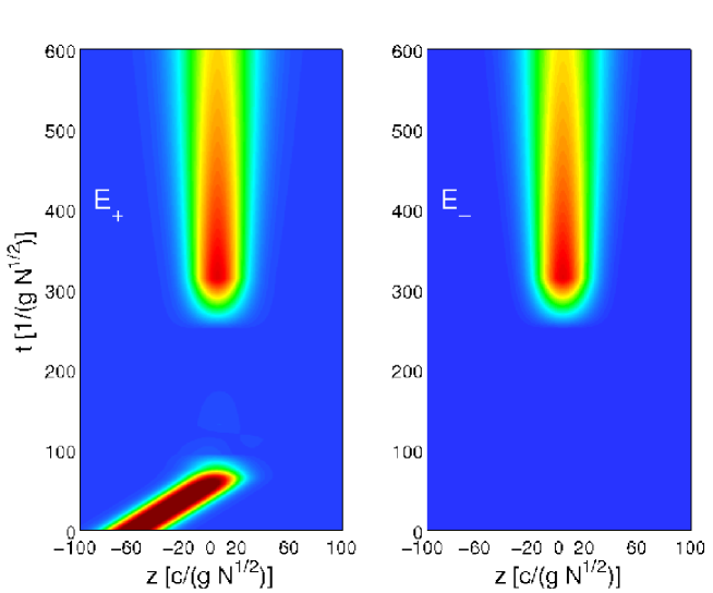
Figure 2: Numerical simulation of storage and partial retrieval of a light pulse, where in the retrieval process two counter-propagating drive beams with equal and spatially homogeneous intensities have been applied. For the storage and retrieval we have used $\cos^{2}\theta_{+}=0.5*[1-\tanh(0.1*(t-65))]+0.5*1/3*[1+\tanh(0.1*(t-300))]$, where $\tan^{2}\theta_{\pm}=g^{2}N/\Omega_{\pm 0}^{2}$. For $\cos^{2}\theta_{-}$ only the second term was used. The color code represents the amplitude of the forward ($E_{+}$) and backward ($E_{-}$) propagating components of the probe field. The parameters used for the numerical simulation are: $\delta=\Delta=\Delta\omega=0$ and $\gamma=1$ and the initial width of the Gaussian wave-packet was $\Delta z(t=0)=10$.

In the diffusion process the width of the probe field distribution as well as that of the collective spin excitation (see eq.(23)) increase according to

$$\Delta z^{2}(t)=\Delta z^{2}(t_{0})+2D(t-t_{0}).$$ (30)

Associated with this is a decrease of the excitation density. Since in a diffusion process the spatial integral of the field is constant but not the integral of the square of the field, representing the number of photons, there is also a (non-exponential) decay of the total number of excitations. After the control fields are switched on again, the sum mode has a Gaussian shape with width $\Delta z(0)$, and the total excitation, i.e. in the retrieved fields and the collective spin, evolves according to

$$n_{\rm tot}(t)=n_{\rm tot}(0)\frac{\Delta z(0)}{\sqrt{\Delta z^{2}(0)+2Dt}}.$$ (31)

Thus in order to have negligible losses, the time over which a stationary pulse can be maintained is limited by

$$t\ll\frac{\Delta z^{2}(0)}{D}=\frac{\Delta z^{2}(0)}{v_{\rm gr}l_{\rm abs}},$$ (32)

which is exactly the characteristic time for the spread of the initial wave-packet.

3.2 Small optical depth

If the optical depth of the medium is small, the adiabatic elimination of $E_{D}$ may be no longer justified. It is still possible however to find analytic results for the moments of the stationary light field. First of all one finds from eqs.(26) and (27) that like in the diffusion limit discussed above, the integral of $E_{S}$ is a constant of motion since $E_{D}(z=\pm\infty)=0$:

$$\frac{{\rm d}}{{\rm d}t}A(t)=\frac{{\rm d}}{{\rm d}t}\int_{-\infty}^{\infty}\!\!{\rm d}z\,E_{S}(z,t)=0.$$ (33)

Assuming an initially symmetric spin excitation around $z=0$, the width of the retrieved light beam is given by the second moment of the sum mode $d(t)\equiv\Delta z^{2}(t)=\int_{-\infty}^{\infty}\,{\rm d}z\,z^{2}\,E_{S}(z,t)/A$, which is coupled to the first moment of the difference mode $g(t)\equiv\int_{-\infty}^{\infty}\,{\rm d}z\,z\,E_{D}(z,t)/A$:

$$\frac{{\rm d}}{{\rm d}t}d(t) = 2v_{\rm gr}g(t),$$ (34)

$$\frac{{\rm d}}{{\rm d}t}g(t) = -\frac{c}{l_{\rm abs}}g(t)+c.$$ (35)

The solution of these equations can easily be found and reads

$$d(t)=d(0)+2Dt+2D\frac{l_{\rm abs}}{c}\left(1-\frac{g(0)}{l_{\rm abs}}\right)\left({\rm e}^{-ct/l_{\rm abs}}-1\right).$$ (36)

One recognizes that a small absorption length $l_{\rm abs}$ only affects the short-time evolution. In fig.3 a comparison between the analytical prediction for $\delta(t)$ obtained from eq.(36) with $v_{\rm gr}\to v_{\rm gr}(t)$ and a numerical simulation of the Maxwell-Bloch equations is shown. Apart from a short initial time period, where due to the time dependence of $v_{\rm gr}(t)$ non-adiabatic couplings lead to small deviations, there is a nearly perfect agreement between analytic prediction and numerical simulation.

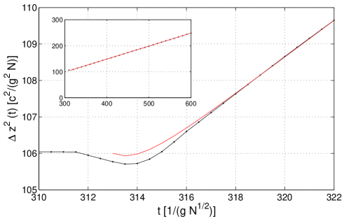
Figure 3: Comparison between analytic prediction for $\Delta z^{2}(t)$ of the stationary wave-packet of light from eq.(36) with a numerical simulation of the coupled Maxwell-Bloch equations. The data are based on the simulation of fig.2. The insert shows the behavior on a larger time scale.

3.3 Non-equal but constant drive intensities

If the intensities of the counter-propagating retrieve beams are not equal but constant in time and space, one has

$$\cos(2\phi)\neq 0,\qquad\partial_{z}\phi=0.$$ (37)

As a consequence the equation of motion of the sum normal mode attains, after adiabatic elimination of the difference mode, a finite drift term

$$\Bigl{(}\partial_{t}+v_{\rm gr}\cos(2\phi)\partial_{z}\Bigr{)}\,E_{S}=v_{\rm gr}l_{\rm abs}\sin^{2}(2\phi)\,\partial_{z}^{2}E_{S}.$$ (38)

Transforming into a moving frame with $z^{\prime}=z-v_{\rm gr}\cos(2\phi)t$ and $t^{\prime}=t$ leads again to a diffusion equation with a modified diffusion constant $\tilde{D}=v_{\rm gr}l_{\rm abs}\sin^{2}(2\phi)$. Thus in the case of non equal, but constant drive intensities, the diffusive behavior of the quasi-stationary light is superimposed by a drift motion with a small velocity $v_{\rm gr}\cos(2\phi)$. This can be understood in a very intuitive way. If one of the drive fields is stronger than the other one, Raman scattering occurs with higher probability into the probe mode co-propagating with the stronger drive field which causes a drift motion of the quasi-stationary wave-packet.

4 Stationary pulses of light generated by spatially modulated retrieve fields

In this section, we discuss two techniques to manipulate the shape of stationary pulses with the ultimate goal of confining the pulse to very short spatial dimensions. Initially the pulse is stored as a spin coherence with a spatial envelope that extends over many wavelengths. We have seen in the previous sections that the (partial) retrieval of the stored light pulse by counter-propagating control fields leads to quasi-stationary pulses of light. The shape of these stationary pulses is determined by the envelope of the initial spin coherence as well as the control-field envelopes through the mechanism of pulse-matching.

This suggests two different mechanisms to manipulate the shape of the stationary pulse of light. In the first method the atoms are illuminated by a frequency comb, i.e. with control beams that have multiple frequency components of equal intensity in the forward and backward direction. In this way many corresponding frequency components are generated for the signal field. These components interfere to create a very sharp spatial envelope, which is matched to the sharp spatial envelope of the control field, potentially confined over only a few wavelengths (see Fig. 4).

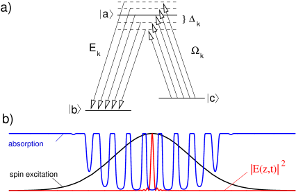
Figure 4: (a) Atomic level structure with multiple-frequency-component control field $\Omega(z,t)=\sum_{k}\Omega_{k}e^{-i\Delta_{k}(t-z/c)}$, and generated signal field $E(z,t)=\sum_{k}{E}_{k}(z,t)e^{-i\Delta_{k}(t-z/c)}$. (b) Generated signal field envelope, showing tight localization due to constructively interfering frequency components (frequency comb).

A second method employs a spatial modulation in the difference of the forward and backward retrieve intensities. In the last section we have seen that unequal retrieve intensities can lead to a drift motion of the stationary field with an effective group velocity $v_{\rm gr}\cos(2\phi)$. If e.g. $v_{\rm gr}\cos(2\phi)$ would be negative for positive values of $z$ and positive for negative values of $z$, the associated drift motion would tend to spatially compress the stationary field. As will be shown this can compensate the diffusive spread found in the last section. This situation, indicated in fig. 5, can be achieved when $\phi$ (and in general also $\theta$) are made $z$ dependent.

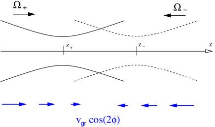
Figure 5: Paraxial retrieve lasers with spatially varying, Gaussian intensity profiles determined by the position of the focal points $z_{+}\neq z_{-}$ create a spatially varying effective group velocity.

4.1 Shaping of stationary light pulses using the optical comb technique

Let us first consider the case when the atomic sample is irradiated with several counter-propagating control fields, with detunings $\Delta_{k}$, and (complex) Rabi frequencies $\Omega_{\pm k}$, such that the slowly-varying total Rabi frequency reads $\Omega(z,t)=\sum_{k}\left(\Omega_{+k}{\rm e}^{-i\Delta_{k}(t+z/c)}+\Omega_{-k}{\rm e}^{-i\Delta_{k}(t-z/c)}\right)$. $\Delta_{k}=\omega_{k}-\omega_{ab}$ is the detuning from the atomic resonance. For simplicity we here consider a degenerate level scheme, i.e. $\omega_{ab}=\omega_{ac}$. We assume equal intensities of the corresponding forward and backward components $|\Omega_{+k}|=|\Omega_{-k}|$. Corresponding to these driving fields are signal field slowly varying amplitudes ${E}_{\pm k}(z,t)$, so that the total signal field envelope is $E(z,t)=\sum_{k}\left({E}_{+k}(z,t){\rm e}^{-i\Delta_{k}(t-z/c)}+{E}_{-k}(z,t){\rm e}^{-i\Delta_{k}(t+z/c)}\right)$.

Assuming $|\Delta_{k\neq 0}|\gg|\Omega_{k\neq 0}|$ so that we can ignore coupling of the frequency components through off-resonant processes, we may also expand the optical polarization as $\sigma_{ba}(z,t)=\sum_{k}\left(\sigma_{ba}^{(+k)}(z,t){\rm e}^{-i\Delta_{k}(t-z/c)}+\sigma_{ba}^{(-k)}(z,t){\rm e}^{-i\Delta_{k}(t+z/c)}\right)$. Within the weak-probe and secular approximation and assuming two-photon resonance of all associated pairs of fields we obtain the following equations of motion

$$\dot{\sigma}_{ba}^{(\pm k)} = -\bigl{(}i\Delta_{k}+\gamma\bigr{)}\sigma_{ba}^{(\pm k)}+igNE_{\pm k}+i\Omega_{\pm k}\sigma_{bc},$$ (39)

$$\dot{\sigma}_{bc} = +\sum_{k}\left[i\Omega_{+k}^{*}\sigma_{ba}^{(+k)}+i\Omega_{-k}^{*}\sigma_{ba}^{(-k)}\right].$$ (40)

Here again the Langevin noise operators associated with the spontaneous decay from the excited state in eqs.(39) have been neglected as they do not contribute in the adiabatic limit. The atomic polarizations $\sigma_{ba}^{(\pm k)}$ drive the probe field components $E_{\pm k}$ through the shortened one-dimensional wave equations

$$\Bigl{(}\partial_{t}\pm c\partial_{z}\Bigr{)}\,E_{\pm k}(z,t)=ig\sigma_{ba}^{(\pm k)}.$$ (41)

Solving eq.(39) adiabatically for $\sigma_{ba}^{(\pm k)}$ yields

$$\sigma_{ba}^{(\pm k)}=\frac{igN}{\Gamma_{k}}E_{\pm k}+\frac{i\Omega_{\pm k}}{\Gamma_{k}}\sigma_{bc},$$ (42)

where we have introduced the notation $\Gamma_{k}=\gamma+i\Delta_{k}$. Substituting this result into eq.(40) for the ground-state coherence leads to

$$\dot{\sigma}_{bc}=-\sum_{k}\frac{|\Omega_{+k}|^{2}+|\Omega_{-k}|^{2}}{\Gamma_{k}}\sigma_{bc}-gN\sum_{k}\frac{\Omega_{+k}^{*}E_{+k}+\Omega_{-k}^{*}E_{-k}}{\Gamma_{k}}.$$ (43)

Letting $\Delta_{0}=0$ and $|\Delta_{k\neq 0}|\gg\gamma,|\Omega_{\pm k}|$, we find that the spin coherence is driven only by the resonant fields, i.e.

$$\dot{\sigma}_{bc}\approx-\frac{\Omega_{0}^{2}}{\gamma}\sigma_{bc}-gN\frac{\Omega_{+0}^{*}E_{+0}+\Omega_{-0}^{*}E_{-0}}{\gamma},$$ (44)

where $\Omega_{0}^{2}=|\Omega_{+0}|^{2}+|\Omega_{-0}|^{2}$. In a similar way as in Sec.2.2 we can solve this equation in first order of an adiabatic expansion. This yields

$$\sigma_{bc}=-gN\frac{E_{+0}\Omega_{+0}^{*}+E_{-0}\Omega_{-0}^{*}}{\Omega_{0}^{2}}+\frac{\gamma}{\Omega_{0}^{4}}gN\Bigl{(}\Omega_{+0}^{*}\partial_{t}E_{+0}+\Omega_{-0}\partial_{t}E_{-0}\Bigr{)}.$$ (45)

Substituting this result first into the equations for the resonant fields $E_{\pm 0}$ leads to similar equations as in Sec.2.

$$\Bigl{(}\partial_{t}\pm c\cos^{2}\theta\partial_{z}\Bigr{)}E_{\pm 0}=\pm\frac{\sin^{2}\theta}{\Omega_{0}^{2}}\Omega_{\mp 0}^{*}\bigl{(}\Omega_{-0}\partial_{t}E_{+0}-\Omega_{+0}\partial_{t}E_{-0}\bigr{)}$$ (46)

$$\qquad\qquad\mp\cos^{2}\theta\frac{g^{2}N}{\Omega_{0}^{2}\gamma}\Omega_{\mp 0}^{*}\bigl{(}\Omega_{-0}E_{+0}-\Omega_{+0}E_{-0}\bigr{)}.$$

Taking into account that $|\Omega_{-k}|=|\Omega_{+k}|$ these equations can be written in a simpler form introducing sum and difference normal modes $E_{S}=(\Omega_{+0}^{*}E_{+0}+\Omega_{-0}^{*}E_{-0})/\Omega_{0},$ $E_{D}=(\Omega_{-0}E_{+0}-\Omega_{+0}E_{-0})/\Omega_{0}$:

$$\partial_{t}E_{S} = -v_{\rm gr}\partial_{z}E_{D},$$ (47)

$$\partial_{t}E_{D} = -c\partial_{z}E_{S}-\frac{g^{2}N}{\gamma}E_{D}.$$ (48)

The second term on the right hand side of eq.(48) leads to a fast decay of the difference mode, such that in the long-time limit the resonant probe-field amplitudes are matched to the corresponding drive-field amplitudes

$$\Omega_{-0}E_{+0}=\Omega_{+0}E_{-0}=-\frac{\Omega_{-0}\Omega_{+0}}{gN}\sigma_{bc}.$$ (49)

As in section 2, the sum normal mode undergoes a diffusion process under conditions when the difference normal mode can be adiabatically eliminated. As a consequence the spin excitation, which adiabatically follows the sum normal mode, does the same, i.e.

$$\partial_{t}\sigma_{bc}(z,t)=D\partial_{z}^{2}\sigma_{bc}(z,t),$$ (50)

with $D=v_{\rm gr}l_{\rm abs}$.

For the non-resonant probe-field components $E_{\pm k}$, $k\neq 0$ one finds the shortened wave-equations

$$\Bigl{(}\partial_{t}\pm c\partial_{z}\Bigr{)}\,E_{\pm k}(z,t)=-\frac{g^{2}N}{\Gamma_{k}}E_{\pm k}-\frac{g\Omega_{\pm k}}{\Gamma_{k}}\sigma_{bc}.$$ (51)

The second term on the right hand side does not depend on $E_{\pm k}$. As a consequence, assuming a sufficiently dense medium, the off-resonant probe amplitude may be adiabatically eliminated leading to

$$E_{\pm k}=-\frac{\Omega_{\pm k}}{gN}\sigma_{bc}.$$ (52)

Noting that a similar relation holds for the resonant components in the long-time limit, eq.(49), we finally arrive at

$$E(z,t) = \sum_{k}\left(E_{+k}(z,t){\rm e}^{-i\Delta_{k}(t-z/c)}+E_{-k}(z,t){\rm e}^{-i\Delta_{k}(t+z/c)}\right)$$

$$= -\sum_{k}\left(\Omega_{+k}{\rm e}^{-i\Delta_{k}(t-z/c)}+\Omega_{-k}{\rm e}^{-i\Delta_{k}(t+z/c)}\right)\frac{\sigma_{bc}(z,t)}{gN},$$

$$= -\Omega(z,t)\frac{\sigma_{bc}(z,t)}{gN}.$$

Thus the electric field envelope $E(z,t)$ becomes matched to the control field envelope $\Omega(z,t)$ modified by the spin coherence $\sigma_{bc}(z,t)$. This allows to control the stationary pulse shape through control of the retrieve amplitudes and phases.

Note that the condition for this analysis to hold is $l_{\rm spin}/l_{\rm abs}\gg$ max$\{\Delta_{k}\}/\gamma$. Taking the length of the initial spin excitation $l_{\rm spin}$ to be such that the pulse just fits inside the medium $l_{\rm spin}\sim l$, this condition implies that the maximum frequency detuning $\Delta_{max}$ for which the stationary pulse can adiabatically follow the control field through pulse matching, is given by $\Delta_{max}\sim\gamma\,OD$, where $OD=\frac{g^{2}Nl}{\gamma c}=l/l_{\rm abs}$ is the on-resonance optical depth. Thus spatial features as small as the optical depth can be imposed on the stationary pulse through the frequency comb technique.

It should be noted, however, that the generation of spatially narrow stationary fields by means of the frequency-comb technique is a filtering process rather than a compression of excitation. In fact the total number of probe photons created by a frequency comb is much less than in the case when only the resonant components $\Omega_{\pm 0}$ of the retrieve laser are present. The excitation density at the center of the stationary photon wavepacket is the same in both cases, while in the wings it is substantially smaller for the case of the frequency comb as compared to the case of homogeneous retrieve beams.

4.2 Shaping of stationary light pulses using a spatially varying group velocity

Let us now discuss the second method indicated in fig. 5 in detail. Assuming again single and two-photon resonance and an optically thick medium, we can adiabatically eliminate the difference normal mode from (22). This yields

$$E_{D}\approx-\sin(2\phi)l_{\rm abs}\partial_{z}E_{S}-\cos(2\phi)l_{\rm abs}\left(\partial_{z}\phi\right)\,E_{S},$$ (54)

where we have assumed that $\phi$ changes only little over the absorption length $l_{\rm abs}$ and thus $|(g^{2}N/\gamma)|\gg|(\partial_{z}\phi)\sin(2\phi)|$. Substituting this into (21) gives

$$\frac{\partial}{\partial t}E_{S}=A_{0}\,E_{S}+\frac{\partial}{\partial z}\Bigl{[}A_{1}\,E_{S}\Bigr{]}+\frac{\partial^{2}}{\partial z^{2}}\Bigl{[}D\,E_{S}\Bigr{]},$$ (55)

where $D=v_{\rm gr}l_{\rm abs}$ is the diffusion constant introduced before, and the coefficients $A_{0}$ and $A_{1}$ read

$$A_{0} = -v_{\rm gr}\bigl{[}(\partial_{z}\phi)\sin(2\phi)+2l_{\rm abs}(\partial_{z}\phi)^{2}\sin^{2}(2\phi)$$ (56)

$$\qquad-l_{\rm abs}(\partial_{z}\phi)^{2}\cos^{2}(2\phi)-(\partial^{2}_{z}\phi)\cos(2\phi)\sin(2\phi)\bigr{]},$$

$$A_{1} = -v_{\rm gr}\bigl{[}1+4l_{\rm abs}(\partial_{z}\phi)\bigr{]}.$$ (57)

The constant term proportional to $A_{0}$ in eq.(55) can be removed by the substitution

$$E_{S}=\widetilde{E}_{S}\,\exp\bigl{\{}A_{0}t\bigr{\}},$$ (58)

which results into a Fokker-Planck equation for $\widetilde{E}_{S}$:

$$\frac{\partial}{\partial t}\widetilde{E}_{S}=\frac{\partial}{\partial z}\Bigl{[}A_{1}\,\widetilde{E}_{S}\Bigr{]}+\frac{\partial^{2}}{\partial z^{2}}\Bigl{[}D\,\widetilde{E}_{S}\Bigr{]}.$$ (59)

In the following we will discuss the spatio-temporal evolution of $E_{S}$ resulting from this equation.

Non equal drive fields lead to an effective group velocity $v_{\rm gr}\cos(2\phi)$ for the sum normal mode. If this group velocity is tailored in such a way that it is negative for positive values of $z$ and positive for negative values of $z$, there is an effective drift towards the origin. This force may compensate the dispersion due to the absorption of large-$k$ components of the probe field found in section 3. We thus consider as the simplest example the special case of a linearly varying intensity difference of the two drive fields with a constant sum $\Omega_{0}^{2}=$ const.:

$$\cos(2\phi)=\frac{|\Omega_{+}|^{2}-|\Omega_{-}|^{2}}{\Omega_{0}^{2}}\approx-\frac{z}{l},\qquad\sin(2\phi)\approx 1\,.$$ (60)

This situation is realized e.g. if the two control fields are paraxial, Gaussian laser beams with focal points at $z_{\pm}\approx\pm 2l$.

Figure 6: The prefactor of the drift term for the configuration of to separated Gaussian beams. The focal points of the two beams are located at $z_{\pm}=\pm 20\,l_{\rm abs}$. The linear regime under consideration in this section is clearly visible.

The linear approximation is of course only valid for $|z|\ll l$. In this case eq.(59) turns into the Fokker-Planck equation of the Ornstein-Uhlenbeck process Gardiner-Handbook for which exact analytic solutions are known

$$\frac{\partial}{\partial t}\widetilde{E}_{S}=\frac{\partial}{\partial z}\Bigl{[}\,v_{\rm gr}\frac{z}{l}\widetilde{E}_{S}\Bigr{]}+\frac{\partial^{2}}{\partial z^{2}}\Bigl{[}D\,\widetilde{E}_{S}\Bigr{]}.$$ (61)

Here we have neglected contributions proportional to $l_{\rm abs}/l$ as compared to unity. The Ornstein-Uhlenbeck process has a stationary Gaussian solution with width $\sqrt{l\,l_{\rm abs}}$. Noting that now $A_{0}=-v_{\rm gr}(\partial_{z}\phi)=-v_{\rm gr}/2l$ this gives with eq.(58) in the long-time limit:

$$E_{S}(z,t)=\widetilde{E}_{S}(z)\,\exp\bigl{\{}A_{0}t\bigr{\}}\longrightarrow\exp\left\{-\frac{z^{2}}{{2}ll_{\rm abs}}\right\}\exp\left\{-\frac{v_{\rm gr}t}{2l}\right\}.$$ (62)

The use of retrieve lasers with non-equal and spatially varying intensities thus acts like an effective cavity for the probe field with a ring-down time $l/v_{\rm gr}$ given by the time a photon travels between the intensity maxima of the two drive lasers.

The initial-value problem of the Ornstein-Uhlenbeck process can be solved by making use of the eigensolutions $\{\Phi_{n}(z),\lambda_{n}\}$ of the corresponding backward equation Gardiner-Handbook

$$\frac{\partial^{2}}{\partial z^{2}}\,\Phi_{n}(z)-\frac{v_{\rm gr}}{D}\frac{z}{l}\frac{\partial}{\partial z}\,\Phi_{n}(z)+\frac{\lambda_{n}}{D}\,\Phi_{n}(z)=0.$$ (63)

Eq.(63) is the differential equation of the Hermite polynomials $H_{n}$ and thus the eigenvalues $\lambda_{n}$ and eigenfunctions $\Phi_{n}(z)$ read

$$\lambda_{n} = n\,\frac{v_{\rm gr}}{l},\qquad\qquad n\in\{0,1,2,\dots\},$$ (64)

$$\Phi_{n}(z) = (2^{n}n!)^{-1/2}\,H_{n}\Bigl{(}\frac{z}{\sqrt{2l\,l_{\rm abs}}}\Bigr{)}.$$ (65)

The general solution of the initial value problem then reads

$$E_{S}(z,t)=\sum_{n=0}^{\infty}\frac{c_{n}}{\sqrt{2^{n+1}n!\pi\,l\,l_{\rm abs}}}\,\exp\left\{-\frac{z^{2}}{2\,l\,l_{\rm abs}}\right\}\times$$

$$\qquad\qquad\quad\times\,H_{n}\Bigl{(}\frac{z}{\sqrt{2\,l\,l_{\rm abs}}}\Bigr{)}\,\exp\left\{-\frac{v_{\rm gr}(n+1/2)t}{l}\right\}.$$ (66)

The coefficients $c_{n}$ are determined by the initial field $E_{S}(z,0)$:

$$c_{n}=\int_{-\infty}^{\infty}\!\!{\rm d}z\,E_{S}(z,0)\,H_{n}\Bigl{(}\frac{z}{\sqrt{2\,l\,l_{\rm abs}}}\Bigr{)}\,(2^{n}n!)^{-1/2}.$$ (67)

It is interesting to note that, apart from the additional overall damping term, eq.(66) is very similar to a damped harmonic oscillator with oscillator length $\sqrt{l\,l_{\rm abs}}$. If the stored light pulse is a Gaussian and if the separation of the foci of the two retrieve lasers is chosen such that the width of the stored light pulse is less than the effective oscillator length $\sqrt{l\,l_{\rm abs}}$, only the fundamental mode $\Phi_{0}$ gets excited in the retrieve process. In this case a spatially constant field distribution is created. The field has however a finite lifetime determined by the decay rate $\gamma_{\rm eff}=v_{\rm gr}/l$. As a consequence the total excitation decays in time according to

$$n_{\rm tot}(t)=n_{\rm tot}(0)\,\exp\bigl{\{}-v_{\rm gr}t/l\bigr{\}}.$$ (68)

In order to have negligible losses, the time over which the stationary pulse can be maintained is limited by exactly the same expression as in the diffusion case

$$t\ll\frac{l}{v_{\rm gr}}=\frac{\Delta z^{2}(0)}{v_{\rm gr}l_{\rm abs}}.$$ (69)

If the separation of the focal points in the retrieve process is much smaller than $l_{\rm spin}^{2}/l_{\rm abs}$ the generated stationary light pulse has a much narrower width than the original spin excitation ($l_{\rm spin}$). In this case a large number of higher-order Gauss-Hermite modes is excited however (see eq.(67)), which decay much faster than the fundamental mode. Thus as in the case of the frequency comb very narrow spatial distributions of the stationary field can be created, however only through a filter process.

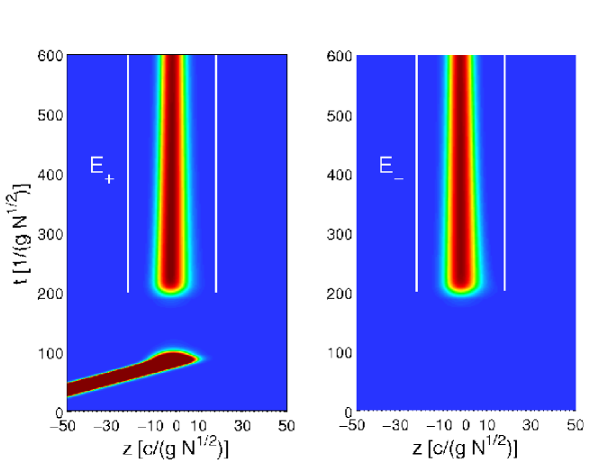
Figure 7: Storage of a Gaussian pulse and subsequent retrieval with two control beams with spatially changing intensity difference. The maxima of the intensities of $\Omega_{\pm}$ are indicated by the two white lines. Close to the midpoint between these lines the normalized intensity difference $(|\Omega_{+0}|^{2}-|\Omega_{-0}|^{2})/\Omega_{0}^{2}$ varies linearly with $z$. The generation of fields with constant spatial shape is apparent. The parameters are that of fig.(2). In addition Gaussian beam profiles $\Omega_{\pm}(z)=1/w_{\pm}(z)$ with $w_{\pm}(z)=\sqrt{1-2(z-z_{\pm})/\pi}$ have been assumed.

In fig.7 a numerical simulation of the the retrieval using two control beams with separated foci is shown. Initially a Gaussian probe pulse is stored in a collective spin excitation. The center of the stored probe pulse is in the middle between the two foci, indicated by the two white lines and the width of the pulse is on the order of $\sqrt{l\,l_{\rm abs}}$. Thus mainly the fundamental mode $\Phi_{0}$ is excited, which can be seen from the constant spatial shape of the retrieved wave-packet.

5 Spatial compression of stationary pulses of light

We have seen in the last section that the use of retrieve lasers with spatially modulated intensities does allow the generation of stationary light pulses with very narrow spatial shapes. The underlying process is however a filter process and thus accompanied either by reduction of the photonic component in the polariton or by large losses. Nevertheless both techniques open interesting possibilities for the spatial compression of a stored photon with small losses. If a stationary light pulse is created e.g. with separated foci of the drive lasers as explained in the previous section, and the distance between the focal points is reduced as a function of time in an adiabatic way, the spatial width of the stationary pulse follows. This results in a spatial compression of the probe excitation. As the effective decay rate of a stationary pulse $\gamma_{\rm eff}$ increases with decreasing pulse width, the control fields should be switched off immediately after the compression. Fig. 8 shows a numerical example for such a process. After retrieval of a stored pulse with separated foci, whose position is indicated by white lines, the distance between the focal points is reduced. One can see very clearly that the field density as well as the density of the spin excitation is substantially increased in this process. This suggests that by changing the spatial profile of the control field in time, either using the optical comb technique or displaced foci, spatial compression can be achieved.

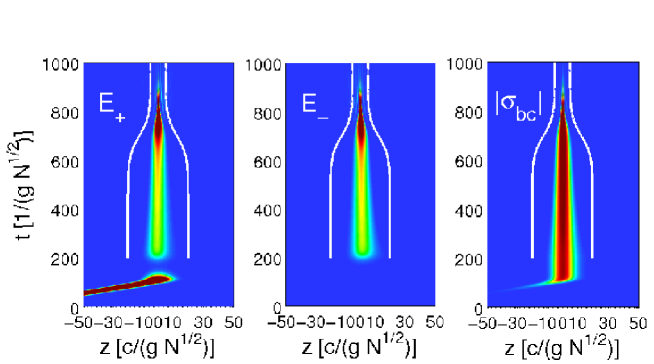
Figure 8: Retrieval of a stored pulse and spin excitation using drive fields with separated foci and subsequent reduction of their separation. The position of the focal points is indicated by white lines. One clearly recognizes a compression of the probe field associated with an increase of the field density. The parameters are the same as in fig.(7) except for $\gamma=0.05$. The foci move like: $z_{\pm}(t)=20\mp 10*0.5*[1+\tanh(0.0125*(t-700))]$

.

In fig.9 the temporal evolution of the peak density and the total excitation (i.e. photon number of the stationary field plus spin excitations in the atomic ensemble) are shown for the example of fig.8. One recognizes that when the peak density increases the total number of excitations starts to decrease very rapidly. Clearly an optimization is needed to maximize fidelity and compression. In order to find optimum conditions and to estimate the maximum possible compression from the theoretical model, it is necessary to include non-adiabatic couplings into the description. Finally, it is not clear if spatial compression of this kind can be used to enhance further nonlinear optical processes using the techniques of Ref. Andre-PRL-2005 . This analysis is beyond the scope of the present paper and will be discussed in detail elsewhere.

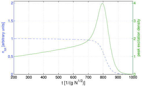
Figure 9: Peak excitation density (solid line) and total excitation (dashed line) as function of time for the example of fig.8. All quantities are normalized to their value at $t=200(g\sqrt{N})^{-1}$.

6 Summary and outlook

In the present paper we have discussed the generation and coherent control of stationary pulses of light by storage of a light pulse in a collective spin excitation via EIT and subsequent partial retrieval of this excitation with counter-propagating retrieve lasers. We have shown that for equal and spatially homogeneous intensities of the forward and backward retrieve beams a quasi-stationary wavepacket of the probe light is generated with an initial envelope given by the spin excitation. For an optically thick medium the dynamics of the wavepacket is described by a diffusion equation with a diffusion constant given by the product of group velocity and absorption length without EIT. The physical mechanisms for the diffusion of the stationary pulse is the well-known phenomenon of pulse matching of probe and retrieve field components in EIT. We have shown furthermore that spatially modulated retrieve lasers can be used to manipulate the shape of the stationary light pulse and in particular to spatially compress the excitation. Making use of a frequency comb for the retrieve fields a very narrow spatial distribution of the probe field can be generated. Likewise the use of retrieve fields with spatially varying intensity difference can lead to a narrow non-dispersing but exponentially decaying field distribution. In both cases the narrow field distribution is however created by a filtering process. Thus these techniques can not straightforwardly be applied, e.g. to applications in quantum nonlinear optics. However, as demonstrated with some numerical examples, if the retrieve field distribution is initially matched to the stored spin excitation and its shape is modified in time in an adiabatic way, the stationary light pulse and thus the stored excitation can be spatially compressed. Although we have not analyzed the fidelity of the compression process quantitatively and have not optimized it, the present paper shows the potentials of coherent control of stationary light pulses for quantum nonlinear optics and quantum information processing with photons and atomic ensembles.

Appendix A Multi-component Spatial Coherence Grating

In this appendix, we analyze the stationary pulse solutions from the point of view of spatial coherence gratings [25, 26], and we show that multiple atomic momentum components can be taken into account. These arise due to multiple scattering of photons in the forward and backward directions, resulting in distinctly different atomic susceptibilities. For stationary atoms, such as in cold atomic samples, these multiple scattering momentum components can be populated and preserve their coherence. In contrast, for warm atomic vapors, the rapid random motion of the atoms and their collisions results in a very rapid decay of spatial coherences with period equal to or shorter than the optical wavelength.

As discussed in section 2.1, associated with the forward/backward propagating fields are slowly varying optical coherences (polarization) with slowly varying envelopes $\hat{P}_{\pm}(z,t)$, so that the total polarization can be written as $\sqrt{N}\hat{\sigma}_{ba}(z,t)=\hat{P}_{+}(z,t)e^{ik_{c}z}+\hat{P}_{-}(z,t)e^{-ik_{c}z}$. Similarly, the ground-state spin coherence is defined as $\mathcal{S}(z,t)=\sqrt{N}\sigma_{bc}(z,t)$. Letting the wave-vector mismatch be $\Delta K=k_{c}-k$, and defining $\mathcal{E}_{\pm}=E_{\pm}e^{\mp i\Delta Kz}$ and $\mathcal{P}_{\pm}=P_{\pm}e^{\mp i\Delta Kz}$, the equations of motion for the fields can then be written as

$$(\partial_{t}+c\partial_{z})\mathcal{E}_{+}(z,t) =i\Delta Kc\,\mathcal{E}_{+}+ig\sqrt{N}\mathcal{P}_{+}$$ (70a)

$$(\partial_{t}-c\partial_{z})\mathcal{E}_{-}(z,t) =i\Delta Kc\,\mathcal{E}_{-}+ig\sqrt{N}\mathcal{P}_{-}$$ (70b)

while the atomic equations of motion are (setting $\Delta=\delta=0$)

$$\partial_{t}\mathcal{P}_{+} =-\gamma\mathcal{P}_{+}+i\Omega_{+0}\mathcal{S}+ig\sqrt{N}\mathcal{E}_{+}$$ (71a)

$$\partial_{t}\mathcal{P}_{-} =-\gamma\mathcal{P}_{-}+i\Omega_{-0}\mathcal{S}+ig\sqrt{N}\hat{\mathcal{E}}_{-}$$ (71b)

$$\partial_{t}\hat{\mathcal{S}} =i\Omega_{+0}^{*}\mathcal{P}_{+}+i\Omega_{-0}^{*}\mathcal{P}_{-}.$$ (71c)

These equations show that the counter-propagating control fields $\Omega_{\pm 0}$ induce a coupling between $\mathcal{E}_{+}$ and $\mathcal{E}_{-}$, mediated through the spin coherence $\mathcal{S}$. This leads to the formation of new eigenmodes of propagation, where as we show below, there is one mode that is very rapidly decaying while the other decays very weakly in the large optical depth limit. This phenomenon is analogous to the “pulse matching” phenomenon, as first described by Harris [17]. These equations can be used to obtain the susceptibilities, given by $\frac{\omega_{ab}}{2}\chi_{\sigma\sigma^{\prime}}=g\sqrt{N}\mathcal{P}_{\sigma}/\mathcal{E}_{\sigma^{\prime}}$, where $\sigma,\sigma^{\prime}=\pm$.

We now contrast two approaches to compute the susceptibilities, one approach in which the secular approximation is made and one where it is not. Writing the polarization as $\mathcal{P}(z,t)=\sum_{n}\mathcal{P}_{2n+1}(z,t)e^{i(2n+1)k_{c}z}$, and the spin wave be $\mathcal{S}(z,t)=\sum_{n}S_{2n}(z,t)e^{2ink_{c}z}$, we have the effective Hamiltonian

$$H = \frac{-1}{L}\int dz\left[g\sqrt{N}(\mathcal{E}_{+}\mathcal{P}_{1}^{\dagger}+\mathcal{E}_{-}\mathcal{P}_{-1}^{\dagger})\right.$$ (72)

$$+ \left.\sum_{n}(\Omega_{+0}\mathcal{S}_{2n}\mathcal{P}_{2n+1}^{\dagger}+\Omega_{-0}\mathcal{S}_{2n}\mathcal{P}_{2n-1}^{\dagger})+h.c.\right].$$

The equations of motion for the fields are given by

$$(\partial_{t}+c\partial_{z})\mathcal{E}_{+} = i\Delta Kc\mathcal{E}_{+}+ig\sqrt{N}\mathcal{P}_{1}$$ (73)

$$(\partial_{t}-c\partial_{z})\mathcal{E}_{-} = i\Delta Kc\mathcal{E}_{-}+ig\sqrt{N}\mathcal{P}_{-1},$$ (74)

while the atomic equations of motion are

$$\partial_{t}\mathcal{P}_{2n+1} = -\gamma\mathcal{P}_{2n+1}$$ (75)

$$+ i\Omega_{+0}\mathcal{S}_{2n}+i\Omega_{-0}\mathcal{S}_{2(n+1)}+ig\sqrt{N}\left(\delta_{n,0}\mathcal{E}_{+1}+\delta_{n,-1}\mathcal{E}_{-1}\right)$$

$$\partial_{t}\mathcal{S}_{2n} = -i(\Omega_{+0}^{*}\mathcal{P}_{2n+1}+\Omega_{-0}^{*}\mathcal{P}_{2n-1})$$ (76)

The susceptibilites $\chi_{\sigma\sigma^{\prime}}(\omega)$ can be computed from these coupled equations. Truncating the decomposition of the polarization at $\mathcal{P}_{\pm(2n+1)}$, we can easily show that $n=0$ reproduces our earlier result of section 2.1, whereas letting $n\rightarrow\infty$ leads to a different limit (see Fig. 10). We thus find that there is a clear difference between the multi-component case and the case when only the zero momentum component of the spin wave contributes. These two situations correspond e.g. to cold atomic samples vs. hot atomic gases, so that based on the previous considerations we expect that the stationary light pulse will be very different in cold atomic samples.

The susceptibilities obtained in the limit $n\rightarrow\infty$ can be shown [23] to be the same as those found from a coupled mode approach [27]. Maxwell’s equation in a spatially modulated medium in 1D is (in the frequency domain)

$$c^{2}\frac{d^{2}}{dz^{2}}E(z,\nu)+\nu^{2}[1+\chi(z,\nu)]E(z,\nu) = 0.$$ (77)

Putting $E(z,\nu)=E_{+}(z,\omega)e^{ik_{c}z}+E_{-}(z,\omega)e^{-ik_{c}z}$, where $\omega=\nu-\omega_{c}$, coupled mode equations can be obtained by letting the susceptibility be given by the usual EIT susceptibility [1]

$$\chi(z,\omega) = \frac{2g^{2}N}{\gamma\omega_{0}}\frac{i\gamma\Gamma_{0}}{\Gamma\Gamma_{0}+|\Omega(z)|^{2}}$$ (78)

where the control field amplitude is space dependent $\Omega(z)=\Omega_{+0}e^{ik_{c}z}+\Omega_{-0}e^{-ik_{c}z}$, and where $\Gamma=\gamma-i\omega$, and $\Gamma_{0}=\gamma_{0}-i\omega$ ($\gamma_{0}$ is the ground state coherence decay rate, which we ignore for simplicity in this work). Using the Fourier expansion $\chi(z,\omega)=\sum_{n}\chi_{n}(\omega)e^{ink_{c}z}$ and using coupled mode analysis [27], we can compute the susceptibilities $\chi_{\sigma,\sigma^{\prime}}(\omega)$. The result of this calculation is compared to the result of the multiple spatial component approach outlined previously, in Fig. 10.

Implicit in the derivation of the susceptibilities with a coupled mode approach, is the assumption of stationary atoms, so that all intermediate atomic momentum states are taken into account, in particular high spatial frequency coherences contribute to this result. All spatial components of the spin and polarization waves are taken into account, even those with momentum equal to multiples of the optical wavevector $K$. For warm atomic samples, these coherences rapidly decohere due to the random motion of the atoms and their collisions. Hence, only for cold atoms, such as those in a Bose-Einstein condensate, these spatial coherences may play a role and lead to interesting differences with stationary light phenomenon observed in thermal atomic vapors.

Finally, we argue that for storage and retrieval of excitations, these large spatial wavevector coherences are mostly irrelevant. As can be seen from 75 and 76, the signal field (in modes $\mathcal{E}_{\pm}$) couples to the polarization components $\mathcal{P}_{\pm 1}$ with Rabi frequency $g\sqrt{N}$, which in the “slow” light limit is much larger than the control field Rabi frequencies $\Omega_{\pm 0}$. Therefore, starting from a stored pulse in the zero-momentum spin coherence $\mathcal{S}_{0}$, most of the amplitude is coupled to the signal field modes $\mathcal{E}_{\pm}$, while very little amplitude “leaks” to the higher momentum coherences. Thus coupling to higher momentum coherences does not lead to decay of the spin coherence, as discussed in [23].

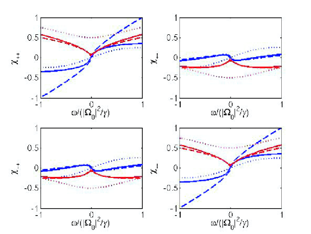
Figure 10: Self- and cross-susceptibilites (arbitrary units) $\chi_{\pm,\pm}(\omega)$ vs. frequency $\omega$ (in units of $|\Omega_{0}|^{2}/\gamma=(|\Omega_{+}|^{2}+|\Omega_{-}|^{2})/\gamma$), for $\Omega_{+}=\Omega_{-}$, $\Omega_{0}=0.1\gamma$. Real part (blue) and imaginary part (red), dotted line: Multiple spatial component approach truncated at $\mathcal{P}_{\pm 1}$, dashed line: Coupled Mode equations (analytic result), full line: Multiple spatial component approach truncated at $\mathcal{P}_{\pm(2n+1)}$ with $n=5$.

References

- [1] M.D Lukin, Rev. Mod. Phys. 75, 457-472 (2003).
- [2] M. Fleischhauer and M. D. Lukin, Phys. Rev. Lett. 84, 5094, (2000).
- [3] M. Fleischhauer and M. D. Lukin, Phys. Rev A 65, 022314 (2002).
- [4] B. Julsgaard et al, Nature 432, 482 (2004).
- [5] C. Liu et al, Nature 409, 490 (2001).
- [6] D. F. Phillips et al, Phys. Rev. Lett. 86, 783 (2001).
- [7] C. H. van der Wal et al., Science 301, 196 (2003).
- [8] A. Kuzmich et al., Nature 423, 731 (2003).
- [9] T. Chaneliere et al, Nature 438, 833 (2005).
- [10] M. D. Eisaman et al., Nature 438, 837 (2005).
- [11] M. D. Lukin et al., Phys. Rev. Lett. 87, 037901 (2001).
- [12] D. Tong et al, Phys. Rev. Lett. 93, 063001 (2004).
- [13] K. Singer et al, Phys. Rev. Lett. 93, 163001 (2004).
- [14] M. Bajcsy et al., Nature (London) 426, 638 (2003).
- [15] A. André et al, Phys. Rev. Lett. 94, 063902 (2005).
- [16] M. Fleischhauer, A. Imamoglu, and J. P. Marangos, Rev. Mod. Phys. 77, 633-673 (2005).
- [17] S. E. Harris, Phys. Rev. Lett. 70, 552 (1993).
- [18] M. Fleischhauer and A.S. Manka, Phys. Rev. A 54, 794 (1996).
- [19] S.E. Harris, Phys. Rev. Lett. 72, 52 (1994).
- [20] A.S. Zibrov et al. Phys. Rev. Lett. 88, 103601 (2002).
- [21] P. Arve, P. Jänes, and L. Thylen, Phys. Rev. A 69, 063809 (2004).
- [22] A.B. Matsko et al, Phys. Rev. A 64, 043809 (2001).
- [23] A. André, Nonclassical states of light and atomic ensembles: Generation and New Applications, Ph. D. Thesis, Harvard University, 2005.
- [24] C. W. Gardiner, Handbook of Stochastic Methods, (Spinger, Berlin, 1985)
- [25] S. A. Moiseev and B. S. Ham, Phys. Rev. A 71, 053802 (2005).
- [26] S. A. Moiseev and B. S. Ham, quant-ph/0512052 (2005).
- [27] A. Yariv and P. Yeh, Optical Waves in Crystals, (Wiley, New York, 1984).