Direct measurement of the quantum state of the electromagnetic field in a superconducting transmission line

Abstract

We propose an experimental procedure to directly measure the state of an electromagnetic field inside a resonator, corresponding to a superconducting transmission line, coupled to a Cooper-pair box (CPB). The measurement protocol is based on the use of a dispersive interaction between the field and the CPB, and the coupling to an external classical field that is tuned to resonance with either the field or the CPB. We present a numerical simulation that demonstrates the feasibility of this protocol, which is within reach of present technology

Superconducting electrical devices have been experimentally proven to be serious candidates for the realization of quantum information processing tasks makhlin:357 . Coherent control and near unit-visibility Rabi-oscillations wallraff:162 ; nakamura:246601 , coupling of two CPB-qubits pashkin:823 and the implementation of conditional gates yamamoto:941 are striking experiments that demonstrate the high level of control achieved on these systems. Furthermore, a scalable architecture for quantum computation has already been envisioned you:197902 .

On the other hand, recent demonstrations of Jaynes-Cummings-like dynamics between a CPB-qubit and the quantized mode of a superconducting transmission line resonator (which acts as a quasi-1D cavity) wallraff:162 ; blais:062320 have shown that many of the tools originally developed within the context of quantum optics can now be extended to solid state physics. Once coherent control and complete characterization of quantum states have been achieved at the qubit level, it is natural to attempt such levels of control for the electromagnetic field generated by the transmission line. For its characterization one could, in principle, make use of the well-known homodyne and heterodyne detection techniques. But, since the field we would like to characterize is inside a resonator and consists of a few photons, implementation of those techniques turns out to be a non-trivial task. Homodyne detection has been proposed for characterizing the state of the field leaking out from a tridimensional cavity in santos:033813 , and for a one-photon field leaking out of a 1-D cavity in solano . Nevertheless, it is very difficult to apply this procedure to high-finesse cavities containing weak fields, since one would have to distinguish a still weaker leaking field from the noise in the detector. Furthermore, unavoidable absorption losses may lead to poor reconstruction of the state of the intracavity field, as pointed out in khanbekyan:043807 .

To overcome these issues we propose here an experiment to directly measure the Wigner function wigner of the electromagnetic field inside a superconducting transmission line resonator coupled to a CPB-qubit, via the measurement of the latter’s populations. The Wigner function contains all the information about the state of the field, and is a useful tool for studying the decoherence-induced quantum-to-classical transition, as it provides us with a phase-space representation that can be compared to classical probability distributions toscano . For a single mode of the electromagnetic field, it is defined in terms of the respective density operator $\hat{\rho}$ as cahill :

$$W(\alpha)=(1/\pi){\rm Tr}[\hat{\rho}\hat{D}(\alpha)\hat{P}\hat{D}^{-1}(\alpha)].$$ (1)

Here, $\hat{D}(\alpha)=e^{\alpha\hat{a}^{\dagger}-\alpha^{*}\hat{a}}$ is the field displacement operator, which takes any coherent state $|\beta\rangle$ to $|\beta+\alpha\rangle$, up to a phase factor, and $\hat{P}=e^{-i\pi\hat{a}^{\dagger}\hat{a}}$ is the parity operator, which multiplies a Fock state $|n\rangle$ by a factor $(-1)^{n}$; $\hat{a}$ and $\hat{a}^{\dagger}$ are respectively the photon annihilation and creation operators of the mode. The displacement operator can be operationally implemented, in a cavity QED (cQED) setup raimond , by injecting a coherent field with complex amplitude $\alpha$ into the cavity. A protocol for the direct measurement of the Wigner function was first proposed in lutterbach:2547 and later experimentally carried out in nogues:054101 for the microwave field inside a 3-D high-quality-factor (Q) cavity. It involves injecting a microwave field (complex amplitude $\alpha$) into the cavity, so as to displace the field to be measured, and then sending an atom with two of its levels, $|e\rangle$ and $|g\rangle$, interacting dispersively with the displaced field. The atom is prepared in the state $(|e\rangle+|g\rangle)/\sqrt{2}$, and, after leaving the cavity, is submitted to a classical field, so that its state undergoes a $\pi/2$ rotation [$|e\rangle\rightarrow(|e\rangle+|g\rangle)/2$, $|g\rangle\rightarrow(-|e\rangle+|g\rangle)/2$]. Then the atomic population is measured. The difference between the probabilities of finding the atom in states $|e\rangle$ and $|g\rangle$ is proportional to the value of the Wigner function of the cavity field at the point $-\alpha$ in phase space.

It is not possible however to apply this protocol to the system here considered, since in this case the atom (CPB-qubit) is always inside the cavity and its interaction with the field cannot be turned off. Nevertheless, we show here that it is still possible to directly measure the Wigner function of the electromagnetic field in a superconducting transmission line, via the Copper-pair box qubit. Our method could also be applied to other systems involving the interaction of a qubit with a resonator geller .

The system under consideration consists of a mesoscopic superconducting island (see Fig. 1a) capacitively coupled to the quantized field mode of a transmission line of length $L$ (see Fig. 1b). Details of this system can be found in blais:062320 . The CPB Hamiltonian is given by makhlin:357 :

$$\hat{H}_{CPB}=4E_{C}(\hat{n}-n_{g})^{2}-E_{J}\cos\hat{\Theta}\,,$$ (2)

where $\hat{n}$ is the number operator corresponding to the Cooper-pair charges in excess on the island, and $\hat{\Theta}$ is the average phase drop along the junctions ($\hat{n}=-i\partial/\partial(\hat{\Theta})$). Each junction is characterized by a capacitance $C_{J}$ and a Josephson energy $E_{Jo}$. The effective Josephson coupling $E_{J}=2E_{Jo}\cos(\pi\Phi/\Phi_{o})$ can be changed through an applied static magnetic flux $\Phi$ ($\Phi_{o}=h/2e$ is the flux quantum and $e$ the electron charge). The charging energy is $E_{C}=e^{2}/2C_{\Sigma}$ ($C_{\Sigma}=C_{g}+2C_{J}$) and the gate charge is $n_{g}\equiv C_{g}V_{g}/2e$, which can be tuned by the dc part of the potential gate $V_{g}$. The coupling to the quantized field mode of the transmission line, of frequency $\omega$, is taken into account through the quantum part of the gate voltage, i.e. $V_{g}\equiv V_{g}^{\rm dc}+v$, where $v=\sqrt{\hbar\omega/Lc}\,(\hat{a}^{\dagger}+\hat{a})$ ($c$ is the transmission line capacitance per unit length), with $\hat{a}$ being the annihilation operator for the transmission-line mode. Finally, the Hamiltonian of the CPB-resonator system is obtained by adding, to Eq. (2), the Hamiltonian of the oscillator mode, i.e. $\hat{H}_{\rm os}=\hbar\omega\hat{a}^{\dagger}\hat{a}$. In the charge regime, i.e $\Delta_{\rm GAP}\gg E_{C}\gg 4\,E_{J}$ ($\Delta_{\rm GAP}$ is the superconductor gap) the CPB can be treated as an effective two-level system makhlin:357 of transition frequency $\omega_{0}=\sqrt{E_{J}^{2}+[4E_{C}(1-2\,n^{\rm dc}_{g})]^{2}}/\hbar$, with $n^{\rm dc}_{g}\equiv C_{g}V^{\rm dc}_{g}/2e$. Within this regime, when $n^{\rm dc}_{g}$ is around $1/2$ and in the rotating-wave approximation, the Hamiltonian of the composite system reduces to that of the Jaynes-Cummings (JC) model with coupling Rabi frequency $g=(eC_{g}/C_{\Sigma})\sqrt{\hbar\omega/Lc}$. In order to drive the composite system the transmission line is coupled capacitively ($C_{o}$) to an external classical microwave field, of frequency $\omega_{d}$ and slowly varying complex amplitude $\epsilon(t)=\epsilon_{R}(t)+i\epsilon_{I}(t)$, whose effect can be modeled through the driving Hamiltonian $\hat{H}_{d}=\hbar[\epsilon(t)\hat{a}^{\dagger}e^{-i\omega_{d}t}+H.c.]$. A second-order perturbative calculation, in the dispersive regime $|g\sqrt{\overline{n}+1}/\Delta|\ll 1$ ($\overline{n}$ is the mean photon number and $\Delta\equiv\omega_{0}-\omega$ is the detuning between the cavity and the CPB-qubit) yields, for the total system dynamics (including the driving), in a reference frame rotating with the driving field frequency, the effective Hamiltonian

$$\hat{H}^{int}_{eff}=\hbar(\omega-\omega_{d})\hat{a}^{\dagger}\hat{a}+\hbar\left[\epsilon(t)\hat{a}^{\dagger}+H.c.\right]+(\hbar/2)\vec{\Omega}\cdot\vec{\hat{\sigma}}\,,$$ (3)

where

$$\vec{\Omega} = \Big{[}(2g/\Delta)\epsilon_{R}(t),-(2g/\Delta)\epsilon_{I}(t),\omega_{0}-\omega_{d}$$ (4)

$$+ (g^{2}/\Delta)(2\hat{a}^{\dagger}\hat{a}+1)\Big{]}\,,$$

and $\vec{\hat{\sigma}}=(\hat{\sigma}_{x},\hat{\sigma}_{y},\hat{\sigma}_{z})$ are the Pauli matrices.

Hamiltonian (3) generates a displacement of the field but also induces a rotation on the qubit Bloch vector, the simultaneity of both operations coming from the impossibility of switching off the cavity-qubit interaction.

The measuring protocol consists of first encoding information contained in the initial field state, $\hat{\rho}$, into the CPB-qubit populations, which are then measured. The encoding process is divided into four evolution steps: 1) a coherent displacement of the field; 2) a $\pi/2$-pulse on the CPB-qubit; 3) a dispersive evolution without driving; and finally 4) another $\pi/2$-pulse on the CPB-qubit. The displacement of the field as well as the pulses on the qubit are driven by the external classical microwave field, whose complex amplitude $\epsilon(t)=\epsilon$ and frequency $\omega_{d}$ are the parameters under control.

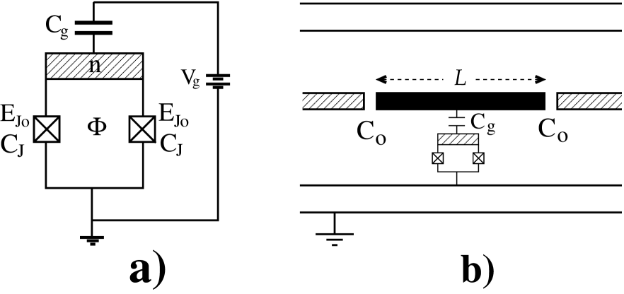
Figure 1: a) The Cooper-pair box: a superconducting island with $n$ Cooper pairs in excess (dashed area) with two Josephson Junctions (crossed boxes). b) Resonator-CPB-qubit composite system: the central superconducting waveguide (black) is coupled capacitively ($C_{0}$) to other two superconducting lines (dashed), through which the classical driving fields are pumped.

In the first step we set $\omega_{d}=\omega-g^{2}/\Delta$ and $\epsilon=\epsilon_{D}$, with $|\epsilon_{D}|\ll g+\Delta^{2}/2g$. This last condition implies, from (3) and (4), that we can neglect the components of the rotation axis $\vec{\Omega}$ perpendicular to the $z$-direction. So, if initially the qubit is in its ground state $|g\rangle$, it remains there, and the evolution operator in a reference frame rotating with frequency $\omega-g^{2}/\Delta$ is given by $\hat{U}_{\bf 1}(t_{D},0)=\hat{D}(\alpha)$, where $\alpha=-i\epsilon_{D}t_{D}$, and $t_{D}$ is the pulse duration.

In the second step we set the driving frequency $\omega_{d}=\omega_{0}$ and $\epsilon=|\epsilon_{\pi/2}|e^{i\phi_{1}}$, during a time $t_{\pi/2}=\pi\Delta/4g|\epsilon_{\pi/2}|$. Then, according to (4), each Fock component of the state suffers a $\pi/2$-rotation of the Bloch vector about an axis whose z-component, $(g^{2}/\Delta)(n+1/2)$, depends on the photon number $n$. This component can be neglected under the condition $|\epsilon_{\pi/2}|\gg g(\overline{n}+1/2)\Leftrightarrow\overline{n}\ll|\epsilon_{\pi/2}|/g-1/2$, where $\overline{n}$ is the mean number of photons in the state nota . In this case, the evolution operator is given by $\hat{U}_{\bf 2}(t_{D}+t_{\pi/2},t_{D})=e^{i\Delta\hat{a^{\dagger}}\hat{a}t_{\pi/2}}\hat{D}(\alpha_{\pi/2})\hat{R}_{\vec{n}}(\pi/2)$ in the representation rotating with frequency $\omega_{0}$ (which will be used from now on). This essentially consists of a displacement, $\hat{D}(\alpha_{\pi/2})$, of the field state by an amplitude $\alpha_{\pi/2}=-i\,e^{i\Delta t_{D}}\int^{t_{\pi/2}+t_{D}}_{t_{D}}\epsilon_{\pi/2}e^{-i\Delta t}dt$, and the rotation, $\hat{R}_{\vec{n}}(\pi/2)$, of the qubit state by an angle $\pi/2$ about an axis $\vec{\Omega}$ in the equatorial plane of the Bloch sphere.

In the third step we switch off the driving field, $\epsilon=0$, and let the system evolve freely during a time $t_{P}\equiv\pi\Delta/2g^{2}$ according to $\hat{U}_{\bf 3}(t_{D}+t_{\pi/2}+t_{P},t_{D}+t_{\pi/2})=e^{i\frac{\pi\Delta^{2}}{2g^{2}}\hat{a}^{\dagger}\hat{a}}e^{-i\frac{\pi}{2}(\hat{a}^{\dagger}\hat{a}+\frac{1}{2})\hat{\sigma}_{z}}$. Because the qubit is already in a superposition of the upper $|e\rangle$ and lower $|g\rangle$ states, this is the step where the field and the qubit get entangled, which is crucial for the transfer of information from the field to the qubit. The fourth and last step in the encoding process is another $\pi/2$-pulse on the qubit, with $\epsilon\equiv|\epsilon_{\pi/2}|e^{i\phi_{2}}$, corresponding to an evolution operator $\hat{U}_{\bf 4}$ analogous to $\hat{U}_{2}$.

Collecting all the steps of the encoding process we get the total evolution $\hat{U}_{T}=\hat{U}_{4}\hat{U}_{3}\hat{U}_{2}\hat{U}\hat{U}_{1}$, where $\hat{U}=e^{i(\Delta+g^{2}/\Delta)\big{(}\hat{a}^{\dagger}\hat{a}+\hat{\sigma}_{z}/2\big{)}t_{D}}$ switches from a frame rotating with frequency $\omega-g^{2}/\Delta$ to one rotating with frequency $\omega_{0}$. Thus, $\langle\hat{\sigma}_{z}\rangle\equiv P_{e}-P_{g}\equiv{\rm Tr}[\hat{\sigma}_{z}\hat{U}_{T}|g\rangle\langle g|\hat{\rho}\,\hat{U}^{\dagger}_{T}]$ is straightforwardly calculated, yielding

$$P_{e}-P_{g}=Tr\Big{[}\sin(\phi_{1}-\phi_{2})\hat{\rho}\hat{D}(\beta)^{\dagger}e^{-i\pi\hat{a}^{\dagger}\hat{a}}\hat{D}(\beta)\Big{]}\,,$$ (5)

where $\beta\equiv\alpha+(2|\epsilon_{\pi/2}|/\Delta)\sin(t_{\pi/2}\Delta/2)e^{-i\phi}$, with $\alpha=-i\epsilon_{D}t_{D}$ and $\phi=(t_{D}+t_{\pi/2}/2)\Delta+g^{2}t_{D}/\Delta+\pi/2-\phi_{1}$. When $\phi_{1}-\phi_{2}=\pi/2$ we see from Eq. (1) that $\langle\hat{\sigma}_{z}\rangle/\pi$ yields the value of the initial-field Wigner function at the point $-\beta$. If the first $\pi/2$-pulse is chosen so that $t_{\pi/2}\Delta/2=m\pi$, $m$ integer, then $\beta=\alpha$. By repeating the experiment for different $t_{D}$ s one can scan the whole phase space and thus fully reconstruct the quantum state.

$\Delta$	$g$	$|\epsilon_{D}|$	$|\epsilon_{\pi/2}|$	$\kappa^{-1}$	$\gamma^{-1}$
$0.1$	$5\times 10^{-3}$	$0.025$	$0.025$	$160$ ns	$2\mu$s
$0.3$	$5\times 10^{-3}$	$0.025$	$0.281$	$1000$ ns	$2\mu$s

Table 1: Experimental parameters. $\Delta$, $g$, $\epsilon_{D}$, and $\epsilon_{\pi/2}$ are expressed in units of the transmission line frequency. The first set of parameters is reported in blais:062320 ; the second is the proposed one. $\kappa^{-1}$ is the cavity lifetime and $\gamma^{-1}$ is the atom lifetime.

Table 1 displays a comparison between the parameters reported in blais:062320 and the optimal parameters that we propose. The performance of the protocol for these two sets of parameters were tested by a numerical simulation, where each step of the protocol was carried out evolving the system with the exact JC-model plus the driving Hamiltonian. The Wigner function of the field state was obtained using Eq. (5) where the probabilities $P_{e}$ and $P_{g}$ were calculated for the final entangled state of the system (see Fig. 2). With the first set of parameters, the whole measurement protocol takes approximately $100$ ns, which is less than the cavity lifetime $\kappa^{-1}$ and much smaller than the atom lifetime $\gamma^{-1}$. Moreover, the condition $|\epsilon_{D}|\ll g+\Delta^{2}/2g\approx\Delta^{2}/2g=\omega$, used in the first step of the protocol, is well satisfied. On the other hand, we see that the condition for the $\pi/2$ rotation is not comfortably met, since it is not true that $\overline{n}\ll|\epsilon_{\pi/2}|/g-1/2=4.5$ for the states of interest. In fact, because the mean photon number increases after the displacement of the field in the first step, i.e. $\overline{n}\rightarrow\overline{n}+2\Re e(\alpha^{*}\langle\hat{a}\rangle)+|\alpha|^{2}$, the conditions for the $\pi/2$ rotation and the dispersive regime approximation are violated for greater values of $|\alpha|$ (see the numerical points on the tails of the graphs on the left in Fig.(2)). During the $\pi/2$ rotation of the CPB-qubit the field is also displaced to $\beta=\alpha+(2|\epsilon_{\pi/2}|/\Delta)\sin(t\Delta/2)e^{-i\phi}$, so the displacement $|\beta-\alpha|$ attains its maximum value at the middle of the rotation, violating the dispersive-regime approximation for the first set of parameters. These considerations imply that the accuracy of the method is worse for the tails of the Wigner functions, since probing them requires larger displacements of the cavity field. The poor accuracy in Fig. 2(c1) is due to the contribution of high-$n$ Fock states. Finally, one should consider that with $\kappa^{-1}=160$ ns decoherence effects may become appreciable at $100$ ns (duration of the measurement protocol in this case) for fields with average photon number larger than one. Thus, a higher-Q cavity should be required.

Figure 2: Wigner function $W(\alpha)$ on the real axis $\alpha=x$ for different states of the cavity field: (a1) and (a2) Vacuum state; (b1) and (b2) Fock state with $n=1$; (c1) and (c2) Schrödinger-cat state $\propto(|\alpha_{0}\rangle-|-\alpha_{0}\rangle)$, with $\alpha_{0}=2$. The full line is the theoretical value and the crosses stand for the values obtained by a numerical simulation of the measurement protocol (see text for details). The numerical simulations on the left-hand (right-hand) side were performed with the first (second) row of parameters in Table 1. The transmission line frequency is taken as $\omega=2\pi\times 10\,GHz$.

With the detuning proposed in the second set of parameters the total duration of the protocol would be about $300$ ns, for a cavity lifetime $\kappa^{-1}\sim 1000$ ns. The difference of one order of magnitude between the values for the damping times in the two sets of parameters in Table I is easily overcome with present technology. Better lifetimes could be achieved, for example, by decreasing the value of the capacitances $C_{0}$. On the other hand, $|\epsilon_{\pi/2}|$ increases with the power of the external radio-frequency source. The improvement in the reconstruction of the Wigner function for this second set of parameters is displayed in the graphs on the right-hand side of Fig. 2, for the vacuum state, the Fock state with $n=1$, and a Schrödinger- cat state. The main impact of using the new parameters is a great reduction of the errors in the tails of the Wigner functions. Decoherence, not taken into account in our simulations, would further limit the maximum number of photons in the states characterized. Temperature effects are negligible for typical experimental values ($T=100$ mK in wallraff:162 ). Indeed, for $T=100$ mK, and given that for our parameters we have $\hbar\omega/k\approx 480$ mK, the thermal occupation number is $\bar{n}<0.008$. The reconstruction of states with more photons would demand higher Q’s, but the protocol would remain the same. We note that the experiment could be used to continuously monitor the loss of coherence of the field.

As for the measurement of the qubit population, a dispersive quantum non-demolition scheme was carried out in wallraff:162 . However, for the higher Q value considered here, this technique would take a time of the order of the qubit lifetime. The direct measurement of the qubit population could be accomplished in this case by coupling to the qubit a single electron transistor (SET) device, which is able to detect charge differences of the order of $e$, as described, for example, in astafiev:180507 . The influence of the SET on the qubit dynamics can be minimized by turning the device on only at the moment of measurement, as discussed in astafiev:180507 . The presence of an extra superconducting lead connecting the SET to the qubit should not increase significantly the decoherent effects on the cavity field already introduced by the presence of the Cooper-pair box.

Experimental testing of this protocol would require the preparation of simple field states. Coherent states are prepared by displacing the initial state $|g,0\rangle$, which is accomplished by setting the driving parameters $\omega_{d}=\omega-g^{2}/\Delta$ and $\epsilon=\epsilon_{D}$, as in the first step of our protocol. This will take a time $t_{D}=|\alpha|/|\epsilon_{D}|$ to be carried out, where $\alpha$ is the amplitude of the coherent state. The generation of a Schrödinger cat-like state, i.e. $(|\alpha_{0}\rangle\pm e^{i\varphi}|-{\alpha_{0}}\rangle)/N$, where $N$ is a normalization factor, is contained implicitly in the protocol described in this paper, since after the whole evolution stage, and before the qubit population is measured, the final entangled state of the system is of the type $(1/\sqrt{2})(|{\alpha_{0}}\rangle+\,e^{i\varphi}\,|-{\alpha_{0}}\rangle)\otimes|e\rangle$ $+(1/\sqrt{2})(|{\alpha_{0}}\rangle-\,e^{i\varphi}\,|-{\alpha_{0}}\rangle)\otimes|g\rangle$. Measuring the qubit population would project this state onto a coherent superposition of two coherent states. The time required to generate this state is the same as for our protocol.

Another example of interest is the one-photon Fock state: beginning with the system in the state $|g,0\rangle$ one applies a $\pi$-pulse on the qubit, setting $\omega_{d}=\omega_{0}$ and $\epsilon=\epsilon_{\pi}$ during a time $t_{\pi}=\pi\Delta/2g|\epsilon_{\pi}|$. Choosing $t_{\pi}\Delta/2=m\pi$, with $m$ integer, the state $|e,0\rangle$ is prepared. Then, we tune the qubit frequency $\omega_{0}$ into resonance with the cavity mode (by changing the magnetic flux $\Phi$) and let the system complete a Rabi oscillation ($t_{Ra}=\pi/2g$), so the resulting state is $|g,1\rangle$. Next we change the magnetic flux again to take the system back to the dispersive regime. This method would require rapid switching of the flux (less than 1 ns), a challenge for present experiments. Alternatively, time-dependent magnetic fluxes could be used to tune the qubits into and out of resonance with the cavity field, as recently suggested in nori2 . For the second set of parameters in Table 1 and $|\epsilon_{\pi}|=0.3\,\omega$ ($m=15$) the total time for this process would then be $t_{Ra}+t_{\pi}\sim 10$ ns.

In conclusion, we propose here an experiment to completely characterize the electromagnetic field of a quasi 1-D superconducting transmission line resonator, which is always interacting with a CPB-qubit, by directly measuring its Wigner function. This is carried out by measuring the CPB-qubit population after the application of a series of driving pulses, induced by an external microwave field coupled to the resonator. Our numerical simulations, for realistic parameters, show that this method is within reach of present experimental setups.

We thank F. Schackert and C. H. Lewenkopf for useful discussions and CAPES, CNPq, FAPERJ, and the Millennium Institute for Quantum Information for support.

References

- (1) Y. Makhlin, G. Schon, and A. Shnirman, Rev. Mod. Phys. 73, 357 (2001).
- (2) A. Wallraff et al., Nature 431, 162 (2004).
- (3) Y. Nakamura, Y. A. Pashkin, and J. S. Tsai, Phys. Rev. Lett. 87, 246601 (2001); Y. Yu et al., Science 296, 889 (2002); D. Vion et al., Science 296, 886 (2002); A. Wallraff et al., Phys. Rev. Lett. 95, 060501 (2005).
- (4) Y. A. Pashkin et al., Nature 421, 823 (2003).
- (5) T. Yamamoto et al., Nature 425, 941 (2003).
- (6) J. Q. You, J. S. Tsai, and F. Nori, Phys. Rev. Lett. 89, 197902 (2002).
- (7) A. Blais et al., Phys. Rev. A 69, 062320 (2004).
- (8) M. F. Santos et al., Phys. Rev. A 63, 033813 (2001).
- (9) M. Mariantoni et al., cond-mat/0509737 (2005).
- (10) M. Khanbekyan et al., Phys. Rev. A 69, 043807 (2004).
- (11) E. Wigner, Phys. Rev. 40, 749 (1932).
- (12) F. Toscano, R. L. de Matos Filho, and L. Davidovich, Phys. Rev. A 71, 010101(R) (2005).
- (13) K. E. Cahill and R. J. Glauber, Phys. Rev. 177, 1857 (1969); 177, 1882 (1969).
- (14) J. M. Raimond, M. Brune, and S. Haroche, Rev. Mod. Phys. 73, 565 (2001).
- (15) L. G. Lutterbach and L. Davidovich, Phys. Rev. Lett. 78, 2547 (1997).
- (16) G. Nogues et al., Phys. Rev. A 62, 054101 (2000).
- (17) A. S. Sorensen et al., Phys. Rev. Lett. 92, 063601 (2004); L. Tian et al., Phys. Rev. Lett. 92, 247902 (2004); A. N. Cleland and M. R. Geller, Phys. Rev. Lett. 93, 070501 (2004).
- (18) Strictly speaking, we should impose this condition to every photon number present in the state; or, alternatively, ask that the distribution in photon number be very localized around .
- (19) O. Astafiev et al., Phys. Rev. B 69, 180507(R) (2004).
- (20) L. Davidovich et al., Phys. Rev. A 53, 1295 (1996).
- (21) Yu-xi Liu et al., cond-mat/0507496.