A probabilistic operator symbol framework for quantum information

Abstract

Hilbert space operators may be mapped onto a space of ordinary functions (operator symbols) equipped with an associative (but noncommutative) star-product. A unified framework for such maps is reviewed. Because of its clear probabilistic interpretation, a particular class of operator symbols (tomograms) is proposed as a framework for quantum information problems. Qudit states are identified with maps of the unitary group into the simplex. The image of the unitary group on the simplex provides a geometrical characterization of the nature of the quantum states. Generalized measurements, typical quantum channels, entropies and entropy inequalities are discussed in this setting.

1 Introduction

Algebras of Hilbert space operators may be mapped onto algebras of ordinary functions on linear spaces, with an associative but non-commutative star product (see, e.g. [1, 2]). The images of the Hilbert space operators are called operator symbols. Weyl maps [3, 4], $s$-ordered operator symbols [5], their partial cases [6, 7, 8, 9] and tomograms [10, 11, 12] are examples of this correspondence between Hilbert space operator algebras and function algebras [13, 14]. In the case of tomograms, the operator symbols of the density operators of quantum mechanics are families of ordinary probability distributions [15, 16, 13, 17].

A unified framework for operator symbols is presented in Sect. 2 and their main properties are reviewed. Many of the results in Sects. 2 and 3 are scattered in previous publications and are collected here to make the paper reasonably self-contained.

Finite dimensional systems (spin tomograms) are studied in Sect. 3. These operator symbols are then proposed as a framework for quantum information problems. Qudit states are identified with maps of the unitary group into the simplex. The image of the unitary group on the simplex provides a geometrical characterization of the nature of the quantum states. In the remaining sections, generalized measurements, typical quantum channels, entropies and entropy inequalities are discussed in this setting.

2 Operator symbols for quantum mechanical observables

In quantum mechanics, observables are selfadjoint operators acting on the Hilbert space of states $H$. We map operators onto functions in a vector space $X$ in the following way:

Given the Hilbert space $H$ and a trace-class operator $\hat{A}$ acting on this space, let $\hat{U}(\mathbf{x})$ be a family of operators on $H$, labelled by vectors $\mathbf{x\in X}$. We construct the $c$-number function $\left\{f_{\hat{A}}(\mathbf{x}):X\rightarrow\mathbb{C}\right\}$ (and call it the symbol of the operator $\hat{A}$) by

$$f_{\hat{A}}(\mathbf{x})=\mbox{Tr}\left[\hat{A}\hat{U}(\mathbf{x})\right].$$ (1)

Let us suppose that relation (1) has an inverse, i.e., there is a set of operators $\hat{D}(\mathbf{x})$ acting on the Hilbert space such that

$$\hat{A}=\int_{X}f_{\hat{A}}(\mathbf{x})\hat{D}(\mathbf{x})~{}d\mathbf{x},\qquad\mbox{Tr}\,\hat{A}=\int_{X}f_{\hat{A}}(\mathbf{x})\,\mbox{Tr}\,\hat{D}(\mathbf{x})~{}d\mathbf{x}.$$ (2)

Equations (1) and (2) define an invertible map from the operator $\hat{A}$ onto the function $f_{\hat{A}}(\mathbf{x})$. Multiplying both sides of Eq.(2) by the operator $\hat{U}(\mathbf{x}^{\prime})$ and taking the trace, one obtains a consistency condition for the operators $\hat{U}(\mathbf{x}^{\prime})$ and $\hat{D}(\mathbf{x})$

$$\mbox{Tr}\left[\hat{D}(\mathbf{x})\hat{U}(\mathbf{x}^{\prime})\right]=\delta\left(\mathbf{x-x}^{\prime}\right).$$

For two functions $f_{\hat{A}}(\mathbf{x})$ and $f_{\hat{B}}(\mathbf{x})$, corresponding to two operators $\hat{A}$ and $\hat{B}$, a star-product is defined by

$$f_{\hat{A}\hat{B}}(\mathbf{x})=f_{\hat{A}}(\mathbf{x})*f_{\hat{B}}(\mathbf{x}):=\mbox{Tr}\left[\hat{A}\hat{B}\hat{U}(\mathbf{x})\right].$$ (3)

Since the standard product of operators on a Hilbert space is associative, Eq. (3) also defines an associative product for the functions $f_{\hat{A}}(\mathbf{x})$, i.e.,

$$f_{\hat{A}}(\mathbf{x})*\Big{(}f_{\hat{B}}(\mathbf{x})*f_{\hat{C}}(\mathbf{x})\Big{)}=\Big{(}f_{\hat{A}}(\mathbf{x})*f_{\hat{B}}(\mathbf{x})\Big{)}*f_{\hat{C}}(\mathbf{x}).$$ (4)

Let us suppose that there is another map, analogous to the one in (1) and (2), defined by the operator families $\hat{U}_{1}(\mathbf{y})$ and $\hat{D}_{1}(\mathbf{y})$. Then one has

$$\phi_{\hat{A}}(\mathbf{y})=\mbox{Tr}\left[\hat{A}\hat{U}_{1}(\mathbf{y})\right]$$ (5)

and the inverse relation

$$\hat{A}=\int\phi_{A}(\mathbf{y})\hat{D}_{1}(\mathbf{y})~{}d\mathbf{y}.$$ (6)

The function $f_{\hat{A}}(\mathbf{x})$ will be related to the function $\phi_{\hat{A}}(\mathbf{y})$ by

$$\phi_{\hat{A}}(\mathbf{y})=\int f_{\hat{A}}(\mathbf{x})\,\mbox{Tr}\left[\hat{D}(\mathbf{x})\hat{U}_{1}(\mathbf{y})\right]\,d\mathbf{x}$$ (7)

with the inverse relation

$$f_{\hat{A}}(\mathbf{x})=\int\phi_{\hat{A}}(\mathbf{y})\,\mbox{Tr}\left[\hat{D}_{1}(\mathbf{y})\hat{U}(\mathbf{x})\right]\,d\mathbf{y}.$$ (8)

The functions $f_{\hat{A}}(\mathbf{x})$ and $\phi_{\hat{A}}(\mathbf{y})$, corresponding to different maps, are connected by the invertible integral transform given by Eqs.(7) and (8) with the intertwining kernels

$$K_{1}(\mathbf{x},\mathbf{y})=\mbox{Tr}\,\Big{[}\hat{D}(\mathbf{x})\hat{U}_{1}(\mathbf{y})\Big{]}$$ (9)

and

$$K_{2}(\mathbf{x},\mathbf{y})=\mbox{Tr}\,\Big{[}\hat{D}_{1}(\mathbf{y})\hat{U}(\mathbf{x})\Big{]}.$$ (10)

Using formulae (1) and (2), one writes a composition rule for two symbols $f_{\hat{A}}(\mathbf{x})$ and $f_{\hat{B}}(\mathbf{x})$determining their star-product

$$f_{\hat{A}}(\mathbf{x})*f_{\hat{B}}(\mathbf{x})=\int f_{\hat{A}}(\mathbf{x}^{\prime\prime})f_{\hat{B}}(\mathbf{x}^{\prime})K(\mathbf{x}^{\prime\prime},\mathbf{x}^{\prime},\mathbf{x})\,d\mathbf{x}^{\prime}\,d\mathbf{x}^{\prime\prime}.$$ (11)

The kernel in (11) is determined by the trace of the product of the operators used to construct the map

$$K(\mathbf{x}^{\prime\prime},\mathbf{x}^{\prime},\mathbf{x})=\mbox{Tr}\left[\hat{D}(\mathbf{x}^{\prime\prime})\hat{D}(\mathbf{x}^{\prime})\hat{U}(\mathbf{x})\right].$$ (12)

Equation (12) can be extended to the case of the star-product of $N$ symbols of operators $\hat{A}_{1},\hat{A}_{2},\ldots,\hat{A}_{N}$

$$f_{\hat{A}_{1}}(\mathbf{x})*f_{\hat{A}_{2}}(\mathbf{x})*\cdots*f_{\hat{A}_{N}}(\mathbf{x}) = \int f_{\hat{A}_{1}}(\mathbf{x}_{1})f_{\hat{A}_{2}}(\mathbf{x}_{2})\cdots f_{\hat{A}_{N}}(\mathbf{x}_{N})$$

$$\times K\left(\mathbf{x}_{1},\mathbf{x}_{2},\ldots,\mathbf{x}_{N},\mathbf{x}\right)\,d\mathbf{x}_{1}\,d\mathbf{x}_{2}\cdots\,d\mathbf{x}_{N}$$

with kernel

$$K\left(\mathbf{x}_{1},\mathbf{x}_{2},\ldots,\mathbf{x}_{N},\mathbf{x}\right)=\mbox{Tr}\left[\hat{D}(\mathbf{x}_{1})\hat{D}(\mathbf{x}_{2})\cdots\hat{D}(\mathbf{x}_{N})\hat{U}(\mathbf{x})\right].$$ (14)

The trace of an operator $\hat{A}^{N}$ is determined by

$$\mbox{Tr}\,\hat{A}^{N}=\int f_{\hat{A}}(\mathbf{x}_{1})f_{\hat{A}}(\mathbf{x}_{2})\cdots f_{\hat{A}}(\mathbf{x}_{N})$$

$$\times\mbox{Tr}\left[\hat{D}(\mathbf{x}_{1})\hat{D}(\mathbf{x}_{2})\cdots\hat{D}(\mathbf{x}_{N})\right]\,d\mathbf{x}_{1}\,d\mathbf{x}_{2}\cdots\,d\mathbf{x}_{N}.$$ (15)

Consider now a linear superoperator $L$ acting in linear space of operators. The map of operators $\hat{A}\rightarrow L\hat{A}$ induces a corresponding map of their symbols

$$f_{\hat{A}}(\mathbf{x})\rightarrow\hat{L}f_{\hat{A}}(\mathbf{x})=f_{L\hat{A}}(\mathbf{x}).$$ (16)

The integral form of this map

$$\hat{L}f_{\hat{A}}(\mathbf{x})=\int\Pi_{L}(\mathbf{x},\mathbf{x}^{\prime})f_{\hat{A}}(\mathbf{x}^{\prime})\,d\mathbf{x}^{\prime}$$ (17)

is determined by the kernel

$$\Pi_{L}(\mathbf{x},\mathbf{x}^{\prime})=\mbox{Tr}\left[\hat{U}(\mathbf{x})\Big{(}L\hat{D}(\mathbf{x}^{\prime})\Big{)}\right].$$ (18)

2.1 The Weyl operator symbols

As operator family $\hat{U}(\mathbf{x})$, we take the Fourier transform of the displacement operator $d(\xi)$

$$\hat{U}(\mathbf{x})=\int\exp\left(\frac{x_{1}+ix_{2}}{\sqrt{2}}\mbox{\boldmath$\xi$}^{*}-\frac{x_{1}-ix_{2}}{\sqrt{2}}\mbox{\boldmath$\xi$}\right)d(\mbox{\boldmath$\xi$})\pi^{-1}~{}d^{2}\mbox{\boldmath$\xi$},$$ (19)

where $\xi$ is a complex number, $\mbox{\boldmath$\xi$}=\xi_{1}+i\xi_{2}$, and the vector $\mathbf{x}=(x_{1},x_{2})$ may be interpreted as $\mathbf{x}=(q,p)$, with $q$ and $p$ being the position and momentum. One sees that $\mbox{Tr}\,\hat{U}(\mathbf{x})=1$. The displacement operator (creating coherent states from the vacuum) may be expressed through creation and annihilation operators in the form

$$d(\mbox{\boldmath$\xi$})=\exp(\mbox{\boldmath$\xi$}\hat{a}^{\dagger}-\mbox{\boldmath$\xi$}^{*}\hat{a}),$$ (20)

$$\hat{a}=\frac{\hat{q}+i\hat{p}}{\sqrt{2}},\qquad\hat{a}^{\dagger}=\frac{\hat{q}-i\hat{p}}{\sqrt{2}}.$$ (21)

The operator $\hat{a}$ and its Hermitian conjugate $\hat{a}^{\dagger}$ satisfy the boson commutation relation $[\hat{a},\hat{a}^{\dagger}]=\hat{\mathbf{1}}.$

The Weyl symbol for an operator $\hat{A}$ reads

$$W_{\hat{A}}(\mathbf{x})=\mbox{Tr}\left[\hat{A}\hat{U}(\mathbf{x})\right],$$ (22)

$\hat{U}(\mathbf{x})$ being given by Eq.(19). The Weyl symbols of the identity operator $\hat{\mathbf{1}}$, the position operator $\hat{q}$ and the momentum operator $\hat{p}$ are

$$W_{\hat{\mathbf{1}}}(q,p)=1\qquad W_{\hat{q}}(q,p)=q\qquad W_{\hat{p}}(q,p)=p.$$ (23)

The inverse transform, which expresses the operator $\hat{A}$ through its Weyl symbol, is

$$\hat{A}=\int W_{\hat{A}}(\mathbf{x})\hat{U}(\mathbf{x})\,\frac{d\mathbf{x}}{2\pi}\,.$$ (24)

That is, the operator $\hat{D}(\mathbf{x})$ in formula (2) is related to $\hat{U}(\mathbf{x})$ by

$$\hat{D}(\mathbf{x})=\frac{\hat{U}(\mathbf{x})}{2\pi}\,.$$ (25)

The star-product of the Weyl symbols of two operators $\hat{A}_{1}$ and $\hat{A}_{2}$ , expressed through Weyl symbols by

$$\hat{A}_{1}=\int W_{\hat{A}_{1}}(\mathbf{x}^{\prime})\hat{U}(\mathbf{x}^{\prime})\,\frac{d\mathbf{x}^{\prime}}{2\pi},\qquad\hat{A}_{2}=\int W_{\hat{A}_{2}}(\mathbf{x}^{\prime\prime})\hat{U}(\mathbf{x}^{\prime\prime})\,\frac{d\mathbf{x}^{\prime\prime}}{2\pi},$$ (26)

with vectors $\mathbf{x}^{\prime}=(x_{1}^{\prime},x_{2}^{\prime})$ and $\mathbf{x}^{\prime\prime}=(x_{1}^{\prime\prime},x_{2}^{\prime\prime})$, is the operator $\hat{A}$ with Weyl symbol

$$W_{\hat{A}}(\mathbf{x})=W_{\hat{A}_{1}}(\mathbf{x})*W_{\hat{A}_{2}}(\mathbf{x})=\int\frac{d\mathbf{x}^{\prime}\,d\mathbf{x}^{\prime\prime}}{\pi^{2}}\,W_{\hat{A}_{1}}(\mathbf{x}^{\prime})W_{\hat{A}_{2}}(\mathbf{x}^{\prime\prime})$$

$$\times\exp\Big{\{}2i\Big{[}(x_{2}^{\prime}-x_{2})(x_{1}-x_{1}^{\prime\prime})+(x_{1}^{\prime}-x_{1})(x_{2}^{\prime\prime}-x_{2})\Big{]}\Big{\}}.$$ (27)

2.2 The $s$-ordered operator symbols

The $s$-ordered symbol [5] $W_{\hat{A}}(\mathbf{x},s)$ of the operator $\hat{A}$ is

$$W_{\hat{A}}(\mathbf{x},s)=\mbox{Tr}\left[\hat{A}\hat{U}(\mathbf{x},s)\right],$$ (28)

with a real parameter $s$, real vector $\mathbf{x}=(x_{1},x_{2})$ and operator $\hat{U}(\mathbf{x},s)$

$$\hat{U}(\mathbf{x},s)=\frac{2}{1-s}\,d(\alpha_{\mathbf{x}})\,q^{\hat{a}^{\dagger}\hat{a}}(s)\,d(-\alpha_{\mathbf{x}}),$$ (29)

the displacement operator being

$$d(\alpha_{\mathbf{x}})=\exp\left(\alpha_{\mathbf{x}}\hat{a}^{\dagger}-\alpha_{\mathbf{x}}^{*}\hat{a}\right).$$ (30)

Also

$$\alpha_{\mathbf{x}}=x_{1}+ix_{2},\qquad\alpha_{\mathbf{x}}^{*}=x_{1}-ix_{2},\qquad x_{1}=\frac{q}{\sqrt{2}},\qquad x_{2}=\frac{p}{\sqrt{2}}$$ (31)

and

$$q(s)=\frac{s+1}{s-1}\,.$$ (32)

The coefficient in Eq. (29) leads to $\mbox{Tr}\left[\hat{U}(\mathbf{x},s)\right]=1$, meaning that the symbol of the identity operator equals $1$.

The operator $\hat{A}$ is obtained from

$$\hat{A}=\frac{1}{\pi}\,\frac{1+s}{1-s}\,\int W_{\hat{A}}(\mathbf{x},s)\hat{U}(\mathbf{x},-s)\,d(\mathbf{x}).$$ (33)

This means that, for $s$-ordered symbols, the operator $\hat{D}(\mathbf{x})$ in the general formula (2) takes the form

$$\hat{D}(\mathbf{x})=\frac{1}{\pi}\,\frac{1+s}{1-s}\,\hat{U}(\mathbf{x},-s).$$ (34)

If $\hat{A}$ is a density operator $\hat{\rho}$ [18, 19, 20], for the values of the parameters $s=0,1,-1$, the corresponding symbols are respectively the Wigner, Glauber–Sudarshan and Husimi quasidistributions.

For the explicit form of the kernel for the product of $N$ operator symbols we refer to [13].

2.3 The tomographic operator symbols

Density operators may be mapped onto probability distribution functions (tomograms) of one random variable $X$ and two real parameters $\mu$ and $\nu$. This map has been used to provide a formulation of quantum mechanics, in which quantum states are described by a parametrized family of probability distributions [15, 16], alternative to the description of the states by wave functions or density operators. The tomographic map has been used to reconstruct the quantum state, to obtain the Wigner function by measuring the state tomogram, to define quantum characteristic exponents [21] and for the simulation of nonstationary quantum systems [22].

Here we discuss the tomographic map as an example of the general operator symbol framework. The operator $\hat{A}$ is mapped onto the function $f_{\hat{A}}(\mathbf{x})$, where $\mathbf{x}\equiv(X,\mu,\nu)$, which we denote as $w_{\hat{A}}(X,\mu,\nu)$ depending on the coordinate $X$ and the reference frame parameters $\mu$ and $\nu$

$$w_{\hat{A}}(X,\mu,\nu)=\mbox{Tr}\left[\hat{A}\hat{U}(\mathbf{x})\right].$$ (35)

The function $w_{\hat{A}}(X,\mu,\nu)$ is the symbol of the operator $\hat{A}$. The operator $\hat{U}(x)$ is

$$\hat{U}(\mathbf{x}) \equiv \hat{U}(X,\mu,\nu)=\exp\left(\frac{i\lambda}{2}\left(\hat{q}\hat{p}+\hat{p}\hat{q}\right)\right)\exp\left(\frac{i\theta}{2}\left(\hat{q}^{2}+\hat{p}^{2}\right)\right)\mid X\rangle\langle X\mid$$

$$\qquad~{}\times\exp\left(-\frac{i\theta}{2}\left(\hat{q}^{2}+\hat{p}^{2}\right)\right)\exp\left(-\frac{i\lambda}{2}\left(\hat{q}\hat{p}+\hat{p}\hat{q}\right)\right)$$

$$= \hat{U}_{\mu\nu}\mid X\rangle\langle X\mid\hat{U}_{\mu\nu}^{\dagger},$$ (36)

where $\hat{q}$ and $\hat{p}$ are position and momentum operators and the angle $\theta$ and parameter $\lambda$ are related to the reference frame parameters by

$$\mu=e^{\lambda}\cos\theta\qquad\nu=e^{-\lambda}\sin\theta.$$

Moreover,

$$\hat{X}\mid X\rangle=X\mid X\rangle$$ (37)

and $\mid X\rangle\langle X\mid$ is a projection density. One has the canonical transform of quadratures

$$\hat{X}=\hat{U}_{\mu\nu}\,\hat{q}\,\hat{U}_{\mu\nu}^{\dagger}=\mu\hat{q}+\nu\hat{p},$$

$$\hat{P}=\hat{U}_{\mu\nu}\,\hat{p}\,\hat{U}_{\mu\nu}^{\dagger}=\frac{1+\sqrt{1-4\mu^{2}\nu^{2}}}{2\mu}\,\hat{p}-\frac{1-\sqrt{1-4\mu^{2}\nu^{2}}}{2\nu}\,\hat{q}.$$

Using the approach of [23] one obtains the relation

$$\hat{U}(X,\mu,\nu)=\delta(X-\mu\hat{q}-\nu\hat{p}).$$

In the case we are considering, the inverse transform determining the operator in terms of the tomogram symbol will be of the form

$$\hat{A}=\int w_{\hat{A}}(X,\mu,\nu)\hat{D}(X,\mu,\nu)\,dX\,d\mu\,d\nu,$$ (38)

where [24, 10]

$$\hat{D}(\mathbf{x})\equiv\hat{D}(X,\mu,\nu)=\frac{1}{2\pi}\exp\left(iX-i\nu\hat{p}-i\mu\hat{q}\right),$$ (39)

i.e.,

$$\hat{D}(X,\mu,\nu)=\frac{1}{2\pi}\exp(iX)d\Big{(}\mbox{\boldmath$\xi$}(\mu,\nu)\Big{)}.$$ (40)

The unitary displacement operator in (40) now reads

$$d\Big{(}\mbox{\boldmath$\xi$}(\mu,\nu)\Big{)}=\exp\Big{(}\mbox{\boldmath$\xi$}(\mu,\nu)\hat{a}^{+}-{\mbox{\boldmath$\xi$}}^{*}(\mu,\nu)\hat{a}\Big{)},$$

where $\mbox{\boldmath$\xi$}(\mu,\nu)=\xi_{1}+i\xi_{2}$ with $\xi_{1}=\mbox{Re}\,(\mbox{\boldmath$\xi$})={\nu}/{\sqrt{2}}$ and $\xi_{2}=\mbox{Im}\,(\mbox{\boldmath$\xi$})=-{\mu}/{\sqrt{2}}$.

The trace of the above operator provides the kernel determining the trace of an arbitrary operator in the tomographic representation

$$\mbox{Tr}\,\hat{D}(\mathbf{x})=e^{iX}\delta(\mu)\delta(\nu).$$

The operators $a^{\dagger}$ and $a$ are creation and annihilation operators. The function $w_{\hat{A}}(X,\mu,\nu)$ satisfies the relation

$$w_{\hat{A}}\left(\lambda X,\lambda\mu,\lambda\nu\right)=\frac{1}{|\lambda|}\,w_{\hat{A}}(X,\mu,\nu)$$ (41)

meaning that the tomographic symbols are homogeneous functions of three variables.

For the density operator of a pure state $\mid\psi\rangle\langle\psi\mid$, the tomographic symbol reads [25]

$$w_{\psi}(X,\mu,\nu)=\frac{1}{2\pi|\nu|}\left|\int\psi(y)\exp\left(\frac{i\mu}{2\nu}y^{2}-\frac{iX}{\nu}y\right)dy\right|^{2}.$$ (42)

If one takes two operators $\hat{A}_{1}$ and $\hat{A}_{2}$

$$\hat{A}_{1} = \int w_{\hat{A}_{1}}(X^{\prime},\mu^{\prime},\nu^{\prime})\hat{D}(X^{\prime},\mu^{\prime},\nu^{\prime})\,dX^{\prime}\,d\mu^{\prime}\,d\nu^{\prime},$$

$$\hat{A}_{2} = \int w_{\hat{A}_{2}}(X^{\prime\prime},\mu^{\prime\prime},\nu^{\prime\prime})\hat{D}(X^{\prime\prime},\mu^{\prime\prime},\nu^{\prime\prime})dX^{\prime\prime}\,d\mu^{\prime\prime}\,d\nu^{\prime\prime},$$

the tomographic symbol of the product $\hat{A}=\hat{A}_{1}\hat{A}_{2}$ is the star-product

$$w_{\hat{A}}(X,\mu,\nu)=w_{\hat{A}_{1}}(X,\mu,\nu)*w_{\hat{A}_{2}}(X,\mu,\nu),$$

that is,

$$w_{\hat{A}}(X,\mu,\nu)=\int w_{\hat{A}_{1}}(\mathbf{x}^{\prime\prime})w_{\hat{A}_{2}}(\mathbf{x}^{\prime})K(\mathbf{x}^{\prime\prime},\mathbf{x}^{\prime},\mathbf{x})\,d\mathbf{x^{\prime\prime}}\,d\mathbf{x^{\prime}},$$ (44)

with kernel given by

$$K(\mathbf{x}^{\prime\prime},\mathbf{x}^{\prime},\mathbf{x})=\mbox{Tr}\left[\hat{D}(X^{\prime\prime},\mu^{\prime\prime},\nu^{\prime\prime})\hat{D}(X^{\prime},\mu^{\prime},\nu^{\prime})\hat{U}(X,\mu,\nu)\right].$$ (45)

The explicit form of the kernel reads

$$K(X_{1},\mu_{1},\nu_{1},X_{2},\mu_{2},\nu_{2},X,\mu,\nu)$$ (46)

$$= \frac{\delta\Big{(}\mu(\nu_{1}+\nu_{2})-\nu(\mu_{1}+\mu_{2})\Big{)}}{4\pi^{2}}\,\exp\left(\frac{i}{2}\Big{\{}\left(\nu_{1}\mu_{2}-\nu_{2}\mu_{1}\right)+2X_{1}+2X_{2}\right.$$

$$\left.\left.-\left[\frac{1}{\nu}\left(\nu_{1}+\nu_{2}\right)+\frac{1}{\mu}\left(\mu_{1}+\mu_{2}\right)\right]X\right\}\right),$$

and the kernel for the star-product of $N$ operators is

$$K\left(X_{1},\mu_{1},\nu_{1},X_{2},\mu_{2},\nu_{2},\ldots,X_{N},\mu_{N},\nu_{N},X,\mu,\nu\right)$$ (47)

$$= \frac{\delta\left(\mu\sum_{j=1}^{N}\nu_{j}-\nu\sum_{j=1}^{N}\mu_{j}\right)}{(2\pi)^{N}}\,\exp\left(\frac{i}{2}\,\left\{\sum_{k<j=1}^{N}\left(\nu_{k}\mu_{j}-\nu_{j}\mu_{k}\right)+2\sum_{j=1}^{N}X_{j}\right.\right.$$

$$\left.\left.-\left[\frac{1}{\nu}\left(\sum_{j=1}^{N}\nu_{j}\right)+\frac{1}{\mu}\left(\sum_{j=1}^{N}\mu_{j}\right)\right]X\right\}\right).$$

3 Operator symbols for spin systems

Of particular importance for quantum information purposes are finite-dimensional spin systems (qubits, qutrits, etc.). Therefore, we describe here the tomographic operator symbols for spin systems. Further details may be obtained from Refs. [11, 12, 26, 14, 27, 28]. In this case, the physical interpretation of the symbol is as the set of measurable mean values of the operator in a state with a given spin projection in a rotated reference frame.

3.1 Review of spin state properties and spin-related operators

To set the notation, we describe here some standard operators used to discuss the properties of spin states. For arbitrary values of spin, let the observable $\hat{A}^{(j)}$ be represented by a matrix in the standard basis of angular momentum generators $\hat{J}_{i}$, $i=1,\,2,\,3$,

$$\hat{J}^{2}\mid jm\rangle=j(j+1)\mid jm\rangle,\qquad\hat{J}_{3}\mid jm\rangle=m\mid jm\rangle$$ (48)

as

$$\hat{A}^{(j)}=\sum_{m=-j}^{j}\sum_{m^{\prime}=-j}^{j}A_{mm^{\prime}}^{(j)}\mid jm\rangle\langle jm^{\prime}\mid,$$ (49)

where

$$A_{mm^{\prime}}^{(j)}=\langle jm\mid\hat{A}^{(j)}\mid jm^{\prime}\rangle.\qquad m=-j,-j+1,\ldots,j-1,j.$$ (50)

The spin $j$ projector onto the $m_{1}$ component along $z$-axis is denoted

$$\hat{\Pi}_{m_{1}}^{(j)}=|jm_{1}\rangle\langle jm_{1}|,$$ (51)

and the same projector in a reference frame rotated by an element $g$ of $SU(2)$ is

$$\hat{\Pi}_{m_{1}}^{(j)}(g)=R^{\dagger}(g)\,\hat{\Pi}_{m_{1}}^{(j)}\,R(g),$$ (52)

$R(g)$ being a rotation operator of the $SU(2)$ irreducible representation with spin $j$. Since the projectors play an important role in constructing the tomographic map, we present several different expressions for these operators. The projector can be given an alternative form in terms of the Dirac delta-function

$$\hat{\Pi}_{m_{1}}^{(j)}=\delta\left(m_{1}-\hat{J}_{3}\right),$$ (53)

and for the rotated projector

$$\hat{\Pi}_{m_{1}}^{(j)}(g)=\delta\left(m_{1}-R^{\dagger}(g)\hat{J}_{3}R(g)\right),$$ (54)

or, in integral form

$$\hat{\Pi}_{m_{1}}^{(j)}(g)=\frac{1}{2\pi}\int_{0}^{2\pi}\exp\left[i\left(m_{1}-R^{\dagger}(g)\hat{J}_{3}R(g)\right)\,\varphi\right]\,d\varphi\,.$$ (55)

Another form of the rotated projector is

$$\hat{\Pi}_{m_{1}}^{(j)}(g)=\sum_{m_{1}^{\prime}m_{2}^{\prime}}\,D_{m_{1}m_{2}^{\prime}}^{(j)\,*}(\alpha,\beta,\gamma)\,D_{m_{1}m_{1}^{\prime}}^{(j)}(\alpha,\beta,\gamma)\,|jm_{2}^{\prime}\rangle\langle jm_{1}^{\prime}|\ .$$ (56)

The matrix elements $D_{m_{1}\,m_{1}^{\prime}}^{(j)}\left(\alpha,\beta,\gamma\right)$ (Wigner $D$-functions) are the matrix elements of the operator

$$R(g)=e^{-i\alpha\hat{J}_{3}}e^{-i\beta\hat{J}_{2}}e^{-i\gamma\hat{J}_{3}}$$ (57)

of $SU(2)$ group representation ($g$ is an element of the $SU(2)$ group parametrized by Euler angles). The matrix elements have the explicit form

$$D_{m^{\prime}m}^{(j)}(\alpha,\beta,\gamma)=e^{-im^{\prime}\alpha}\,d_{m^{\prime}m}^{(j)}(\beta)\,e^{-im\gamma}$$ (58)

with

$$d_{m^{\prime}\,m}^{(j)}(\beta) = \sum_{s}\frac{(-1)^{s}\sqrt{(j+m)!(j-m)!(j+m^{\prime})!(j-m^{\prime})!}}{s!(j-m^{\prime}-s)!(j+m-s)!(m^{\prime}-m+s)!}$$ (59)

$$\times\left(\cos\frac{\beta}{2}\right)^{2j+m-m^{\prime}-2s}\left(-\sin\frac{\beta}{2}\right)^{m^{\prime}-m+2s}.$$

It is convenient to introduce the irreducible tensor operator for the $SU(2)$ group

$$\hat{T}_{LM}^{(j)}=\,\sum_{m_{1},m_{2}=-j}^{j}\,(-1)^{j-m_{1}}\,\langle jm_{2};j-m_{1}|LM\rangle\,|jm_{2}\rangle\,\langle jm_{1}|\ .$$ (60)

The irreducible tensors have the properties (see [29])

$$\hbox{Tr}\left(\hat{T}_{L_{1}M_{1}}^{(j)\,\dagger}\,\hat{T}_{L_{2}M_{2}}^{(j)}\right)=\delta_{L_{1}L_{2}}\,\delta_{M_{1}M_{2}},$$ (61)

$$\hbox{Tr}\left(\hat{T}_{L_{1}M_{1}}^{(j)}\,\hat{T}_{L_{2}M_{2}}^{(j)}\,\hat{T}_{LM}^{(j)}\right)=(-1)^{L_{1}+L_{2}+L-2j}\left(\begin{array}[]{ccc}L_{1}&L_{2}&L\\ M_{1}&M_{2}&M\end{array}\right)\left\{\begin{array}[]{ccc}L_{1}&L_{2}&L\\ j&j&j\end{array}\right\}$$ (66)

$$\qquad\times\sqrt{(2L_{1}+1)(2L_{2}+1)(2L+1)}.$$ (67)

In terms of the irreducible tensors, the operator $|jm\rangle\langle jm^{\prime}|$ is expressed as follows:

$$|jm\rangle\langle jm^{\prime}|=\sum_{L=0}^{2j}\sum_{M=-L}^{L}(-1)^{j-m^{\prime}}\langle jm;j-m^{\prime}|LM\rangle\,\hat{T}_{LM}^{(j)}\ .$$ (68)

This means that the irreducible tensors are a basis for the linear space of operators acting on the Hilbert space of the $SU(2)$ irreducible representation.

3.2 Tomogram spin symbol and reconstruction formula

The tomogram symbol of the observable $\hat{A}^{(j)}$ is

$$w\left(m_{1},\beta,\gamma\right) = \mbox{Tr}\left[\hat{A}^{(j)}R^{\dagger}(g)\,|jm_{1}\rangle\langle jm_{1}|\,R(g)\right]$$ (69)

$$= \sum_{m_{1}^{\prime}=-j}^{j}\,\sum_{m_{2}^{\prime}=-j}^{j}\,D_{m_{1}m_{1}^{\prime}}^{(j)}(\alpha,\beta,\gamma)\,A_{m_{1}^{\prime}m_{2}^{\prime}}^{(j)}\,D_{m_{1}m_{2}^{\prime}}^{(j)*}(\alpha,\beta,\gamma)\,.$$

In view of (69), the tomogram depends only on two Euler angles, i.e., the tomogram depends on the spin projection and on a point on the Bloch sphere.

The tomogram can be presented in another form using a Kronecker delta-function, which is the general form for tomograms of arbitrary observables suggested in [23]

$$w(m_{1},\beta,\gamma)=\mbox{Tr}\,\hat{A}^{(j)}\delta\Big{(}m_{1}-R^{\dagger}(g)\hat{J}_{3}R(g)\Big{)}.$$ (70)

It is obvious that the tomogram of the identity operator is the unit.

To derive the inverse of (69), we multiply by the Wigner $D$-function $D_{\mu^{\prime}m^{\prime}}^{j^{\prime}}(\alpha,\beta,\gamma)$ and integrate over the volume element of the $SU(2)$ group, i.e.,

$$\int d\Omega\,\,w(m_{1},\beta,\gamma)\,D_{\mu^{\prime}m^{\prime}}^{j^{\prime}}(\alpha,\beta,\gamma)$$ (71)

$$= \sum_{m_{1}^{\prime}m_{2}^{\prime}}\langle j^{\prime}m^{\prime};jm_{1}^{\prime}|jm_{2}^{\prime}\rangle\langle j^{\prime}\mu^{\prime};jm_{1}|jm_{1}\rangle\,\frac{8\pi^{2}}{2j+1}\,A_{m_{1}^{\prime}m_{2}^{\prime}}^{j},$$

where the known property of the Wigner $D$-functions $\Big{(}D(\alpha,\beta,\gamma)\equiv D(\Omega)\Big{)}$

$$\int d\Omega\,\,D_{m_{3}^{\prime}m_{3}}^{j_{3}\,*}(\Omega)\,D_{m_{2}^{\prime}m_{2}}^{j_{2}}(\Omega)\,D_{m_{1}^{\prime}m_{1}}^{j_{1}}(\Omega)$$ (72)

$$= \frac{8\pi^{2}}{2j+1}\langle j_{1}m_{1};j_{2}m_{2}|j_{3}m_{3}\rangle\langle j_{1}m_{1}^{\prime};j_{2}m_{2}^{\prime}|j_{3}m_{3}^{\prime}\rangle.$$

was used.

In view of the symmetry relations and properties of the Clebsch–Gordan coefficients, we have that

$$\langle j^{\prime}m^{\prime};jm_{1}^{\prime}|jm_{2}^{\prime}\rangle\langle j^{\prime}\mu^{\prime};jm_{1}|jm_{2}\rangle$$ (73)

$$= (-1)^{j+m_{1}+j+m_{1}^{\prime}}\,\frac{2j+1}{2j^{\prime}+1}\delta_{\mu^{\prime}\,0}\,\langle jm_{1};j-m_{1}|j^{\prime}0\rangle\langle jm_{2}^{\prime};j-m_{1}^{\prime}|j^{\prime}m^{\prime}\rangle.$$

Using the orthonormality property of Clebsch–Gordan coefficients

$$\sum_{m_{1}=-j}^{j}\langle jm_{1};j-m_{1}|j^{\prime}0\rangle\langle jm_{1};j-m_{1}|j^{\prime}0\rangle=1,$$

we have

$$\sum_{m_{1}}\frac{2j^{\prime}+1}{8\pi^{2}}\langle jm_{1};j-m_{1}|j^{\prime}0\rangle\,\int d\Omega\,\,(-1)^{j+m_{1}}\,w(m_{1},\beta,\gamma)\,D_{0m^{\prime}}^{j^{\prime}}(\Omega)$$ (74)

$$= \sum_{m_{1}^{\prime},m_{2}^{\prime}=-j}^{j}(-1)^{j+m_{1}^{\prime}}\langle jm_{2}^{\prime};j-m_{1}^{\prime}|j^{\prime}m^{\prime}\rangle A_{m_{1}^{\prime}m_{2}^{\prime}}^{(j)}\ .$$

Multiplying this equation by $\langle j\mu_{2};j\mu_{1}|j^{\prime}m^{\prime}\rangle$ and summing over the indexes $j^{\prime}$ and $m^{\prime}$ we arrive at the result

$$A_{\mu_{1}\mu_{2}}^{(j)}=\sum_{j^{\prime}=0}^{2j}\sum_{m^{\prime}=-j^{\prime}}^{j^{\prime}}\sum_{m_{1}=-j}^{j}(-1)^{m_{1}-\mu_{1}}\,\langle jm_{1};j-m_{1}|j^{\prime}0\rangle\langle j\mu_{1};j-\mu_{2}|j^{\prime}\mu^{\prime}\rangle$$

$$\qquad\times\int d\Omega\,w(m_{1},\beta,\gamma)\,D_{0-m^{\prime}}^{j^{\prime}}(\alpha,\beta,\gamma)\ .$$ (75)

Using Eqs. (49) and (68) we can write the observable operator $\hat{A}^{(j)}$ in terms of unitary irreducible tensors as follows:

$$\hat{A}^{(j)}=\sum_{\mu_{1},\mu_{2}=-j}^{j}\sum_{L=0}^{2j}\sum_{M=-L}^{L}(-1)^{j-\mu_{2}}\langle j\mu_{1};j-\mu_{2}|LM\rangle\,\hat{T}_{LM}^{(j)}\,A_{\mu_{1}\mu_{2}}^{(j)}\ .$$ (76)

Substituting $A_{\mu_{1}\mu_{2}}^{(j)}$ into (76), in view of the orthonormality of the Clebsch–Gordan coefficients, we obtain the observable in terms of its tomogram:

$$\hat{A}^{(j)}=\sum_{L=0}^{2j}\sum_{M=-L}^{L}\sum_{m=-j}^{j}(-1)^{j-m+M}\frac{2L+1}{8\pi^{2}}\langle jm;j-m|L0\rangle$$

$$\qquad\times\left(\int d\Omega\,w(m,\beta,\gamma)\,D_{0-M}^{L}(\alpha,\beta,\gamma)\right)\,\hat{T}_{LM}^{(j)}.$$ (77)

The density operator $\hat{\rho}$ can be expanded in terms of irreducible tensors (60) as follows:

$$\hat{\rho} = \sum_{L=0}^{2j}\sum_{M=-L}^{L}(-1)^{M}\,\frac{2L+1}{8\pi^{2}}\int d\Omega\,D_{0-M}^{(L)}(\alpha,\beta,\gamma)$$ (78)

$$\times\sum_{m=-j}^{j}\,(-1)^{j-m}\,w(m,\beta,\gamma)\,\langle jm;j-m|L0\rangle\,\hat{T}_{LM}^{(j)}\ .$$

One can express the operators determining the star-product of tomographic symbols in terms of irreducible tensors. By comparing the formulas defining the generic symbol of operators (1) and its inverse (2) with the formulae defining the observable tomogram (70) and its inverse (77), one can find the operators $\hat{U}(\mathbf{x})$ and $\hat{D}(\mathbf{x})$ explicitly. The operators $\hat{U}(\mathbf{x})\equiv\hat{U}(m,\Omega)$ and $\hat{D}(\mathbf{x}\equiv\hat{D}(m,\Omega)$ can be expressed as follows:

$$\hat{U}(m,\Omega)=\sum_{L=0}^{2j}\,\sum_{M=-L}^{L}(-1)^{j-m+M}\,\langle jm;j-m|L0\rangle\,\,D_{0-M}^{L}(\alpha,\beta,\gamma)\,\hat{T}_{LM}^{(j)},$$ (79)

$$\hat{D}(m,\Omega)=\sum_{L=0}^{2j}\,\sum_{M=-L}^{L}(-1)^{j-m+M}\frac{2L+1}{8\pi^{2}}\,\langle jm;j-m|L0\rangle\,\,D_{0-M}^{L}(\alpha,\beta,\gamma)\,\hat{T}_{LM}^{(j)}.$$

(80)

3.3 The kernel of the star-product

Using formulae (79) and (80), one can write down a composition rule for two symbols $f_{\hat{A}}(\mathbf{x})$ and $f_{\hat{B}}(\mathbf{x})$ determining the star-product of these symbols. The composition rule is

$$f_{\hat{A}}(\mathbf{x})*f_{\hat{B}}(\mathbf{x})=\int f_{\hat{A}}(\mathbf{x}^{\prime\prime})f_{\hat{B}}(\mathbf{x}^{\prime})K(\mathbf{x}^{\prime\prime},\mathbf{x}^{\prime},\mathbf{x})\,d\mathbf{x}^{\prime}\,d\mathbf{x}^{\prime\prime}.$$ (81)

The kernel in the integral of (81) is the trace of the product of the operators used to construct the map

$$K(\mathbf{x}^{\prime\prime},\mathbf{x}^{\prime},\mathbf{x})=\mbox{Tr}\left[\hat{D}(\mathbf{x}^{\prime\prime})\hat{D}(\mathbf{x}^{\prime})\hat{U}(\mathbf{x})\right].$$ (82)

Within this framework, according to (51), (52) and (54), one has two equivalent expressions for the operator $\hat{U}(\mathbf{x})$

$$\hat{U}(\mathbf{x})=\delta\Big{(}m_{1}-R^{\dagger}(g)\hat{J}_{3}R(g)\Big{)}=R(g)^{\dagger}\mid jm_{1}\rangle\langle jm_{1}\mid R(g)$$ (83)

or, due to the structure of this equation,

$$\hat{U}(\mathbf{x})=\delta(m_{1}-\mathbf{n}\cdot\hat{\mathbf{J}}),\qquad\mathbf{n}=\left(\sin\beta\cos\gamma,\sin\beta\sin\gamma,\cos\beta\right).$$ (84)

The dual operator reads

$$\hat{D}(\mathbf{x})=\sum_{L=0}^{2j}\sum_{M=-L}^{L}(-1)^{j-m+M}\,\frac{2L+1}{8\pi^{2}}D_{0-M}^{(L)}(\alpha,\beta,\gamma)\langle jm;j-m|L0\rangle\,\hat{T}_{LM}^{(j)},$$ (85)

where $\hat{T}_{LM}^{(j)}$ is given in Eq. (60).

Inserting the expressions for the operators $\hat{U}(\mathbf{x})$ and $\hat{D}(\mathbf{x})$ in (82) and using the properties of irreducible tensors (61) and (67), one obtains an explicit form for the kernel of the spin star-product

$$K(\mathbf{x}_{2},\mathbf{x}_{1},\mathbf{x})\equiv K(m_{2},\Omega_{2},m_{1},\Omega_{1},m,\Omega)\phantom{flushthistotheleftflushthistotheleft}$$ (90)

$$= (-1)^{j-m-m_{1}-m_{2}}\sum_{L=0}^{2j}\sum_{L_{1}=0}^{2j}\sum_{L_{2}=0}^{2j}\,\frac{(2L_{1}+1)(2L_{2}+1)}{64\pi^{4}}$$

$$\ \times\langle jm;j-m|L0\rangle\,\langle jm_{1};j-m_{1}|L_{1}0\rangle\,\langle jm_{2};j-m_{2}|L_{2}0\rangle$$

$$\ \times\sum_{M=-L}^{L}\sum_{M_{1}=-L_{1}}^{L_{1}}\sum_{M_{2}=-L_{2}}^{L_{2}}(-1)^{L+L_{1}+L_{2}}\sqrt{(2L+1)(2L_{1}+1)(2L_{2}+1)}$$

$$\ \times\left\{\begin{array}[]{ccc}L_{1}&L_{2}&L\\ j&j&j\end{array}\right\}\,\left(\begin{array}[]{ccc}L_{1}&L_{2}&L\\ M_{1}&M_{2}&M\end{array}\right)\,D_{0-M}^{(L)}(\Omega)\,D_{0-M_{1}}^{(L_{1})}(\Omega_{1})\,D_{0-M_{2}}^{(L_{2})}(\Omega_{2})\,.$$

3.4 Unitary spin tomography

One can extend the construction by introducing a unitary spin tomogram [30] of the multiqudit state with density matrix $\rho$. For this, one uses the joint probability distribution

$$w(m_{1},m_{2},\ldots,m_{M},u)=\langle m_{1},m_{2},\ldots,m_{M}\mid u^{\dagger}\rho u\mid m_{1},m_{2},\ldots,m_{M}\rangle,$$ (92)

where $u$ is a unitary operator in the Hilbert space of multiqudit states.

For a simple qudit state, the tomogram unitary symbol is

$$w(m_{1},u_{1})=\langle m_{1}\mid u_{1}^{\dagger}\rho u_{1}\mid m_{1}\rangle,$$ (93)

where $u_{1}$ is a $(2j+1)\times(2j+1)$ matrix.

Since it is possible to reconstruct the density matrix using only spin tomograms, the unitary spin tomogram also determines the density matrix completely. One can integrate in Eq. (78) the unitary spin tomogram $w(m,u)$ using the Haar measure $\stackrel{{\scriptstyle\char 126\relax}}{{du}}$ instead of $d\Omega$ and adding the delta-function term $\delta\Big{(}u-D_{0-M}^{(L)}(\alpha,\beta,\gamma)\Big{)}$. This construction means that the spin quantum state is defined by a map of the unitary group to the simplex.

The following are the properties of the unitary spin tomograms of multiqudit systems:

(i)Normalization

$$\sum_{\vec{m}}w(\vec{m},u)=1,\qquad w(\vec{m},u)\geq 0;$$ (94)

(ii)Group normalization

From the Haar measure on the unitary group $\tilde{d}u$ divided by the group volume $V=\int\tilde{d}u$, one obtains the measure $du=\tilde{d}u/V$ with $\int du=1$. Then,

$$\int du\,w(\vec{m},u)=1.$$ (95)

This property follows from the orthogonality condition for matrix elements of unitary matrices as elements of an irreducible representation of a compact group. Another property is

$$\sum_{\vec{m}_{2}}w(\vec{m},\vec{m}_{2},u_{1}\otimes u_{2})=w(\vec{m}_{1},u_{1}),\quad\vec{m}=(\vec{m}_{1},\vec{m}_{2}),$$ (96)

where the tomogram $w(\vec{m}_{1},u_{1})$ is a tomogram for the subsystem density matrix $\hat{\rho}_{1}=\mbox{Tr}_{2}\,\hat{\rho}_{12}$.

An analogous unitary group integration property follows from the relation

$$\int u_{js}A_{\ldots sm\ldots}u_{mk}^{\dagger}\,du=\delta_{jk}A_{\ldots ss\ldots},$$ (97)

yielding

$$\int w(\vec{m}_{1},\vec{m}_{2},u_{1}\times u_{2})\,du_{2}=w(\vec{m}_{1},u_{1}),$$ (98)

that corresponds to

$$\int u_{2}^{\dagger}\rho_{12}u_{2}\,du_{2}=\mbox{Tr}_{2}\,\rho_{12}.$$ (99)

4 Operator symbols as maps from the unitary group to the simplex

The unitary spin symbol (92) defines, for each density matrix $\rho$, a mapping from the unitary group $U\left(N\right)$, $N=\prod_{k=1}^{M}(2j_{k}+1)$, to a $N-1$ dimensional simplex. The nature of the image of $U\left(N\right)$ on the simplex depends on the nature of the density matrix.

Theorem 4.1

The unitary spin symbol image of $U\left(N\right)$ on the simplex for most density matrices $\rho$ ($\rho^{\prime}$s with at least two different eigenvalues) has dimension $N-1$. For pure states, it is the whole simplex and for mixed states a volume bounded by the hyperplanes

$$\begin{array}[]{ccc}\lambda_{\min}\leq x_{i}\leq\lambda_{\max},&&i=1,\cdots,N-1,\\ \lambda_{\min}\leq\left(1-\sum_{i=1}^{N-1}x_{i}\right)\leq\lambda_{\max},&&\end{array}$$ (100)

where $\left\{\lambda_{k}\right\}$ are the eigenvalues of the density matrix.

Proof: $\exists u$ such that $u^{\dagger}\rho u=\left(\lambda_{1},\lambda_{2},...\lambda_{N}\right)$ is diagonal. Then by another $u^{\prime}$

$$w(m_{1},m_{2},\ldots,m_{N},uu^{\prime})=\left\{\sum_{k}\left|u_{kj}^{\prime}\right|^{2}\lambda_{k},j=1,...,N\right\}.$$ (101)

If $\rho$ is a pure state, only one $\lambda_{i}\neq 0$. Then

$$w(m_{1},m_{2},\ldots,m_{N},uu^{\prime})=\left\{\left|u_{1j}^{\prime}\right|^{2},j=1,...,n\right\},$$

that is, all points in the simplex are obtained. Therefore, for a pure state, the unitary tomographic symbol maps the unitary group on the whole simplex.

To obtain the dimensionality of the image for a general (mixed) state, we consider the elementary $U\left(N\right)$ transformations :

$$\begin{array}[]{lll}d_{k}\left(\varphi\right)=\mathnormal{diag}\left(1,,1,e^{i\varphi},1,1\right)&&\\ g_{ij}\left(\theta\right)=\left(\begin{array}[]{ll}\cos\theta&\sin\theta\\ -\sin\theta&\cos\theta\end{array}\right)&&\mbox{in\,\,\,coordinates}\,\,ij\\ g_{ij}^{C}\left(\theta\right)=\left(\begin{array}[]{ll}\cos\theta&i\sin\theta\\ i\sin\theta&\cos\theta\end{array}\right)&&\mbox{in\,\,\, coordinates}\,\,ij\end{array}$$ (102)

Consider these elementary transformations acting on the diagonalized matrix $u^{\dagger}\rho u$. $d_{k}\left(\varphi\right)$ does not change the diagonal elements and both $g_{ij}\left(\theta\right)$ and $g_{ij}^{C}\left(\theta\right)$ have a similar action:

$$\begin{array}[]{lll}\lambda_{i}&\rightarrow&\lambda_{i}\cos^{2}\theta+\lambda_{j}\sin^{2}\theta,\\ \lambda_{j}&\rightarrow&\lambda_{i}\sin^{2}\theta+\lambda_{j}\cos^{2}\theta.\end{array}$$ (103)

A general infinitesimal transformation would be

$$\begin{array}[]{lll}\lambda_{i}&\rightarrow&\lambda_{i}+\sum_{k\neq i}\alpha_{ik}\left(\lambda_{k}-\lambda_{i}\right)\hskip 56.9055pt\left(\alpha_{ik}=\alpha_{ki}\right)\end{array}$$

and the dimension of the simplex image of $U\left(N\right)$ is the rank of the Jacobian $\frac{\partial\lambda}{\partial\alpha}$. If $\rho$ has at least two different eigenvalues, the rank is $N-1$, this being the dimension of the simplex image. The hyperplanes (100) bounding this simplex volume follow from the convex nature of the eigenvalues linear combination (101). The situation where all eigenvalues are equal is exceptional, the image being a point in this case. $\Box$

Figure 1 shows an example for a mixed state of a two-qubit state, when $\lambda_{1}=0.4,\lambda_{2}=0.3,\lambda_{3}=0.2,\lambda_{4}=0.1$.

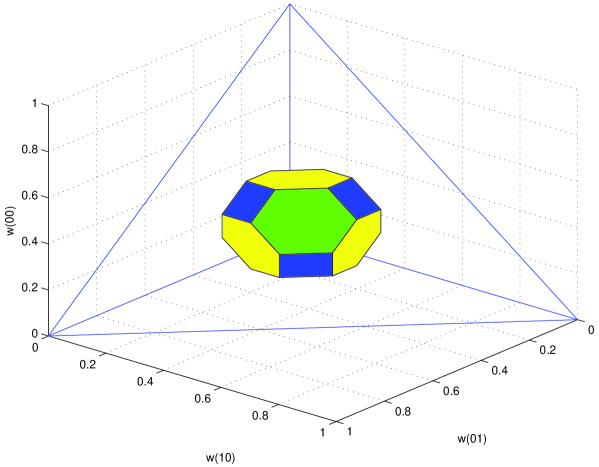
Figure 1: Simplex image of a mixed two qubit state $\lambda_{1}=0.4,\lambda_{2}=0.3,\lambda_{3}=0.2,\lambda_{4}=0.1$.

For a bipartite system of dimension $N_{1}\times N_{2}$, the distinction between factorized and entangled states refers to the behavior under transformations of the factorized group $U(N_{1})\otimes 1+1\otimes U(N_{2})$. We call a state factorized, if the density matrix is

$$\rho=\rho^{(1)}\otimes\rho^{(2)},$$

and classically correlated, if

$$\rho=\sum_{k=1}^{n}c_{k}\rho_{k}^{(1)}\otimes\rho_{k}^{(2)},$$

with $\sum_{k=1}^{n}c_{k}=1$.

Theorem 4.2

The simplex symbol image under $G_{12}=U(N_{1})\otimes 1+1\otimes U(N_{2})$ of a generic factorized or classically correlated state has dimension $\left(N_{1}-1\right)+\left(N_{2}-1\right)$.

Proof : For a classically correlated state, if $n>1$ it is not, in general, possible to find an element of $G_{12}$ diagonalizing $\rho$. Therefore, one has to consider the action of the elementary unitary transformations (102) on a general matrix. $d_{k}\left(\varphi\right)$ does not change the diagonal elements whereas the $g_{ij}\left(\theta\right)$ action for $1\otimes U(N_{2})$ is

$$\begin{array}[]{lll}\sum_{k=1}^{n}c_{k}\left(\rho_{k}^{(1)}\right)_{aa}\otimes\left(\rho_{k}^{(2)}\right)_{ii}&\rightarrow&\begin{array}[]{l}\sum_{k=1}^{n}c_{k}\left(\rho_{k}^{(1)}\right)_{aa}\otimes\left\{\left(\rho_{k}^{(2)}\right)_{ii}\cos^{2}\theta\right.\\ \left.+\left(\rho_{k}^{(2)}\right)_{jj}\sin^{2}\theta-2\mbox{Re}\left(\rho_{k}^{(2)}\right)_{ij}\sin\theta\cos\theta\right\},\end{array}\\ \sum_{k=1}^{n}c_{k}\left(\rho_{k}^{(1)}\right)_{aa}\otimes\left(\rho_{k}^{(2)}\right)_{jj}&\rightarrow&\begin{array}[]{l}\sum_{k=1}^{n}c_{k}\left(\rho_{k}^{(1)}\right)_{aa}\otimes\left\{\left(\rho_{k}^{(2)}\right)_{ii}\sin^{2}\theta\right.\\ \left.+\left(\rho_{k}^{(2)}\right)_{jj}\cos^{2}\theta+2\mbox{Re}\left(\rho_{k}^{(2)}\right)_{ij}\sin\theta\cos\theta\right\},\end{array}\end{array}$$

and for $g_{ij}^{C}\left(\theta\right)$ is

$$\begin{array}[]{lll}\sum_{k=1}^{n}c_{k}\left(\rho_{k}^{(1)}\right)_{aa}\otimes\left(\rho_{k}^{(2)}\right)_{ii}&\rightarrow&\begin{array}[]{l}\sum_{k=1}^{n}c_{k}\left(\rho_{k}^{(1)}\right)_{aa}\otimes\left\{\left(\rho_{k}^{(2)}\right)_{ii}\cos^{2}\theta\right.\\ \left.+\left(\rho_{k}^{(2)}\right)_{jj}\sin^{2}\theta-2\mbox{Im}\left(\rho_{k}^{(2)}\right)_{ij}\sin\theta\cos\theta\right\},\end{array}\\ \sum_{k=1}^{n}c_{k}\left(\rho_{k}^{(1)}\right)_{aa}\otimes\left(\rho_{k}^{(2)}\right)_{jj}&\rightarrow&\begin{array}[]{l}\sum_{k=1}^{n}c_{k}\left(\rho_{k}^{(1)}\right)_{aa}\otimes\left\{\left(\rho_{k}^{(2)}\right)_{ii}\sin^{2}\theta\right.\\ \left.+\left(\rho_{k}^{(2)}\right)_{jj}\cos^{2}\theta+2\mbox{Im}\left(\rho_{k}^{(2)}\right)_{ij}\sin\theta\cos\theta\right\}.\end{array}\end{array}$$

For generic $\rho$ matrices, $U(N_{1})\otimes 1$ and $1\otimes U(N_{2})$ operate independently, therefore, infinitesimal transformations explore $\left(N_{1}-1\right)+\left(N_{2}-1\right)$ independent directions. $\Box$

The generalization to classically correlated multipartite systems is immediate, implying that the image dimension under $\sum_{i}1\otimes\cdots\otimes U(N_{i})\otimes\cdots\otimes 1$ is $\sum_{i}\left(N_{i}-1\right)$.

As an example, we compute explicitly the equation for the two-dimensional surface image in the two-qubit case for a factorized state. In this case, one has to consider mappings from $U(2)\otimes 1+1\otimes U(2)$ to the simplex.

Let $\rho=\rho_{1}\otimes\rho_{2}$. Here, without loosing generality, $\rho$ may be considered as diagonal. Then

$$\Big{(}u(a)\otimes 1+1\otimes u^{\prime}(b)\Big{)}^{\dagger}\left(\rho_{1}\otimes\rho_{2}\right)\Big{(}u(a)\otimes 1+1\otimes u^{\prime}(b)\Big{)}$$

is

$$\left(\begin{array}[]{cc}\left|a_{11}\right|^{2}\lambda_{1}+\left|a_{21}\right|^{2}\lambda_{2}&\ldots\\ \ldots&\left|a_{12}\right|^{2}\lambda_{1}+\left|a_{22}\right|^{2}\lambda_{2}\end{array}\right)$$

$$\otimes\left(\begin{array}[]{cc}\left|b_{11}\right|^{2}\mu_{1}+\left|b_{21}\right|^{2}\mu_{2}&\ldots\\ \ldots&\left|b_{12}\right|^{2}\mu_{1}+\left|b_{22}\right|^{2}\mu_{2}\end{array}\right).$$

Hence

$$w\left(m_{1},m_{2};u(a)\otimes 1+1\otimes u^{\prime}(b)\right)$$

is

$$\begin{array}[]{lll}w\left(00\right)&=&\left(\lambda_{1}\cos^{2}\frac{\theta}{2}+\lambda_{2}\sin^{2}\frac{\theta}{2}\right)\left(\mu_{1}\cos^{2}\frac{\alpha}{2}+\mu_{2}\sin^{2}\frac{\alpha}{2}\right),\\ w\left(01\right)&=&\left(\lambda_{1}\cos^{2}\frac{\theta}{2}+\lambda_{2}\sin^{2}\frac{\theta}{2}\right)\left(\mu_{1}\sin^{2}\frac{\alpha}{2}+\mu_{2}\cos^{2}\frac{\alpha}{2}\right),\\ w\left(10\right)&=&\left(\lambda_{1}\sin^{2}\frac{\theta}{2}+\lambda_{2}\cos^{2}\frac{\theta}{2}\right)\left(\mu_{1}\cos^{2}\frac{\alpha}{2}+\mu_{2}\sin^{2}\frac{\alpha}{2}\right),\\ w\left(11\right)&=&\left(\lambda_{1}\sin^{2}\frac{\theta}{2}+\lambda_{2}\cos^{2}\frac{\theta}{2}\right)\left(\mu_{1}\sin^{2}\frac{\alpha}{2}+\mu_{2}\cos^{2}\frac{\alpha}{2}\right),\end{array}$$

implying

$$w\left(10\right)=\frac{w\left(00\right)}{w\left(01\right)+w\left(00\right)}-w\left(00\right).$$

Figure 2 shows this two-dimensional surface in the 3-dimensional simplex.

For a pure state, this would be the image of the $U(2)\otimes 1+1\otimes U(2)$ group.

For a mixed state, the image is the intersection of the surface with the spanned volume, as in Fig. 1.

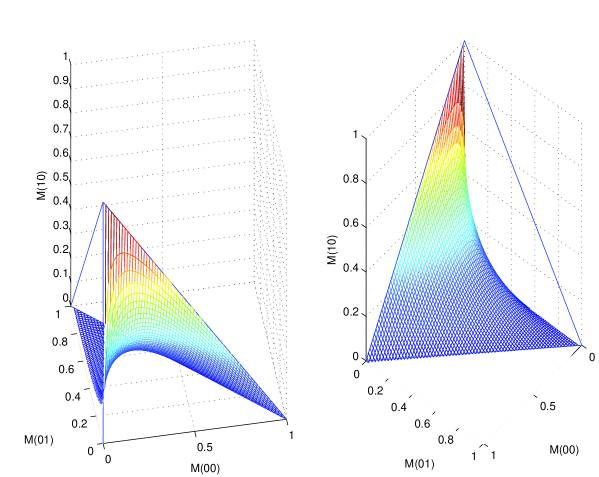
Figure 2: The two-dimensional surface image of $U(2)\otimes 1+1\otimes U(2)$ in the two-qubit case for a factorized pure state.

Theorem 4.2 suggests a notion of geometric correlation, namely,

Definition 4.1

A state of a multipartite system is called geometrically correlated if the symbol image under $\sum_{i}1\otimes\cdots\otimes U(N_{i})\otimes\cdots\otimes 1$ has dimension less than $\sum_{i}\left(N_{i}-1\right)$.

Deviations from geometrical genericity occur when the systems are entangled or the density matrix has special symmetry properties.

As an example, consider the entangled state

$$c_{0}\mid 00\rangle+c1\mid 11\rangle.$$

A simple computation shows that the image under $U(2)\otimes 1+1\otimes U(2)$ is defined by

$$\begin{array}[]{lll}\frac{w\left(00\right)}{\left|c_{0}\right|^{2}}&=&\frac{w\left(11\right)}{\left|c1\right|^{2}},\\ \frac{w\left(10\right)}{c_{1}c_{0}^{*}}&=&\frac{w\left(01\right)}{c_{0}c_{1}^{*}},\end{array}$$

implying that the image is one-dimensional (Figure 3)

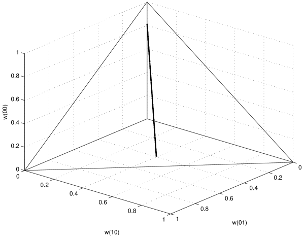
Figure 3: The simplex image of an entangled state.

However, the dimension reduction of the image of $U(2)\otimes 1+1\otimes U(2)$ does not coincide with the notion of entanglement. As an example, consider the Werner state

$$\rho_{W}=\frac{1}{4}\left(\begin{array}[]{llll}1-q&0&0&0\\ 0&1+q&-2q&0\\ 0&-2q&1+q&0\\ 0&0&0&1-q\end{array}\right),$$

$q\leq 1$, which is known to be entangled only for $q>\frac{1}{3}$. In this case, because of the highly symmetric nature of the state, the orbit of the tomgraphic symbol is the same both for $U(2)\otimes 1$ and $1\otimes U(2)$, namely,

$$w=\frac{1}{4}\left(\begin{array}[]{l}\left(1-q\right)\cos^{2}\theta+\left(1+q\right)\sin^{2}\theta\\ \left(1+q\right)\cos^{2}\theta+\left(1-q\right)\sin^{2}\theta\\ \left(1+q\right)\cos^{2}\theta+\left(1-q\right)\sin^{2}\theta\\ \left(1-q\right)\cos^{2}\theta+\left(1+q\right)\sin^{2}\theta\end{array}\right),$$

implying that the image is always one-dimensional.

Incidentally, Peres separability criterium [34] applied to the partial transpose

$$\rho_{W}^{t_{B}}=\frac{1}{4}\left(\begin{array}[]{llll}1-q&0&0&-2q\\ 0&1+q&0&0\\ 0&0&1+q&0\\ -2q&0&0&1-q\end{array}\right)$$

expressed in tomographic operator symbols would be

$$\sum_{\left\{m_{i}\right\}}\left|w_{\rho_{W}^{t_{B}}}(\left\{m_{i}\right\},u)\right|=1\hskip 56.9055pt\forall u,$$

the state being entangled when there is an $u$ for which this identity is violated.

5 Measurements and generalized measurements

In the standard quantum formulation, measurements are realized by von Neumann “instruments” which are orthogonal projectors $\hat{P}_{j}$ onto eigenstates of the variables being measured. The projectors applied to the pure state $\mid\psi\rangle$ yield

$$\mid\psi\rangle_{j}=\hat{P}_{j}\mid\psi\rangle,\quad\hat{P}_{j}=\mid\psi_{j}\rangle\langle\psi_{j}\mid,$$ (106)

or in terms of density matrix $\mid\psi\rangle\langle\psi\mid$, one has the result

$$\mid\psi\rangle_{j}\,{}_{j}\langle\psi\mid=\hat{P}_{j}\mid\psi\rangle\langle\psi\mid\hat{P}_{j}=\hat{P}_{j}\hat{\rho}_{\psi}\hat{P}_{j}=|\langle\psi\mid\psi_{j}\rangle|^{2}\mid\psi_{j}\rangle\langle\psi_{j}\mid.$$ (107)

For a mixed state $\hat{\rho}$, the measurement provides the state density operator after measurement

$$\hat{\rho}_{j}=\hat{P}_{j}\hat{\rho}\hat{P}_{j}.$$ (108)

Generalized measurements use positive operator-valued measures (POVM), that is, positive operators $\hat{P}_{k}$ with the property

$$\sum_{k}\hat{P}_{k}=\hat{1},$$ (109)

the index $k$ being either discrete or continuous. In the latter case, one has an integration in (109).

Within the framework of operator symbols and star-products, instead of (108), we have after the measurement a symbol for the density operator of the state

$$f_{\hat{\rho}_{j}}(\mathbf{x})=f_{\hat{P}_{j}}(\mathbf{x})\star f_{\hat{\rho}}(\mathbf{x})\star f_{\hat{P}_{j}}(\mathbf{x}),$$ (110)

$f_{\rho}(\mathbf{x})$ being the symbol of the density operator of measurable state and $f_{\hat{P}_{j}}(\mathbf{x})$ the symbol of the instrument.

In the tomographic probability representation, the result of measurements is described by a map of the probability distributions, namely,

$$w_{j}(X,\mu,\nu)=w_{\hat{P}_{j}}(X,\mu,\nu)\star w(X,\mu,\nu)\star w_{\hat{P}_{j}}(X,\mu,\nu),$$ (111)

with the kernel of the star-product of tomograms given by Eq. (46).

For the case of spin (or unitary spin) tomograms, the linear map of tomographic-probability distributions is realized by the formula

$$w_{j}(m,\vec{n})=w_{\hat{P}_{j}}(m,\vec{n})\star w(m,\vec{n})\star w_{\hat{P}_{j}}(m,\vec{n}),$$ (112)

the kernel of the star-product being given by Eq. (LABEL:eq.26a). One sees that, in the probability representation, the process of measurement, both with von Neumann instruments and with POVM, is described by a map of points in the simplex.

6 Time evolution of quantum states and superoperators

In the standard representation of quantum mechanics, states (state vectors $\mid\psi,t\rangle$ or density operators $\hat{\rho}(t)$) of closed system evolve according to unitary change

$$\mid\psi,t\rangle=\hat{U}(t)\mid\psi,0\rangle,$$ (113)

or

$$\hat{\rho}(t)=\hat{U}(t)\hat{\rho}(0)\hat{U}^{\dagger}(t).$$ (114)

This evolution is a solution to Schrödinger or von Neumann equations

$$\frac{\partial}{\partial t}\hat{\rho}(t)+i[\hat{H},\rho(t)]=0,$$ (115)

$\hat{H}$ being the Hamiltonian of the system.

The evolution can be cast into operator symbol form.

Let $f_{A}(\mathbf{{x})}$ be the symbol of an operator $\hat{A}$. We do not specify at the moment what kind of symbols are used, considering them as generic ones with quantizer–dequantizer pair $\hat{D}(\mathbf{{x})}$, $\hat{U}(\mathbf{{x})}$. Then, the operator equation (115) for density operator reads

$$\frac{\partial}{\partial t}w_{\rho}(\mathbf{x},t)+i\Big{(}f_{H}(\mathbf{x},t)\star w_{\rho}(\mathbf{x},t)-w_{\rho}(\mathbf{x},t)\star f_{H}(\mathbf{x},t)\Big{)}=0.$$ (116)

We denote the symbol of the density operator $\hat{\rho}(t)$ by $w_{\rho}(\mathbf{x},t)$. The solution of Eq. (116) has a form corresponding to (114)

$$w_{\rho}(\mathbf{x},t)=f_{U}(\mathbf{x},t)\star w_{\rho}(\mathbf{x},0)\star f_{U^{\dagger}}(\mathbf{x},t).$$ (117)

One can rewrite the solution (114) as a superoperator $L$ acting in a linear space of operators, namely,

$$\hat{\rho}(t)=L(t)\hat{\rho}(0).$$ (118)

In matrix form, Eq. (118) reads

$$\hat{\rho}(t)_{\alpha\beta}=\sum_{\gamma\delta}L(t)_{\alpha\beta\,\gamma\delta}\hat{\rho}(0)_{\gamma\delta}.$$ (119)

For unitary evolution, the superoperator is expressed in terms of unitary matrix $U(t)$ as a tensor product

$$L(t)_{\alpha\beta\,\gamma\delta}=U(t)_{\alpha\beta}\otimes U^{*}(t)_{\gamma\delta}.$$ (120)

One rewrites the solution (117) for the symbol introducing the propagator

$$w_{\rho}(\mathbf{x},t)=\int\Pi(\mathbf{x},\mathbf{y},t)w_{\rho}(\mathbf{y},0)\,d\mathbf{y}.$$ (121)

For the unitary evolution (114), the propagator reads

$$\Pi(\mathbf{x}_{1},\mathbf{x}_{2},t)=\int k(\mathbf{y}_{1},\mathbf{x}_{2},\mathbf{y}_{2},\mathbf{x}_{1})f_{U(t)}(\mathbf{y}_{1})f_{U^{\dagger}(t)}(\mathbf{y}_{2})\,d\mathbf{y}_{1}\,d\mathbf{y}_{2},$$ (122)

where

$$k(\mathbf{y}_{1},\mathbf{x}_{2},\mathbf{y}_{2},\mathbf{x}_{1})=\int K(\mathbf{y}_{1},\mathbf{x}_{2},\mathbf{x}_{3})K(\mathbf{x}_{3},\mathbf{y}_{2},\mathbf{x}_{1})\,d\mathbf{x}_{3}.$$

The kernels under the integral are given by Eq. (82).

In the case of superoperators describing the evolution of an open system [35, 36]

$$\hat{\rho}(0)\rightarrow\hat{\rho}(t)=\sum_{s}\hat{V}_{s}(t)\hat{\rho}(0)\hat{V}_{s}^{\dagger}(t),\qquad\sum_{s}\hat{V}_{s}^{\dagger}(t)\hat{V}_{s}(t)=1,$$ (123)

the propagator reads

$$\Pi(\mathbf{x},\mathbf{y},t)=\int\sum_{s}f_{V(t)}^{(s)}(\mathbf{y}_{1})f_{V^{\dagger}(t)}^{(s)}(\mathbf{y}_{2})k(\mathbf{y}_{1},\mathbf{y},\mathbf{y}_{2},\mathbf{x})\,d\mathbf{y}_{1}\,d\mathbf{y}_{2}.$$ (124)

The propagator corresponds to a superoperator, which in matrix form reads

$$\Big{(}L(t)\Big{)}_{\alpha\beta\,\gamma\delta}=\sum_{s}(V_{s})_{\alpha\beta}\otimes(V_{s}^{*})_{\gamma\delta}.$$ (125)

For the case of continuous variables and symplectic tomograms, Eq. (116) takes the form of a deformed Boltzman equation for the probability distribution.

For unitary spin tomograms, one has

$$w_{\rho}(m,u,t)=w_{\rho}\left(m,U^{\dagger}(t)u,0\right),$$ (126)

the unitary evolution matrix being determined by an Hamiltonian matrix

$$U(t)=e^{-itH}.$$ (127)

This means that the unitary spin tomogram, a function on the unitary group, evolves according to the regular representation of the unitary group. This means that the partial differential equation for the infinitesimal action is the standard equation for matrix elements of the regular representation, that is,

$$i\frac{\partial}{\partial t}w(m,u,t)=\sum_{ik}\Big{(}H_{ik}\hat{L}_{ik}(u)\Big{)}w(m,u,t),$$

$H_{ik}$ being the Hamiltonian hermitian matrix and $\hat{L}_{ik}(u)$ the infinitesimal hermitian first-order differential operators of the left regular representation of the unitary group in the chosen group parametrization.

7 Examples of quantum channels

In this section, we consider the unitary spin representation of some typical quantum channels.

7.1 Depolarizing channel

Consider bit flip, phase flip and both with equal probability

$$\begin{array}[]{l}\mid\psi\rangle\rightarrow\sigma_{1}\mid\psi\rangle=\left(\begin{array}[]{ll}0&1\\ 1&0\end{array}\right)\mid\psi\rangle,\\ \mid\psi\rangle\rightarrow\sigma_{3}\mid\psi\rangle=\left(\begin{array}[]{ll}1&0\\ 0&-1\end{array}\right)\mid\psi\rangle,\\ \mid\psi\rangle\rightarrow\sigma_{2}\mid\psi\rangle=\left(\begin{array}[]{ll}0&-i\\ i&0\end{array}\right)\mid\psi\rangle.\end{array}$$

The Kraus representation is

$$\rho_{0}\rightarrow\rho=\left(1-p\right)\rho+\frac{p}{3}\left(\sigma_{1}\rho\sigma_{1}+\sigma_{2}\rho\sigma_{2}+\sigma_{3}\rho\sigma_{3}\right).$$

For the unitary spin symbol representation, choosing the axis one has

$$\rho_{0}=\frac{1}{2}(1+\sigma_{3})$$

and with an arbitrary unitary group element

$$u=\cos\frac{\theta}{2}-i\sigma\cdot n\sin\frac{\theta}{2}$$

one obtains

$$\begin{array}[]{lll}w\left(+,u\right)&=&\frac{1}{2}\left\{1+\left(1-\frac{4}{3}p\right)\left(\cos^{2}\frac{\theta}{2}+\left(2n_{3}^{2}-1\right)\sin^{2}\frac{\theta}{2}\right)\right\},\\ w\left(-,u\right)&=&\frac{1}{2}\left\{1-\left(1-\frac{4}{3}p\right)\left(\cos^{2}\frac{\theta}{2}+\left(2n_{3}^{2}-1\right)\sin^{2}\frac{\theta}{2}\right)\right\}.\end{array}$$

When $p\rightarrow 1$ the image in the simplex contracts to a segment between $\left(\frac{2}{3},\frac{1}{3}\right)$ and $\left(\frac{1}{3},\frac{2}{3}\right)$.

7.2 Phase-damping channel

$$\begin{array}[]{l}\mid 0\rangle\mid 0\rangle_{E}\rightarrow\sqrt{1-p}\mid 0\rangle\mid 0\rangle_{E}+\sqrt{p}\mid 0\rangle\mid 1\rangle_{E},\\ \mid 1\rangle\mid 0\rangle_{E}\rightarrow\sqrt{1-p}\mid 1\rangle\mid 0\rangle_{E}+\sqrt{p}\mid 1\rangle\mid 2\rangle_{E}.\end{array}$$

The Kraus representation is

$$\rho_{0}\rightarrow\rho=\sum_{\mu}K_{\mu}\rho_{0}K_{\mu}^{\dagger},$$

with

$$K_{0} = \sqrt{1-p}\left(\begin{array}[]{ll}1&0\\ 0&0\end{array}\right),\qquad K_{1}=\sqrt{p}\left(\begin{array}[]{ll}1&0\\ 0&0\end{array}\right),$$

$$\qquad K_{2} = \sqrt{p}\left(\begin{array}[]{ll}0&0\\ 0&1\end{array}\right).$$

For the unitary spin symbol representation, consider the example

$$\mid\psi\rangle=\frac{1}{\sqrt{2}}\left(\mid 0\rangle+\mid 1\rangle\right),$$

$$\rho_{0}=\left(\begin{array}[]{ll}\frac{1}{2}&\frac{1}{2}\\ \frac{1}{2}&\frac{1}{2}\end{array}\right).$$

Then

$$\begin{array}[]{lll}w\left(+,u\right)&=&\frac{1}{2}\left\{1+2\left(1-p\right)\sin\frac{\theta}{2}\left(n_{2}\cos\frac{\theta}{2}+n_{1}n_{3}\sin\frac{\theta}{2}\right)\right\},\\ w\left(-,u\right)&=&\frac{1}{2}\left\{1-2\left(1-p\right)\sin\frac{\theta}{2}\left(n_{2}\cos\frac{\theta}{2}+n_{1}n_{3}\sin\frac{\theta}{2}\right)\right\}.\end{array}$$

and when $p\rightarrow 1$ the image in the simplex contracts to a point.

7.3 Amplitude damping channel

$$\begin{array}[]{l}\left|0\right\rangle\left|0\right\rangle_{E}\rightarrow\left|0\right\rangle\left|0\right\rangle_{E},\\ \left|1\right\rangle\left|0\right\rangle_{E}\rightarrow\sqrt{1-p}\left|1\right\rangle\left|0\right\rangle_{E}+\sqrt{p}\left|0\right\rangle\left|1\right\rangle_{E}.\end{array}$$

The Kraus representation is

$$\rho_{0}\rightarrow\rho=\sum_{\mu}K_{\mu}\rho_{0}K_{\mu}^{\dagger},$$

with

$$K_{0}=\left(\begin{array}[]{ll}1&0\\ 0&\sqrt{1-p}\end{array}\right),\qquad K_{1}=\left(\begin{array}[]{ll}0&\sqrt{p}\\ 0&0\end{array}\right).$$

For the unitary spin representation, consider an excited initial state

$$\mid\psi\rangle=\mid 1\rangle,$$

$$\rho_{0}=\left(\begin{array}[]{ll}0&0\\ 0&1\end{array}\right).$$

Then

$$\begin{array}[]{lll}w\left(+,u\right)&=&p\cos^{2}\frac{\theta}{2}+\left(pn_{3}^{2}+\left(1-p\right)\left(1-n_{3}^{2}\right)\right)\sin^{2}\frac{\theta}{2}\,,\\ w\left(-,u\right)&=&\left(1-p\right)\cos^{2}\frac{\theta}{2}+\left(\left(1-p\right)n_{3}^{2}+p\left(1-n_{3}^{2}\right)\right)\sin^{2}\frac{\theta}{2}\,.\end{array}$$

When $p$ varies from $0$ to $1$, the image in the simplex first contracts to a point $\left(p=\frac{1}{2}\right)$ and then expands again to the whole simplex when $p\rightarrow 1$.

The operator symbols being functions on the rotation or unitary groups are highly redudant descriptions of qudit states. As expected from the number of independent parameters in the density matrix, also here $\left(d^{2}-1\right)$ numbers are enough to characterize a $d-$dimensional qudit. This is easy to check. Consider the operator symbol (92) for an arbitrary $d-$dimensional density matrix $\rho$. A general $\rho$ may be diagonalized by of $d\left(d-1\right)$ independent unitary transformations and this, together with the $\left(d-1\right)$ independent diagonal elements, gives the desired result.

Alternatively we may consider $\left(d+1\right)$ independent elements of the unitary group and compute the associated operator symbols. Then, the qudit state would be described by their diagonal elements. Therefore, a discrete quantum state (qudit) is coded by $\left(d+1\right)$ probability distributions.

For each $u$ in the group, the elements in the operator symbol $w(\left\{m_{i}\right\},u)$ are the probabilities to obtain the values $\left\{m_{i}\right\}$ in a measurement of the quantum state $\rho$ by an apparatus oriented along $u$. Therefore the problem of reconstructing the state $\rho$ from the set of $\left(d+1\right)\left(d-1\right)$ operator symbol elements is identical to the reconstruction of the density matrix of a spin through Stern-Gerlach experiments, already discussed in the literature[38] [39] [40].

8 Entropies

8.1 Operator symbol entropies

The tomographic operator symbols satisfy

$$\sum_{\left\{m_{i}\right\}}w(\left\{m_{i}\right\},u)=1,$$

therefore, they are probability distributions $\forall u$.

One defines the operator symbol entropy by

$$H_{u}=-\sum_{\left\{m_{i}\right\}}w(\left\{m_{i}\right\},u)\ln w(\left\{m_{i}\right\},u)$$

and the operator symbol Rényi entropies by

$$R_{u}=\frac{1}{1-q}\ln\left(\sum_{\left\{m_{i}\right\}}w(\left\{m_{i}\right\},u)^{q}\right).$$

Likewise, we may define the operator symbol relative q-entropy by

$$H_{q}(w_{1}(u)|w_{2}(u))=-\sum_{\left\{m_{i}\right\}}w_{1}(\left\{m_{i}\right\},u)\ln_{q}\frac{w_{2}(\left\{m_{i}\right\},u)}{w_{1}(\left\{m_{i}\right\},u)},$$ (130)

with

$$\ln_{q}x=\frac{x^{1-q}-1}{1-q}\,,\quad x>0,\quad q>0,\quad\ln_{q\rightarrow 1}x=\ln x.$$ (131)

Because the operator symbols $w\left(\left\{m_{i}\right\},u\right)$ are probability distributions, they inherit all the known properties of nonnegativity, additivity, joint convexity, etc. of classical information theory.

The relation of the operator symbol entropies to the von Neumann and the quantum Rényi entropies is given by the following

Theorem 8.1

The von Neumann $S$ and the quantum Rényi $S_{q}$ entropies are the minimum on the unitary group of $H_{u}$ and $R_{u}$.

Proof : From

$$w(\left\{m_{i}\right\},u)=\langle\left\{m_{i}\right\}\mid u^{\dagger}\rho u\mid\left\{m_{i}\right\}\rangle$$ (132)

there is a $u^{*}$ such that $u^{*\dagger}\rho u^{*}$ is a diagonal matrix $\left\{\lambda_{1},\lambda_{2},\ldots\lambda_{n}\right\}$. Then

$$H_{u^{*}}=-\mbox{Tr}\,\rho\ln\rho=S=\mbox{von\,\,Neumann\,\, entropy}$$

For any other $u$, the diagonal elements in (132) are convex linear combinations of $\left\{\lambda_{1},\lambda_{2},...\lambda_{n}\right\}$. By convexity of $w(\left\{m_{i}\right\},u)\ln w(\left\{m_{i}\right\},u)$ the result follows for the von Neumann entropy.

The operator symbol Rényi entropy is not a sum of concave functions. However, the following function is,

$$T_{u}=-\sum_{\left\{m_{i}\right\}}w(\left\{m_{i}\right\},u)^{q}\ln_{q}w(\left\{m_{i}\right\},u)$$

called the Tsallis entropy[32] and related to the Rényi[33] entropy by

$$R_{u}=\frac{1}{1-q}\ln\Big{(}1+\left(1-q\right)T_{u}\Big{)}.$$ (133)

The minimum result now applies to $T_{u}$ by concavity and then one checks from (133) that it also holds for $R_{u}$. Therefore $R_{u^{*}}=R_{u}\min$ coincides with the quantum Rényi entropy

$$S_{q}=\frac{1}{1-q}\ln(\mbox{Tr}\,\rho^{q}).$$

$\Box$

The entropy $H_{u}$ varies from the minimum, which is von Neumann entropy, to a maximum for the most random distribution. For each given state $\rho$, one can also define the integral entropies

$$H_{\rho}=\int H_{u}\,du,\qquad R_{\rho}=\int R(u)\,du,\qquad H_{q}(\rho_{1},\rho_{2})=\int H_{q}(w_{1}(u)|w_{2}(u))\,du,$$

where $du$ is the invariant Haar measure on unitary group.

In some cases, the properties of the von Neumann entropy may be derived as simple consequences of the classical-like properties of the operator symbol entropies. For example:

Subadditivity: $S_{12}\leq S_{1}+S_{2}$

Consider a two-partite system with density matrix $\rho_{12}$

$$w(m_{1},m_{2},u)=\langle m_{1}m_{2}\mid u^{\dagger}\rho_{12}u\mid m_{1}m_{2}\rangle,$$

$u$ being a $(2j_{1}+1)(2j_{2}+1)\times(2j_{1}+1)(2j_{2}+1)$ unitary matrix

$$H_{u}\left(12\right)=-\sum_{m_{1}m_{2}}w(m_{1},m_{2},u)\ln w(m_{1},m_{2},u)$$

From the reduced symbols and density matrices

$$w(m_{1},u)=\sum_{m_{2}}w(m_{1},m_{2},u),$$

$$(\rho_{1})_{m_{1}m_{1}^{\prime}}=\sum_{m_{2}}(\rho_{12})_{m_{1}m_{2}m_{1}^{\prime}m_{2}},$$

one writes the reduced symbol entropies

$$H_{u}(1)=-\sum_{m_{1}}w(m_{1},u)\ln\,w(m_{1},u),$$

$$H_{u}(2)=-\sum_{m_{2}}w(m_{2},u)\ln\,w(m_{2},u).$$

For each fixed $u$, the tomographic symbols are ordinary probability distributions. Therefore, by the subadditivity of classical entropy,

$$H_{u}(12)\leq H_{u}(1)+H_{u}(2).$$

In particular, this is true for the group element in $u^{*}\in U_{j_{1}}\otimes U_{j2}$ that diagonalizes the reduced density matrices $\rho_{1}$ and $\rho_{2}$. Therefore,

$$H_{u^{*}}(12)\leq S_{1}+S_{2}.$$

But, by the minimum property,

$$S_{12}\leq S_{1}+S_{2}.$$

Thus subadditivity for the von Neumann entropy is a consequence of subadditivity for the operator symbol entropies.

The situation concerning strong subadditivity is different. Strong subadditivity also holds, of course, for the operator symbol entropies for any $u$

$$H_{u}(123)+H_{u}(2)\leq H_{u}(12)+H_{u}(23),$$ (134)

but the corresponding relation for the von Neumann entropy is not a direct consequence of (134). The strong subadditivity[37] for the von Neumann entropy

$$S\left(123\right)+S\left(2\right)\leq S\left(12\right)+S\left(23\right)$$ (135)

expressed in operator symbol entropies would be

$$H_{u_{1}^{*}}(123)+H_{u_{2}^{*}}(2)\leq H_{u_{3}^{*}}(12)+H_{u_{4}^{*}}(23)$$

where $u_{1}^{*}\in U\left(123\right),u_{2}^{*}\in 1\otimes U(2)\otimes 1,u_{3}^{*}\in U\left(12\right)\otimes 1,u_{4}^{*}\in 1\otimes U(23)$ are the different group elements that diagonalize the respective subspaces. Therefore strong subadditivity for the von Neumann entropy (135) and strong subadditivity for the operator symbol entropies (134) are independent properties. On the other hand, because of the invertible relation (78) between the operator symbols and the density matrix, Eq.(134) contains in fact a family of new inequalities for functionals of the density matrix.

9 Conclusions

To conclude we summarize the main results of this work :

(i) A unified formulation for an operator symbol formulation of standard quantum theory.

(ii) A (spin) operator symbol framework to deal with quantum information problems.

(iii) Evolution equations for qudit operator symbols are written in the form of first-order partial differential equations with generators describing the left regular representation of the unitary group.

(iv) Measurements are discussed in the operator-symbol representation of qudits.

(v) A geometric interpretation of (spin) operator symbols of qudit states as maps of the unitary group to the simplex.

(vi) In view of the probability nature of the operator symbols, the corresponding entropies inherit the properties of classical information theory. Some of the properties of the von Neumann entropy and quantum Rényi entropy are direct consequences of these properties. On the other hand the properties of the operator symbol entropies also imply new relations for functionals of the density matrix.

References

• [1] Stratonovich R.L., Zh. Γ‰ksp. Teor. Fiz. 31 (1956) 1012 [Sov. Phys. JETP 4 (1975) 891]
• [2] Bayen F., Flato M., Fronsdal C., Lichnerovicz A. and Sternheimer D., Lett. Math. Phys. 1 (1975) 521
• [3] Wigner E., Phys. Rev., 40 (1932) 749
Weyl H., Z. Phys. 46 (1927) 1
• [4] Moyal J. E., Proc. Cam. Phil. Soc., 45 (1949) 99
• [5] K. E. Cahill and R. J. Glauber; Phys. Rev. 177 (1969) 1882.
• [6] R. J. Glauber; Phys. Rev. 131 (1963) 2766–2788; Phys. Rev. Lett. 10 (1963) 84–86.
• [7] E. C. G. Sudarshan, Phys. Rev. Lett. 10 (1963) 277–279.
• [8] K. Husimi; Proc. Phys. Math. Soc. Jpn, 22 (1940) 264–314.
• [9] Y. Kano; J. Math. Phys. 6 (1965) 1913–1915.
• [10] S. Mancini, V. I. Man’ko and P. Tombesi; J. Mod. Opt. 44 (1997) 2281.
• [11] V. V. Dodonov and V. I. Man’ko, Phys. Lett. A 239 (1997) 335.
• [12] V.I. Man’ko and O.V. Man’ko, JETPΒ 85 (1997) 430.
• [13] O. V. Man’ko, V. I. Man’ko and G. Marmo; J. Phys. A: Math. Gen. 35 (2002) 699.
• [14] O.V. Man’ko, V.I. Man’ko, and G. Marmo, Physica ScriptaΒ 62 (2000) 446.
• [15] S. Mancini, V. I. Man’ko and P. Tombesi; Phys. Lett. A 213 (1996) 1.
• [16] S. Mancini, V. I. Man’ko and P. Tombesi; Found. Phys. 27 (1997) 801.
• [17] O.V. Man’ko and V.I. Man’ko, J. Russ. Laser Res.Β 25 (2004) 115.
• [18] L. D. Landau, Z. Phys. 45 (1927) 430
• [19] J.Β vonΒ Neumann, Mathematische Grundlagen der Quantummechanik, Springer, Berlin (1932).
• [20] J.Β vonΒ Neumann,Β GΓΆttingenische Nachrichten, 11 (Nov.Β 1927), S.Β 245–272.
• [21] V. I. Man’ko and R. Vilela Mendes, Physica D 145 (2000) 230.
• [22] A. S. Arkhipov and Yu. E. Lozovik; Phys. Lett. A 319 (2003) 217.
• [23] M. A. Man’ko, V. I. Man’ko and R. Vilela Mendes; J. Phys. A: Math. Gen. 34 (2001) 8321.
• [24] G. M. D’Ariano, S. Mancini, V. I. Ma’ko and P. Tombesi; J. Opt. B: Quantum Semiclass. Opt. 8 (1996) 1017.
• [25] V. I. Man’ko and R. Vilela Mendes; Phys. Lett. A, 263 (1999) 53–59.
• [26] V. A. Andreev, O. V. Man’ko, V. I. Man’ko and S. S. Safonov; J. Russ. Laser Res. 19 (1998) 340.
• [27] A.B. Klimov, O.V. Man’ko, V.I. Man’ko, Yu. F. Smirnov and V.N. Tolstoy, J. Phys. A: Math Gen.Β 35 (2002) 6101.
• [28] O. CastaΓ±os, R. Lopez-PeΓ±a, M. A. Man’ko, and V. I. Man’ko, J. Phys. A: Math Gen., 36 (2003) 4677.
• [29] D. A. Varshalovich, A. N. Moskalev, and V. K. Khersonsky, Theory of Angular Momentum, World Scientific, Singapore 1998.
• [30] V.I. Man’ko, G. Marmo, E.C.G. Sudarshan and F. Zaccaria, Phys. Lett. A 327 (2004) 353.
• [31] C. E. Shannon, Bell Sytems Technical Journal 27 (1948) 379
• [32] C. Tsallis et al., in: Nonextensive Statistical Mechanics and Its Applications, ed. by S. Abe and Y. Okamoto (Springer, Heidelberg, 2001)
• [33] A. RΓ¨nyi, Probability Theory (North-Holland, Amsterdam, 1970)
• [34] A. Peres;Β Phys. Rev. Lett. 77 (1996) 1413
• [35] E.C.G. Sudarshan, P.M. Mathews and J. Rau, Phys. Rev. 121 (1961) 920
• [36] K. Kraus, States, Effects and Operations: Fundamental Notion of Quantum Theory, in: Lecture Notes in Physics, Springer, Berlin, Vol. 190 (1983)
• [37] E. H. Lieb and M. B. Ruskai; J. Mat. Phys. 14 (1973) 1938.
• [38] R. G. Newton and B. Young; Ann. Phys. (NY) 49 (1968) 393.
• [39] J.-P. Amiet and S. Weigert; J. Phys. A: Math. Gen. 32 (1999) L269.
• [40] J.-P. Amiet and S. Weigert; J. Opt. B: Quantum and Semiclass. Opt. 1 (1999) L5.