Geometric phase in open systems: beyond the Markov approximation and weak coupling limit

Abstract

Beyond the quantum Markov approximation and the weak coupling limit, we present a general theory to calculate the geometric phase for open systems with and without conserved energy. As an example, the geometric phase for a two-level system coupling both dephasingly and dissipatively to its environment is calculated. Comparison with the results from quantum trajectory analysis is presented and discussed.

I introduction

Since Berry’s discovery berry84 that a state of a quantum system can acquire a phase of purely geometric origin when the Hamiltonian of the system undergoes a cyclic and adiabatic change, there have been numerous proposals for generalizations, including the geometric phase for nonadiabatic, noncyclic, and nonunitary evolution shapere89 , the geometric phase for mixed states uhlmann86 ; sjoqvist00a , the geometric phase in systems with quantum field driving and vacuum induced effects fuentes02 , as well as the geometric phase in coupled bipartite systemsyi04 .

Recently, the attention has turned to studying geometric phase in open systems, this is motivated by the fact that all realistic system are coupled, at least weakly, to their environment. From the perspective of application, the use of geometric phases in the implementation of fault-tolerant quantum gates zanardi99 ; jones99 ; ekert00 ; falci00 requires the study of geometric phases in more realistic systems. For instance, the system which carries information may decoher from a quantum superposition into statistical mixtures, and this effect, called decoherence, is the most important limiting factor for quantum computing.

The study of geometric phase in open systems may be traced back to 1980s, when Garrison and Wright garrison88 first touched on this issue by describing open system evolution in terms of non-Hermitian Hamiltonian. This is a pure state analysis, so it did not address the problem of geometric phases for mixed states. Toward the geometric phase for mixed states in open systems, the approaches used include solving the master equation of the system fonsera02 ; aguiera03 ; ellinas89 ; gamliel89 ; kamleitner04 , employing a quantum trajectory analysis nazir02 ; carollo03 or Krauss operators marzlin04 , and the perturbative expansions whitney03 ; gaitan98 . Some interesting results were achieved that may be briefly summarized as follows: nonhermitian Hamiltonian lead to a modification of Berry’s phase garrison88 ; whitney03 , stochastically evolving magnetic fields produce both energy shift and broadening gaitan98 , phenomenological weakly dissipative Liouvillians alter Berry’s phase by introducing an imaginary correction ellinas89 or lead to damping and mixing of the density matrix elements gamliel89 . However, almost all these studies are performed for dissipative systems under various approximations, thus the representations are approximately applicable for systems whose energy is not conserved. Quantum trajectory analysis nazir02 ; carollo03 that uses the quantum jump approach is available for open systems with conserved energy. Its starting point, however, is the master equation, a result within the quantum Markov approximation and in the weak coupling limit. Beyond the quantum Markov approximation and the weak coupling limit, the geometric phase of a two-level system with quantum field driving was analyzed yi05 , where the whole system (the two-level system plus the quantum field) was assumed subject to dephasing, the subsystem(two-level system in that paper) may still acquire geometric phase even when the whole system in its pointer states. This is an ideal situation to show the vacuum effects on the geometric phase of the subsystem, as well as the decoherence effects on the geometric phases regardless of its feasibility of experimental realization. However, beyond the Markov approximation and the weak coupling limit, the geometric phase for a dissipative system remains untouched. In this paper, we will deal with the geometric phase in open systems, beyond the Markov approximation and weak coupling limit.

The structure of this paper is organized as follows. In Sec. II the exact solution and calculation of the geometric phase of a system dephasingly coupled to its environment is presented, an example to detail the representation and a discussion on physical realization are given in Sec. III. In Sec. IV, we present an example to show the calculation of geometric phases in dissipative systems. Finally we conclude in Sec.V.

II geometric phase in dephasing systems: general formulation

In this section, we investigate the behavior of geometric phase of a quantum system subject to decoherence. In order to make a comparison with the results from the quantum jump approach, we consider the quantum system without any field driving except the environment. So, it is not directly relevant to our previous studyyi05 . The environment that leads to decoherence may originate form the vacuum fluctuations or the background radiations. We restrict ourselves here to consider the case where the system-environment coupling $H_{I}$ and the free system Hamiltonian $H_{S}$ commute. This is the situation of dephasing and the exact analytical dynamics may be obtained. On the other hand, the evolution of a system with such properties may be described by the master equation when the Markov approximation and the weak coupling assumption apply, this kind of decoherence would not change the geometric phase of the quantum system by the quantum jump approachnazir02 ; carollo03 . However, as you will see, this is not the case from the viewpoint of interferometry considered in this paper.

We consider a situation described by a Hamiltonian of the form

$$H=H_{S}+H_{B}+H_{I},$$ (1)

where $H_{S}$ describes the free Hamiltonian of the system, $H_{B}$ stands for the Hamiltonian of the environment, and $H_{I}$ represents the system-environment couplings. The environment and the system Hamiltonian may be taken arbitrary but with constraints $[H_{S},H_{I}]=0$. Let us suppose that the interaction Hamiltonian $H_{I}$ has the form (setting $\hbar=1$)

$$H_{I}=\sum_{m}X_{m}(\Gamma_{m}^{\dagger}+\Gamma_{m}),$$ (2)

where the $X_{m},(m=1,2,...,M)$ are the system operators satisfying $[H_{S},X_{m}]=0,$ and the $\Gamma_{m}$ represent environment operators that may take any form in general. Commutation relation $[H_{S},X_{m}]=0$ enables us to write the time evolution operator for the whole systems(system+environment) as

$$U(t)=e^{-iHt}=e^{-iH_{S}t}\sum_{m}U_{m}(t)|E_{m}\rangle\langle E_{m}|$$ (3)

with $U_{m}(t)$, a function of environment operators satisfying

$$i\frac{\partial}{\partial t}U_{m}(t) = H_{e,m}U_{m}(t),$$

$$H_{e,m} = H_{B}+\sum_{n}e_{n}^{m}(\Gamma_{n}+\Gamma_{n}^{\dagger}).$$ (4)

Here, $|E_{m}\rangle$ stands for the eigenstate of $H_{S}$ with eigenvalue $E_{m}$note1 , while $e_{n}^{m}$ denotes the eigenvalue of $X_{n}$ corresponding to eigenstate $|E_{m}\rangle$. For a specific $\Gamma_{m}$, $U_{m}(t)$ may be expressed in a factorized form, which will be shown later through the spin-boson model. Furthermore, we assume that the environment and the system are initially independent, such that the total density operator factorizes into a direct product,

$$\rho(0)=\rho_{S}(0)\otimes\rho_{B}(0)=$$

$$\sum_{mn}\rho_{mn}(0)|E_{m}\rangle\langle E_{n}|\otimes\rho_{B}(0).$$ (5)

At time $t$, the reduced density operator of the system is given by

$$\rho_{S}(t) = \mbox{Tr}_{B}(U(t)\rho_{S}(0)\otimes\rho_{B}(0)U^{\dagger}(t))$$ (6)

$$\equiv \sum_{mn}\rho_{mn}(0)e^{-i(E_{m}-E_{n})t}|E_{m}\rangle\langle E_{n}|F_{mn}(t),$$

where $F_{mn}(t)$ is defined as $\mbox{Tr}_{B}[U_{m}(t)\rho_{B}(0)U_{n}^{\dagger}(t)].$ Eq.(6) shows that the diagonal elements of the reduced density matrix $\rho_{mm}$ are time-independent, while the off-diagonal elements evolve with time involving contributions from the environment-system couplings, it at most cases would lead to decaying in the off-diagonal elements, and eventually results in vanishing of these matrix elements. Now we turn to study the geometric phase of the open system. For open systems, the states in general are not pure and the evolution of the system is not unitary. For non-unitary evolutions, the geometric phase can be calculated as follows. First, solve the eigenvalue problem for the reduced density matrix $\rho(t)$ and obtain its eigenvalues $\varepsilon_{k}(t)$ as well as the corresponding eigenvectors $|\psi_{k}(t)\rangle;$ secondly, substitute $\varepsilon_{k}(t)$ and $|\psi_{k}(t)\rangle$ into

$$\Phi_{g}=\mbox{Re}\{\mbox{arg}(\sum_{k}\sqrt{\varepsilon_{k}(0)\varepsilon_{k}(T)}\langle\psi_{k}(0)|\psi_{k}(T)\rangle e^{-\int_{0}^{T}\langle\psi_{k}(t)|\partial/\partial t|\psi_{k}(t)\rangle dt})\}.$$ (7)

Here, $\Phi_{g}$ is the geometric phase for the system undergoing non-unitary evolution tong04 , $T$ denotes a time after that the system completes a cyclic evolution when it is isolated from any environments. Taking the effect of environment into account, the system no longer undergoes a cyclic evolution, but we still keep the $T$ as the period for calculating the geometric phase in this paper. The geometric phase Eq. (7) is gauge invariant and can be reduced to the well-known results in the unitary evolution, thus it is experimentally testable. The geometric phase factor defined by Eq.(7) may be understood as a weighted sum over the phase factors pertaining to the eigenstates of the reduced density matrix, thus the detail of analytical expression for the geometric phase would depend on the digitalization of the reduced density matrix Eq.(6).

III geometric phase in dephasing system: example

To be specific, we now present a detailed model to illustrate the idea in Sec. II. The system under consideration consists of a two-level system coupling to its environment with coupling constants $\{g_{i}\}$, the Hamiltonian which governs the evolution of such a system may be expressed as

$$H = \frac{\omega}{2}(|e\rangle\langle e|-|g\rangle\langle g|)+\frac{1}{2}(|e\rangle\langle e|-|g\rangle\langle g|)\sum_{i}g_{i}(a_{i}^{\dagger}+a_{i})$$ (8)

$$+ \sum_{i}\omega_{i}a_{i}^{\dagger}a_{i},$$

where $a_{i}^{\dagger}$, $a_{i}$ are the creation and annihilation operators of the environment bosons, and $|e\rangle$, $|g\rangle$ denote the excited and ground states of the two-level system with Rabi frequency $\omega$. This Hamiltonian corresponds to $X_{m}=X=\frac{1}{2}(|e\rangle\langle e|-|g\rangle\langle g|),$ and $\Gamma_{m}=\Gamma=\sum_{i}g_{i}a_{i}$ in the general model Eq.(2). Generally speaking, the choice of the coupling between the system and the environment determines the effect of the environment. For example, the choice of the system operator $X_{m}$ that do not change the good quantum number of $H_{S}$ when they operate on the eigenstates of $H_{S}$ would result in dephasing of the system, but not energy relaxations. The system-environment coupling taken in this section is exactly of this kind.

By the procedure presented above, the reduced density matrix in basis $\{|e\rangle,|g\rangle\}$ for the open system follows sun95 ,

$$\rho_{S}=\left(\matrix{\cos^{2}\frac{\theta}{2}&\frac{1}{2}\sin\theta F_{12}(t)\cr\frac{1}{2}\sin\theta F_{21}(t)&\sin^{2}\frac{\theta}{2}\cr}\right),$$ (9)

where an initial state of $(\cos\frac{\theta}{2}|e\rangle+\sin\frac{\theta}{2}|g\rangle)\otimes|0\rangle_{B}$ for the total system was assumed in the calculation, and

$$F_{12}(t)=F_{21}(t)=F(t)=e^{-i\omega t}e^{-\sum_{j}\eta_{j}(t)},$$ (10)

with $\eta_{j}(t)=4|\frac{g_{j}}{\omega_{j}}|^{2}(1-\cos\omega_{j}t)$, and $|0\rangle_{B}$ denoting the vacuum state of the environment. Some remarks on the reduced density matrix are now in order. For any $j$, $\eta_{j}(t)\geq 0$, so as $t$ tends to infinity (with respect to the system’s coherence time), $F(t)$ tends to zero, this indicates that the off-diagonal elements would vanish on a long time scale with respect to the decoherence time, and hence the open system would not acquire geometric phase when time is longer than the decoherence time. This is different form the results concluded in the previous work, where the subsystem may acquire geometric phase even for the whole system in its pointer states yi05 . To calculate the geometric phase pertaining to Eq.(9), we first write down the eigenstate and its corresponding eigenvalue for the reduced density matrix $\rho_{S}$ as,

$$|\varepsilon_{\pm}(t)\rangle = \cos\Theta_{\pm}(t)|e\rangle+\sin\Theta_{\pm}(t)|g\rangle,$$

$$\varepsilon_{\pm}(t) = \frac{1}{2}(1\pm\sqrt{\cos^{2}\theta+\sin^{2}\theta|F(t)|^{2}}),$$ (11)

with

$$\cos\Theta_{\pm}(t)=\frac{\sin\theta F(t)}{\sqrt{\sin^{2}\theta|F(t)|^{2}+4(\varepsilon_{\pm}(t)-\cos^{2}\frac{\theta}{2})^{2}}}.$$ (12)

Clearly, for a closed system, namely $g_{i}=0$, $F(t)=e^{-i\omega t}$, the eigenvalue and corresponding eigenstates reduce to $\varepsilon_{\pm}(t)=1,0$, and $\cos\Theta_{+}(t)=\cos\frac{\theta}{2}e^{-i\omega t}$, $\sin\Theta_{+}(t)=\sin\frac{\theta}{2},$ $\cos\Theta_{-}(t)=-\sin\frac{\theta}{2},$ $\sin\Theta_{-}(t)=\cos\frac{\theta}{2}e^{i\omega t}.$ All these together yield the well-known geometric phase $\Phi_{g}^{(0)}=(1+\cos\theta).$ Eq.(11) and Eq.(12) are the exact results for the open two-level system, the geometric phase would depend on how $F(t)$ varies with time. For a continuous spectrum of environmental modes with constant spectral density $\sigma(\omega)=\epsilon,$ $F(t)=e^{-i\omega t}e^{-\gamma t}$ with $\gamma=2\pi\epsilon|g|^{2},$ where $g_{i}=g$ was assumed. Up to the first order in $\gamma$, the geometric phase at time $T=2\pi/\omega$ is given by

$$\Phi_{g}^{(1)}=\pi(1+\cos\theta)-\frac{\gamma}{\omega}\pi^{2}\sin^{2}\theta.$$ (13)

This result can be easily understood as follows. The geometric phase factor for mixed states is defined as a weighted sum over the phase factors pertaining to the eigenstates of the reduced density matrix, the dephasing that leads to decaying in the off-diagonal elements would change the phase factors acquired by each eigenstate of the reduced density matrix, thus it modifies the geometric phase. This is different from the definition in the quantum jump approach carollo03 , in which the problem of defining Berry’s phase for mixed states was avoided by approaching the dynamics of open system from a sequence of pure states, this leads to the result that the geometric phase is unaffected by dephasing, but it lowers the observed visibility in any interference measurements. From the aspect of mixed state, the evolution of the system is among several trajectories with corresponding probabilities, so the geometric phase is defined as a weighted sum over the trajectories that the system undergoes.

Now we are in a position to discuss the geometric phase acquired at time $T=2\pi/\omega$ by the two-level system. Substituting Eqs(11) and (12) in to Eq.(7), we obtain

$$\Phi_{g}=\int_{0}^{T}\cos^{2}\Theta_{+}(t)dt.$$ (14)

It is worthy to notice that Eq.(14) is the geometric phase beyond the quantum Markov approximation and the weak coupling limit. In this sense it provides us more insight into the geometric phase for dephasing system. The numerical results for Eq. (14) are presented in figure 1, where the dependence of the geometric phase is illustrated as a function of the azimuthal angle $\theta$ and the damping rate $\gamma$. The spectrum of environmental modes was taken to be $\sigma(\omega)=\varepsilon$ in this plot. Clearly, the two-level system acquires zero geometric phase with $\gamma$ tends to infinity, this indicates that the two-level system acquires no geometric phase after the decoherence time. The representation in this paper may be used to analyze and estimate the error in the holonomic quantum computation due to decoherence fuentes05 , in which the key error occurs within the degenerate subspace. The Hamiltonian that describes such a system reads $H=\sum_{i,j,\alpha}g_{i,j}^{\alpha}(a_{\alpha}^{\dagger}+a_{\alpha})|i\rangle\langle j|+\sum_{i}\omega_{i}a_{i}^{\dagger}a_{i}$, where the degenerate energy was assumed to be zero, $\{|i\rangle,i=1,...,N\}$ denote the degenerate levels coupled to the environment with coupling constants $\{g_{i,j}^{\alpha}\}$. The Hamiltonian can be rewritten as $H=\sum_{\beta,\alpha}g_{\beta}^{\alpha}(a_{\alpha}^{\dagger}+a_{\alpha})|\beta\rangle\langle\beta|+\sum_{i}\omega_{i}a_{i}^{\dagger}a_{i}$, with an appropriate choice of $|\beta\rangle=\sum_{i=1}^{N}c_{i}|i\rangle$. This exactly is the case discussed in sections II and III.

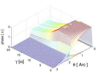
Figure 1: An illustration of the geometric phases of the two-level system coupling to the environment at time $T=2\pi/\omega.$

The open system effect in geometric phase may be observed with a combination of the engineering reservoir technique myatt00 and the Mach-Zehnder atom interferometer featonby98 ; webb99 , in which each of the arms consists of an atom in a dark state. The dark state can be realized in the atom-light system that consists of cesium atoms interacting with light resonant with the $F=3\rightarrow F^{{}^{\prime}}=3$ transitions of the $D1\ \ 6^{2}s_{1/2}\rightarrow 6^{2}p_{1/2}$ line. It makes the dynamical phase negligible with respect to the geometric phase. A dephasing engineering reservoir in one arm of the interferometer, which may be simulated by variations of the light fields, would give a relative phase to the atom passing though the arm, the output interference pattern yields the geometric phase of the atom system.

One of the key assumptions of our representation is the dephasing condition, i.e., $[H_{S},H_{I}]=0$. Using ground states as the qubits can make the formulation exact. Suppose now there is an small additional term in $H_{I}$, $H_{I}^{{}^{\prime}}=\sum_{m}Y_{m}(\Gamma_{m}+\Gamma_{m}^{\dagger})$, that breaks the dephasing condition. Simple algebra shows that the transition probability between $|E_{m}\rangle$ and $|E_{n}\rangle$ due to coupling $Y_{p}(\Gamma_{p}+\Gamma_{p}^{\dagger})$ is proportional to $|\gamma_{p}\langle E_{n}|Y_{p}|E_{m}\rangle|^{2}/|E_{m}-E_{n}|^{2}$, where $\gamma_{p}$ denotes the maximum of average values of $(\Gamma_{p}+\Gamma_{p}^{\dagger})$. In the case of $|\gamma_{p}\langle E_{n}|Y_{p}|E_{m}\rangle|<<|E_{m}-E_{n}|$, the open system may be treated as a dephasing system, because the transition between any different eigenstates of the system may be ignored. The case where this transition could not be ignored will be discussed in the next section.

IV geometric phase in dissipative systems: exactly solvable model

In this section, we will consider a spin-$\frac{1}{2}$ particle interacting with an environment formed by $N$ independent spins through the Hamiltonian

$$H=\Delta\sigma_{x}+\frac{1}{2}\sum_{k=1}^{N}g_{k}\sigma_{z}\sigma_{z}^{(k)},$$ (15)

where $\sigma_{i}^{(k)}$ and $\sigma_{i}$, $i=x,y,z$ denote Pauli operators for the environment and spin-$\frac{1}{2}$ particle, respectively. $g_{k},(k=1,2,...,N)$ are coupling constants, term with $\Delta$ stands for the self-Hamiltonian of the particle. This model is interesting because the pointer states do not coincide with the eigenstates of the interaction Hamiltonian, but can range from coherent sates to eigenstates of the system’s Hamiltonian determining by the interplay between the self-Hamiltonian and the interaction with the environment. We will calculate the geometric phase gained by the particle beyond the Markov approximation and the weak coupling limit. The dynamics govern by Hamiltonian Eq.(15) can be solved exactly by a standard procedurecucchietti05 , it yields the reduced density matrix of the particle as

$$\rho(t)=(I+\vec{p}(t)\cdot\vec{\sigma})/2,$$ (16)

where $\vec{p}(t)$ is the polarization vector given by $\vec{p}(t)=\int\vec{p}(t,B)\eta(B)dB$ with $\Omega_{B}^{2}=\Delta^{2}+B^{2}$ and

$$\eta(B) = \frac{1}{\sqrt{2\pi s_{N}^{2}}}e^{-B^{2}/2s_{N}^{2}},$$

$$p_{x}(t,B) = p_{x}(0)\frac{\Delta^{2}+B^{2}\cos(2\Omega_{B}t)}{\Omega_{B}^{2}}-p_{y}(0)\frac{B}{\Omega_{B}}\sin(2\Omega_{B}t)$$

$$+ p_{z}(0)\frac{2\Delta B}{\Omega_{B}^{2}}\sin^{2}(\Omega_{B}t),$$

$$p_{y}(t,B) = p_{y}(0)\cos(2\Omega_{B}t)+\frac{\sin(2\Omega_{B}t)}{\Omega_{B}}\left[p_{x}(0)B-\Delta p_{z}(0)\right],$$

$$p_{z}(t,B) = p_{z}(0)\frac{B^{2}+\Delta^{2}\cos(2\Omega_{B}t)}{\Omega_{B}^{2}}$$ (17)

$$+ p_{x}(0)\frac{2\Delta B}{\Omega_{B}^{2}}\sin^{2}(\Omega_{B}t)+p_{y}(0)\frac{\Delta}{\Omega_{B}}\sin(2\Omega_{B}t).$$

To get this result, it is only required that the couplings $g_{k}$ of Eq.(15) are sufficiently concentrated near their average value so that their standard deviation exists and is finite.

By rewriting the reduced density matrix $\rho(t)$ in the form

$$\rho(t)=\lambda_{1}(t)|\psi_{1}(t)\rangle\langle\psi_{1}(t)|+\lambda_{2}(t)|\psi_{2}(t)\rangle\langle\psi_{2}(t)|,$$ (18)

we get the geometric phasetong04 of the particle acquired at time $\tau$,

$$\Phi_{g}^{\prime}(\tau)=arg\left(\sum_{i=1,2}\sqrt{\lambda_{i}(0)\lambda_{i}(\tau)}\langle\psi_{i}(0)|\psi_{i}(\tau)\rangle e^{-\int_{0}^{\tau}\langle\psi_{i}(t)|\frac{\partial}{\partial t}|\psi_{i}(t)\rangle dt}\right).$$ (19)

After simple manipulations, we arrive at

$$\Phi_{g}^{\prime} = arg[\Lambda_{1}(\tau)(\cos\frac{\theta(0)}{2}\cos\frac{\theta(\tau)}{2}e^{-i(\phi(\tau)-\phi(0))}$$ (20)

$$+ \sin\frac{\theta(0)}{2}\sin\frac{\theta(\tau)}{2})e^{iC}$$

$$+ \Lambda_{2}(\tau)(\cos\frac{\theta(0)}{2}\cos\frac{\theta(\tau)}{2}e^{i(\phi(\tau)-\phi(0))}$$

$$+ \sin\frac{\theta(0)}{2}\sin\frac{\theta(\tau)}{2})e^{-iC}].$$

Here,

$$\Lambda_{1,2}=\frac{1}{2}\sqrt{(1\pm|\vec{p}(0)|)(1\pm|\vec{p}(t)|)},$$

$$\cos\theta(t)=\frac{p_{z}(t)}{\sqrt{p_{x}^{2}(t)+p_{y}^{2}(t)+p_{z}^{2}(t)}},$$

$$\tan\phi(t)=\frac{p_{y}(t)}{p_{x}(t)},$$

$$C=\frac{i}{2}\left(\int_{0}^{\tau}\frac{\partial\phi}{\partial t}dt+\int_{0}^{\tau}\cos\theta\frac{\partial\phi}{\partial t}dt\right).$$

The dependence of the geometric phase $\Phi_{g}^{\prime}$ on the variance $s_{N}$ and system free energy $\Delta$ is complicated, we discuss here on two limiting cases $s_{N}\gg\Delta$ and $s_{N}\ll\Delta$ with a specific initial state $p_{x}(0)=1,p_{y}(0)=p_{z}(0)=0$. In $s_{N}\gg\Delta$ limit, the dynamics of the spin-$\frac{1}{2}$ particle is so slow that its behavior should approach $p_{x}(t)=e^{-2t^{2}s_{N}^{2}}$ and $p_{y}(t)=p_{z}(t)=0,$ which yields $\Phi_{g}^{\prime}=0$ because $\phi=0$ in this limit with the initial state. In $s_{N}\ll\Delta$ limit, Eq.(17) follows that,

$$p_{x}(t) \simeq p_{x}(0)\left[\gamma\left(\frac{\Delta}{\sqrt{2}s_{N}}\right)+\frac{\cos\left(2\Delta t+\frac{3\pi}{4}\right)}{\sqrt{8\Delta s_{N}^{2}t^{3}}}\right],$$

$$p_{y}(t) = p_{z}(t)=0,$$ (21)

where $\gamma(x)=\sqrt{\pi}xe^{x^{2}}\left(1-{\rm Erf}(x)\right),$ $Erf(x)$ is the error function, and $\gamma\left(\frac{\Delta}{\sqrt{2}s_{N}}\right)\ll 1$ in this limit. By Eq.(20), it is clear that $\Phi_{g}^{\prime}=0$ in this limit, too. The numerical result for the geometric phase as a function of $\Delta$ and $s_{N}$ was shown in figure 2. To plot this figure, we assume that the system has evolved for time $\tau=2\pi/\Delta$, which is the characterized time for the system undergoing a free evolution. Figure 2 shows that the geometric phase is zero in the two limiting cases $\Delta\gg s_{N}$ and $\Delta\ll s_{N}$ as expected. There are sharp changes among the line $\Delta\sim s_{N}$, indicating a crossover from the limit $\Delta\ll s_{N}$ to $\Delta\gg s_{N}.$

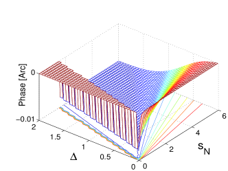
Figure 2: The geometric phase of the spin-$\frac{1}{2}$ particle versus $s_{N}$ and $\Delta$. The spin was dissipatively coupled to an environment and the phase was calculated at time $\tau=2\pi/\Delta$, depending on the time scale of free evolution of the particle.

V summary and discussion

We have presented a general calculation the geometric phase in open systems subject to dephasing and dissipation, the calculations are beyond the quantum Markov approximation and the weak coupling limit. For the dephasing system, it acquires no geometric phase with the decoherence rate $\gamma\rightarrow\infty$, this can be explained as an effect of decoherence on the geometric phase, i.e., the quantum system could not maintain its phase information after the decoherence time. There is a sharp change along the line $\theta=\pi/2$ as figure 1 shown, this can be understood in terms of the Bloch sphere that represents the state of the system. The geometric phase increases due to decoherence when initial states fall onto the upper semi-sphere, but it decrease when the initial states on the lower semi-sphere. These results are similar to the prediction given by the quantum trajectory analysis for dissipative systems. The geometric phase $\Phi_{g}^{\prime}$ in dissipative systems is always zero as long as $p_{x}(t)/p_{y}(t)=$constant, this is exactly the case when $\Delta/s_{N}\rightarrow\infty$ or $\Delta/s_{N}\rightarrow 0$. $\Delta/s_{N}\rightarrow\infty$ implies that the self energy $\Delta$ of the particle is much larger than the cumulative variance $s_{N}$ of the coupling constants $g_{k}$. For $g_{k}$ taking the value $+g$ or $-g$ ($g$ arbitrary) with equal probability, $s_{N}^{2}=\sum_{k}g_{k}^{2}.$ This tells us that the geometric phase is zero when the self-Hamiltonian dominates. On the other hand, when $\Delta/s_{N}\rightarrow 0$ the interaction Hamiltonian dominates, pointer states in this situation coincide with the eigenstates of the interaction Hamiltonian, thus the spin-$\frac{1}{2}$ particle could not acquire geometric phase. In the crossover regime $\Delta\sim s_{N}$, the geometric phase change sharply due to the interplay between the self-Hamiltonian and the interaction with the environment.

These results constitute the basis of a framework to analyze errors in the holonomic quantum computation, where two kinds of errors are believed to affect its performance. This first error would take the system out of the degenerate computation subspace, while the second takes place within the subspace. The first kind of error can be eliminated by working in the ground states and having a system where the energy gap with the first excited state is very large. The second kind of error falls to the regime analyzed in Sec. II and III, since there is no dissipation but dephasing in the system, while the first belongs to the regime discussed in Sec. IV. The calculation presented here in principle allows one to study the geometric phase at any timescale, and hence it has advantages with respect to any treatment with approximations in most literatures.

X.X.Y. acknowledges simulating discussions with Dr. Robert Whitney. This work was supported by EYTP of M.O.E, NSF of China (10305002 and 60578014), and the NUS Research Grant No. R-144-000-071-305.

References

- (1) M. V. Berry, Proc. R. Soc. London A 392, 45(1984).
- (2) Geometric phase in physics, Edited by A. Shapere and F. Wilczek ( World Scientific, Singapore, 1989).
- (3) A. Uhlmann, Rep. Math. Phys. 24, 229 (1986).
- (4) E. Sjöqvist, A.K. Pati, A. Ekert, J.S. Anandan, M. Ericsson, D.K.L. Oi, and V. Vedral, Phys. Rev. Lett. 85, 2845 (2000).
- (5) I. Fuentes-Guridi, A. Carollo, S. Bose, and V. Vedral, Phys. Rev. Lett. 89, 220404 (2002); A. Carollo, I. Fuentes-Guridi, M. Franca Santos and V. Vedral, Phys. Rev. A 67, 063804(2003).
- (6) X.X. Yi, L.C. Wang, and T.Y. Zheng, Phys. Rev. Lett. 92, 150406 (2004); X. X. Yi, and E. Sjöqvist, Phys. Rev. A 70, 042104 (2004); L. C. Wang, H. T. Cui, and X. X. Yi, Phys. Rev. A 70, 052106 (2004).
- (7) P. Zanardi and M. Rasetti, Phys. Lett. A 264, 94 (1999).
- (8) J. A. Jones, V. Vedral, A. Ekert, and G. Castagnoli, Nature (London) 403, 869 (1999).
- (9) A. Ekert, M. Ericsson, P. Hayden, H. Inamori, J.A. Jones, D.K.L. Oi, and V. Vedral, J. Mod. Opt. 47, 2051 (2000).
- (10) G.Falci, R. Fazio, G.M. Palma, J. Siewert, and V. Vedral, Nature (London) 407, 355 (2000).
- (11) J. C. Garrison and E. M. Wright, Phys. Lett. A 128, 177(1988).
- (12) K. M. Fonseca Romero, A. C. Aguira Pinto, and M. T. Thomaz, Physica A 307, 142(2002).
- (13) A. C. Aguira Pinto and M. T. Thomaz, J. Phys. A: Math. Gen. 36, 7461(2003).
- (14) D. Ellinas, S. M. Barnett, and M. A. Dupertuis, Phys. Rev. A 39, 3228(1989).
- (15) D. Gamliel and J. H. Freed, Phys. Rev. A 39, 3238(1989).
- (16) I. Kamleitner, J. D. Cresser, and B. C. Sanders, Phys. Rev. A 70, 044103(2004).
- (17) A. Nazir, T. P. Spiller, W. J. Munro, Phys. Rev. A 65, 042303(2002).
- (18) A. Carollo, I. Fuentes-Guridi, M. Franca Santos, and V. Vedral, Phys. Rev. Lett. 90,160402(2003); ibid 92, 020402(2004).
- (19) K. P. Marzlin, S. Ghose, and B. C. Sanders, Phys. Rev. Lett. 93, 260402 (2004).
- (20) R. S. Whitney, and Y. Gefen, Phys. Rev. Lett. 90, 190402(2003); R. S. Whitney, Y. Makhlin, A. Shnirman, and Y. Gefen, e-print:cond-mat/0405267.
- (21) F. Gaitan, Phys. Rev. A 58, 1665(1998).
- (22) X. X. Yi, L. C. Wang, and W. Wang, Phys. Rev. A 71, 044101 (2005).
- (23) D. M. Tong, E. Sjöqvist, L. C. Kwek, C. H. Oh, Phys. Rev. Lett. 93, 080405 (2004).
- (24) C. P. Sun, X. X. Yi, X. J. Liu, Fortschritte Der Physik 43, 585 (1995).
- (25) was assumed nondegenerate, for the degenerate case, we may choose some linear combination of the degenerate eigenstates as the new eigenstates of , such that are also belong to .
- (26) I. Fuentes-Guride, F. Girelli, and E. Livine, Phys. Rev. Lett. 94, 020503(2005).
- (27) C. J. Myatt, B. E. King, Q. A. Turchette, C. A. Sackett, D. Kielpinski, W. M. Itano, C. Monore, and D. J. Wineland, Nature(London) 403, 269(2000).
- (28) P. D. Featonby et al., Phys. Rev. Lett. 81, 495(1998).
- (29) C. L. Webb et al., Phys. Rev. A 60, R1783 (1999).
- (30) F. M. Cucchietti, J. P. Paz, and W. H. Zurek, Phys. Rev. A 72, 052113(2005).