Randomized Dynamical Decoupling Techniques for Coherent Quantum Control

Abstract

The need for strategies able to accurately manipulate quantum dynamics is ubiquitous in quantum control and quantum information processing. We investigate two scenarios where randomized dynamical decoupling techniques become more advantageous with respect to standard deterministic methods in switching off unwanted dynamical evolution in a closed quantum system: when dealing with decoupling cycles which involve a large number of control actions and/or when seeking long-time quantum information storage. Highly effective hybrid decoupling schemes, which combine deterministic and stochastic features are discussed, as well as the benefits of sequentially implementing a concatenated method, applied at short times, followed by a hybrid protocol, employed at longer times. A quantum register consisting of a chain of spin-1/2 particles interacting via the Heisenberg interaction is used as a model for the analysis throughout.

I Introduction

The constructive role of randomness in physical processes has been demonstrated in various areas of research. In stochastic resonance Gammaitoni , for instance, a weak signal can be amplified by the assistance of an appropriate noise. In quantum information processing, noise can intensify the speed-up of quantum walks over classical ones Kendon , dissipation may offer new possibilities to implement gate operations in quantum computing Beige , while static perturbations characterizing faulty gates can enhance the stability of quantum algorithms Prosen . In quantum communication, the use of random operations decreases the communication cost of achieving remote state preparation and of constructing efficient quantum data-hiding schemes Hayden . Finally, random unitary operators have been recently suggested as allowing efficient parameter estimation for open quantum systems EmersonSc .

In the context of coherent quantum control, the advantages of stochasticity have only recently been addressed Viola2005Random ; Kern2004 ; Kern2005 ; Santos2005 ; Kern2006 ; Santos2006 . Within the framework of dynamical decoupling methods, in particular, analytical bounds derived in Viola2005Random pointed to situations where randomized protocols are expected to outperform their deterministic counterparts in suppressing unwanted unitary dynamics as well as decoherence in open quantum systems. The idea of merging together deterministic and randomized designs into hybrid control schemes, where benefits from both approaches may be simultaneously exploited, was also proposed in Viola2005Random in general control-theoretic terms, and independently validated in illustrative situations in Kern2005 ; Santos2005 ; Kern2006 (see also Santos2006 ).

Here, we focus on exploring the advantages of randomization in establishing efficient control schemes for arbitrary quantum state stabilization, that is, for engineering a quantum memory. Efficiency is assessed in terms of both the number of control operations needed to achieve a desired fidelity level and the rate at which residual errors build up in the long run. We show that by interpolating the most effective (deterministic) scheme known for short-time decoupling with the best available (randomized) scheme for long time, very high performance over the entire time axis may be ensured.

II System and Control Setting

Dynamical decoupling (DD) techniques have been extensively discussed both in the original high-resolution nuclear magnetic resonance (NMR) setting Haeberlen and, more recently, in connection with robust quantum information processing, see for instance Viola98 ; Viola1 ; DDqubits for representative contributions. Assume, for simplicity, an isolated finite dimensional target system ${\cal S}$ described by a (possibly) time dependent Hamiltonian $H_{0}(t)$. The basic idea of DD is to modify the dynamics of ${\cal S}$ by adding to $H_{0}(t)$ an appropriate time-dependent control field $H_{c}(t)$. The overall propagator under the total Hamiltonian and the control propagator in units $\hbar=1$ are, respectively, $U(t)={\cal T}\exp[-i\int_{0}^{t}(H_{0}(u)+H_{c}(u))du]$ and $U_{c}(t)={\cal T}\exp[-i\int_{0}^{t}H_{c}(u)du]$, where ${\cal T}$ indicates time ordering. A transformation to a logical frame that removes $H_{c}(t)$ is commonly performed, leading to a controlled evolution described by

$$\tilde{U}(t)=U_{c}^{\dagger}(t)U(t)={\cal T}\exp\left[-i\int_{0}^{t}{\tilde{H}_{0}}(u)du\right]\>,$$ (1)

where ${\tilde{H}_{0}}(t)=U^{\dagger}_{c}(t)H_{0}(t)U_{c}(t)$ is the logical Hamiltonian. When $H_{0}(t)$ is time-independent and the perturbation is cyclic with cycle time $T_{c}$, i.e. $U_{c}(T_{c})={\mathbb{1}}$, where ${\mathbb{1}}$ is the identity operator, physical and logical frame coincide stroboscopically at $T_{n}=nT_{c}$, $n\in{\mathbb{N}}$. Using the formalism of average Hamiltonian theory (AHT), the evolution operator in the logical frame may be expressed as $\tilde{U}(nT_{c})=\exp(-i{\bar{H}_{0}}nT_{c})$, where

$$\tilde{U}(T_{c})={\cal T}\exp\left[-i\int_{0}^{T_{c}}{\tilde{H}_{0}}(u)du\right]\equiv e^{-i{\bar{H}}_{0}T_{c}}$$ (2)

defines the average Hamiltonian ${\bar{H}_{0}}=\sum_{k=0}^{\infty}{\bar{H}_{0}}^{(k)}$, with each term ${\bar{H}_{0}}^{(k)}$ computed from the Magnus expansion ErnstBook ; HaeberlenBook . A sufficient convergence criterion for the series is given by $\kappa T_{c}<1$, where $\kappa=||H_{0}||_{2}$ and $||A||_{2}=\max|{\rm eig}(A)|$, $\forall A=A^{\dagger}$.

The above time average for ${\bar{H}_{0}}$ may be conveniently mapped into a group-theoretic average. In the framework of bang-bang DD, in particular, control actions correspond to arbitrarily strong and effectively instantaneous rotations successively drawn from a (projective representation of a) group, ${\cal G}=\{g_{j}\}$, $j=0,\ldots,|{\cal G}|-1$. The propagator at $T_{c}$ is written as

$$\tilde{U}(T_{c})=U(T_{c})=\prod_{k=0}^{|{\cal G}|-1}g_{k}^{\dagger}U_{0}(t_{k+1},t_{k})g_{k}\>,$$ (3)

which translates into a cyclic sequence of pulses $P_{k}=g_{k}g_{k-1}^{\dagger}$, $k=1,\ldots,|{\cal G}|$, separated by intervals $\Delta t=t_{k+1}-t_{k}$ of free evolutions, leading in turn to a cycle time $T_{c}=|{\cal G}|\Delta t$. The zeroth order contribution of the Magnus expansion, which dominates in the limit $T_{c}\rightarrow 0$, is therefore ${\bar{H}_{0}}^{(0)}=\bar{H}_{\cal G}={|{\cal G}|^{-1}}\sum_{j}{g_{j}^{\dagger}H_{0}g_{j}}$.

The so-called time suspension is the DD goal we focus on here, that is, we want to develop pulse sequences able to approximate the evolution operator as close as possible to $\mathbb{1}$. How well we succeed at preserving a given initial state $|\psi\rangle$ is reflected, for instance, in the proximity of the input-output fidelity $F(T)$ to its maximum value 1, where $F_{|\psi\rangle}(T)=|\langle\psi|U(T)|\psi\rangle|^{2}$.

A deterministic protocol based on a fixed control path of a representation of ${\cal G}$ and aiming at achieving first-order decoupling, ${\bar{H}_{0}}^{(0)}=0$, will be referred to as “periodic deterministic decoupling” (PDD) protocol remark . We will assume here that the first PDD pulse occurs only at $t_{1}=\Delta t$, that is, $g_{0}=\mathbb{1}$. Its simplest stochastic version is obtained by randomly picking elements over ${\cal G}$, such that the control action at each $t_{n}=n\Delta t$ [$t_{0}$ included] corresponds to $P^{(r)}=g_{i}g_{j}^{\dagger}$, $i,j=0,\ldots,|{\cal G}|-1$. This leads to what we call “naïve random decoupling” (NRD) – an intrinsically acyclic method. Bounds on the worst-case pure-state expected fidelity at time $T$, $F(T)={\rm min}_{|\psi\rangle}F_{|\psi\rangle}(T)$, were established in Ref. Viola2005Random . For PDD, in the limit $TT_{c}\kappa^{2}\ll 1$, we have: $F(T)\geq 1-{\cal O}(T^{2}T_{c}^{2}\kappa^{4})$, while for NRD and $T\Delta t\kappa^{2}<1$: ${\mathbb{E}}\{F(T)\}\geq 1-{\cal O}(T\Delta t\kappa^{2})$, where ${\mathbb{E}}$ denotes ensemble expectation over all control realizations. We note that the bound for NRD still holds in the case of a time dependent Hamiltonian as far as $||H_{0}(t)||_{2}$ is uniformly bounded in time by $\kappa>0$. Within their regime of validity, these bounds indicate that NRD should outperform PDD when $|{\cal G}|^{2}(T\Delta t\kappa^{2})\gg 1$, which is the case when large control groups and/or long interaction times are involved.

In practice, we avoid the extremization procedure required to determine the worst-case pure-state expected fidelity. Instead, in order to get a state-independent estimate of the performance of different DD methods, we invoke gate entanglement fidelity, $F_{e}(T)$ Schumacher . This quantity is linearly related to the average input-output fidelity over all pure states of the system Nielsen ; Fortunato , and it may be computed as $F_{e}(T)=|\mbox{Trace}(U(T))/d|^{2}$, where $d$ is the dimension of the system’s state space. Our control objective is then to get as close as possible to ${\mathbb{E}}\{F_{e}(T)\}\rightarrow 1$. In the Monte Carlo simulations to be presented below, ensemble expectation, ${\mathbb{E}}\{F_{e}(T)\}$, is further replaced by an average over a sufficiently large statistical sample of control realizations, leading to what we denote $\langle\langle F_{e}\rangle\rangle$.

In order to concretely illustrate the benefits of randomization, we concentrate on a relatively simple, yet physically relevant, example – that is, to completely refocus the internal evolution of a chain consisting of $N$ strongly coupled spin-1/2 particles (qubits) described by the Heisenberg model,

$$H_{0}=\sum_{i=1}^{N}\frac{\omega_{i}Z_{i}}{2}+J\sum_{i=1}^{N-1}\left(X_{i}X_{i+1}+Y_{i}Y_{i+1}+\Delta Z_{i}Z_{i+1}\right)\>.$$ (4)

Here $X,Y$, and $Z$ denote Pauli operators, $\omega_{i}$ is the frequency of qubit $i$, $J$ is the coupling parameter, and $\Delta$ determines the anisotropy. Only nearest-neighbor interactions are considered, which is a fairly good approximation for couplings exponentially decaying with the qubit distance – as arising, for instance, in quantum dot arrays Loss – or decaying cubically – as it is the case for dipolar interactions of NMR crystals and liquid-crystals HaeberlenBook ; Baugh2005 , or electrons on Helium Dykman01 .

We consider qubits with approximately the same frequency $\omega_{i}\approx\omega$. Accordingly, in order to remove the phase evolution due to the one-body Zeeman terms, we perform a transformation to a frame rotating with frequency $\omega$ and characterized by the operator $U_{R}(t)=\exp[-i\omega t\sum_{i}^{N}Z_{i}/2]$. We thus work in a combined logical-rotating frame, whereby the effective Hamiltonian becomes ${\tilde{H}}_{R}(t)=U^{\dagger}_{c}(t)U^{\dagger}_{R}(t)[H_{0}(t)-\omega\sum_{i}Z_{i}/2]U_{R}(t)U_{c}(t)$. While this approximation is accurate for a class of physical systems (notably, homonuclear NMR samples), the restriction is not fundamental. If the spread of the single-qubit is significant (so that a common rotating frame does not exist), schemes capable of additionally refocusing the Zeeman terms may be constructed without adding to the overall complexity of the DD procedure Stoll .

III Convergence Improvement

Following the general idea of Stoll ; Viola1 , a PDD protocol capable of refocusing the nearest-neighbor couplings of Eq. (4) for arbitrary parameter values may be built by recursively nesting DD sequences based on the group ${\cal G}_{i}=\{{\mathbb{1}}_{i},Z_{i},X_{i},Y_{i}\}$ for each even qubit, $i=2,4,\ldots,2m$, where $N=2m$ or $N=2m+1$, $m\in{\mathbb{N}}$. For instance, when $N=4$ or 5, a possible DD scheme may be visualized in terms of the following matrix,

$$M=\left(\begin{array}[]{cccccccccccccccc}\mathbb{1}&Z&X&Y&Y&X&Z&\mathbb{1}&\mathbb{1}&Z&X&Y&Y&X&Z&\mathbb{1}\\ \mathbb{1}&\mathbb{1}&\mathbb{1}&\mathbb{1}&Z&Z&Z&Z&Y&Y&Y&Y&X&X&X&X\par\end{array}\right),$$

where each row corresponds to an even qubit and each column, supplemented with the identity operators associated to the odd qubits, leads to an element of the DD group, so that ${\cal G}=\{g_{j}\}$, $j=0,\ldots,|{\cal G}|-1$ and $g_{j}=\mathbb{1}_{1}\otimes[M_{(1,j+1)}]_{2}\otimes\mathbb{1}_{3}\otimes[M_{(2,j+1)}]_{4}\otimes\mathbb{1}_{5}$. Although this scheme does not scale efficiently, as the number of $\pi$ pulses required to close a cycle grows as $4^{m}$, it allows for the study of the effects of large control groups in DD methods with no need to employ excessively large systems. Numerical simulations with moderate computational resources become then viable. Contrary to PDD, where only one qubit is rotated at a time, the NRD sequence associated to the above ${\cal G}$ involves random pulses ranging from the identity operator to $m$ simultaneous rotations. The total number of random pulses leading to $R$ simultaneous rotations is given by $Q_{R}=3^{R}m!/[R!(m-R)!]$, where $\sum_{R=0}^{m}Q_{R}=4^{m}$. In large systems, the percentage of random pulses corresponding to a single qubit rotation, or at the other extreme, to $R=m$, is very small, decreasing with the size of the system, respectively, as $3m/4^{m}$ and $(3/4)^{m}$. When $m\neq 3+4n$, the largest $Q_{R}$ is obtained for the integer $R$ in the interval $[(3m-1)/4,(3m+3)/4]$, while for $m=3+4n$, both values $R=(3m-1)/4$ and $R=(3m+3)/4$ lead to the two largest subsets of random pulses.

In Fig. 1, $N=8$ qubits are considered, leading to a relatively large control cycle: 256 time slots. Two situations favoring stochastic schemes are identified. On the left panel, the average fidelity is computed at every $T_{n}=n|{\cal G}|\Delta t$. Even though PDD achieves first-order decoupling at these instants, the fidelity decay is substantially slower for NRD. This behavior persists even when the $\Delta t$ value of PDD is shorter than that of NRD. Irrespective of the validity of the strict short-time condition underlying the bounds of Viola2005Random , these findings confirm the faster convergence offered by stochastic methods when $|{\cal G}|$ is large. The fact that NRD eventually surpasses both PDD curves shows that, for sufficiently long times, the constraints on $\Delta t$ for random DD may be relaxed or, equivalently, the number of control operations able to ensure a certain fidelity level may be smaller than in PDD. Both features may be very advantageous in realistic settings, given that achievable pulsing rates are finite and excessive ‘kicks’ might be undesirable (leading e.g. to unwanted heating in devices operating at dilution-refrigerator temperatures, such as quantum dots). Similar improvements are observed in situations where constraints on the number of pulses or control intervals make it unfeasible to close a complete cycle. This may be the case, for instance, when $T_{c}$ becomes prohibitively long. Here, no analytical fidelity bound for PDD exists, hence we rely exclusively on numerical simulations. When compared with the particular PDD sequence considered, NRD performs significantly better for most intra-cycle times $t_{n}=n\Delta t<T_{c}$, a result that prompts the search for superior deterministic sequences. Designing new stochastic methods capable of pre-filtering potentially good sequences simplifies this search, which would otherwise be performed over the extremely large ensemble, size of ${\cal O}(|{\cal G}|^{n|{\cal G}|})$, generated by NRD. More efficient randomized protocols will be discussed in the next section.

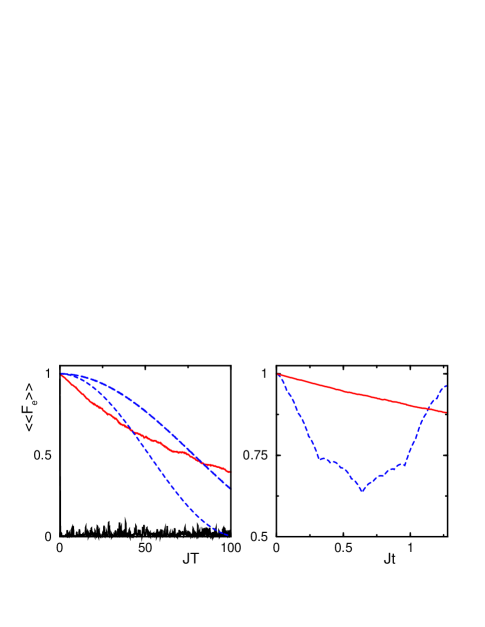
Figure 1: (color online) PDD vs. NRD based on a nested pulse sequence for Hamiltonian (4) with $\Delta=1$ and $N=8$ in the logical-rotating frame. Left panel: average fidelity at $T_{n}=n|{\cal G}|\Delta t$, $|{\cal G}|=4^{4}$. PDD: $T_{c}=0.08J^{-1}$ - (blue) dashed line, $T_{c}=0.12J^{-1}$ - (blue) short-dashed line; NRD: (red) solid line, $\Delta t=0.12J^{-1}/4^{4}$, average over $50$ realizations. Free evolution: (black) oscillating solid line. Right panel: average fidelity within a cycle, $t_{n}=n\Delta t$ with $\Delta t=0.005J^{-1}$ for both protocols, average over $10^{2}$ realizations.

IV Long-time Improvement

Conceptually, there are two main strategies for boosting DD performance. One rests on ways for increasing the averaging accuracy (hence the minimum power of $\Delta t$) in the effective Hamiltonian, the other on slowing down the accumulation of residual errors due to imperfect averaging over long times. Based on these guiding principles, we introduce several DD schemes and discuss their relative merits.

In the deterministic domain, one possibility is motivated by the Carr-Purcell sequence of NMR, and consists of symmetrizing in time the control path of the PDD. It leads to what we call “symmetric deterministic DD” (SDD). The cycle becomes twice as long, but all odd order terms in ${\bar{H}_{0}}$ are also canceled. Another scheme, which generalizes NMR supercycle techniques HaeberlenBook , corresponds to “concatenated DD” (CDD), as recently formalized in Khodjasteh2004 . CDD has a temporal recursive structure, whose level $\ell+1$ of concatenation is determined by the pulse sequence $C_{\ell+1}=C_{\ell}P_{1}C_{\ell}P_{2}\ldots C_{\ell}P_{N}$, where $P_{k}$ is the $k$th pulse, $C_{0}$ is the inter-pulse interval and $C_{1}$ denotes the generating PDD sequence. At level $\ell=2$ the concatenated sequence is also symmetric. Interestingly, however, CDD may outperform SDD even before this level of concatenation is actually completed, reflecting its superiority in reducing the accumulation of errors.

In terms of randomized DD, we introduce hybrid protocols, which combine deterministic and stochastic features. The purpose here is to ensure good performance at short times, as typical of deterministic protocols, while at long times, instead of accumulating errors coherently, randomization guarantees this to happen probabilistically. The protocols are classified according to an inner and an outer code. The former establishes the pulse sequence in the interval $[n|{\cal G}|\Delta t,(n+1)|{\cal G}|\Delta t]$, being associated with the control path chosen to traverse ${\cal G}$. Since the group is traversed in full, as in deterministic schemes, the inner code leads to an effective Hamiltonian $H_{\rm eff}\propto{\cal O}(\Delta t)$. The outer code determines the additional random pulses to be applied at $T_{n}=n|{\cal G}|\Delta t$. The latter are drawn from a group ${\cal G}^{\prime}$, which needs not coincide with ${\cal G}$. Randomization may then be associated with the choice for the inner code or the outer code. In the first category we have the “random path decoupling” (RPD) protocol, as proposed in Viola2005Random . It consists of randomly choosing, at every $T_{n}$, which control path to follow to traverse ${\cal G}$. Here, as in most stochastic protocols, logical and physical frame do not always coincide and we need to keep track of the applied control trajectory, so that an appropriate control operation may be used to correct frames. However, similarly to PDD, we may choose to fix the first group element as ${\mathbb{1}}$, which leads to frame coincidenece at every $T_{n}$. This may be particularly useful, for instance, in conventional line-narrowing spectroscopic applications. We will call this alternative “pseudo-random path decoupling” (pRPD). To the second category belongs the embedded scheme (EMD), inspired to Kern2005 . The inner code is a fixed PDD sequence, while the bordering pulses may either be picked at random from ${\cal G}$ or from a different control set, corresponding, for example to products of uncorrelated Pauli operators as described in Kern2005 . Contrary to RPD, this protocol may suffer from non-uniform performance across the set of $|{\cal G}|!$ possible inner paths, requiring a pre-selection of a good deterministic pulse sequence. The performance of both EMD and RPD is significantly improved by further symmetrizing the inner control path in the same manner as in SDD. Here, we will be dealing only with the “symmetric random path decoupling” (SRPD) protocol.

IV.1 Bounds on Fidelity Decay

Analytical upper bounds on the order of the fidelity decay, $1-{\mathbb{E}}\{F_{e}(T)\}$, may give an insight on what to expect from the above protocols. Generalizing the arguments of Viola2005Random ; Kern2005 , we find the following order-of-magnitude estimates for deterministic (top line) and stochastic (bottom line) schemes:

PDD	SDD
$T^{2}(|{\cal G}|\Delta t)^{2}\kappa^{4}$	$T^{2}(|{\cal G}|\Delta t)^{4}\kappa^{6}$

NRD	RPD/EMD	SRPD
$T\Delta t\kappa^{2}$	$T(|{\cal G}|\Delta t)^{3}\kappa^{4}$	$T(|{\cal G}|\Delta t)^{5}\kappa^{6}$

For deterministic protocols, residual errors add coherently, which leads to a quadratic-in-time fidelity decay, ${\cal O}((T||{\bar{H}_{0}}||_{2})^{2})$, as found in Viola2005Random . Therefore, it is only the ability to cancel or reduce higher order terms in ${\bar{H}_{0}}$ that may induce better performance. At short times, the dominant term in each cycle of the PDD is ${\bar{H}_{0}^{(1)}}$, and the bound is derived from the norm $||{\bar{H}_{0}^{(1)}}||_{2}\leq\kappa^{2}T_{c}$. For SDD, ${\bar{H}_{0}^{(1)}}=0$, and the norm of the dominant term is limited as $||{\bar{H}_{0}^{(2)}}||_{2}\leq\kappa^{3}T_{c}^{2}$. In the case of CDD, the averaging accuracy depends on the level of concatenation (level 1 recovering the results of PDD) and on the system considered.

Contrasted with deterministic methods, the accumulation of residual errors for random protocols is slower, as reflected by the linear-in-time decay of the fidelity. This may be intuitively justified as follows. Each step of NRD can accumulate an error amplitude up to $\kappa\Delta t$ and during a time $T$ there are $T/\Delta t$ such intervals. Due to the randomization, amplitudes add up probabilistically, leading to a decay $\propto T\Delta t\kappa^{2}$. The reasoning is similar for the other protocols, but each step now corresponds to the total interval of the inner code, $p|{\cal G}|\Delta t$, $p=1$ [$p=2$] for RPD/EMD [SRPD], leading to ${\mathbb{E}}\{F_{e}(T)\}\geq 1-{\cal O}(T|{\cal G}|\Delta t||{\bar{H}_{\rm eff}}||_{2}^{2})$. The norm of the effective Hamiltonian is derived from the deterministic sequence underlying the stochastic protocol, the worst path being considered for RPD/SRPD. Hence $||{\bar{H}_{\rm eff}}||_{2}\sim||{\bar{H}_{0}}||_{2}$ and here again $||{\bar{H}_{0}}||_{2}$ becomes the main factor differentiating the protocols. We therefore expect a significant better performance for SRPD (whose norm comes from SDD) than for RPD/EMD (whose norm is that of PDD).

Merging together features of deterministic methods and pulse randomization, as in hybrid DD schemes, suggests the possibility of suppressing errors more effectively at both short and long interaction times. However, since the above bounds apply only at short times, numerical analysis becomes necessary.

IV.2 Numerical Results

For the model of Eq. (4), first order decoupling can be achieved through a very simple system-size-independent scheme. It consists of alternating two rotations around perpendicular axes, one acting on all odd qubits, the other on the even ones, such that the cycle is closed after 4 collective pulses. ${\cal G}=\{\mathbb{1},Z_{1}Z_{3}\ldots Z_{N-1},Z_{1}Y_{2}Z_{3}Y_{4}\ldots Z_{N-1}Y_{N},Y_{2}Y_{4}\ldots Y_{N}\}$ is a possible DD group realization for even $N$.

A quantitative comparison is presented on the left panel of Fig. 2. Note that the (inner) sequences characterizing SDD, SRPD and CDD are not necessarily completed at the instants of data acquisition, $T_{n}=4n\Delta t$. We verified that the outcomes of pRPD and the EMD based on a single group ${\cal G}$ are very similar, while RPD and the EMD based on random Pauli operators perform closely at intermediate times. RPD becomes the best of the four protocols at long times. Results are shown only for pRPD. As expected, random protocols surpass deterministic schemes at long times, the crossing being evident between protocols that have equivalent performance at short times. We note that NRD meets PDD already at very small values of $\langle\langle F_{e}\rangle\rangle$, since the group is now small. In addition, CDD is remarkably outperformed by the relatively simple SRPD method, which can be understood by re-examining the analytical bounds. For this particular system, CDD at level 2 achieves only second order decoupling, so that ${\bar{H}_{0}^{(2)}}\neq 0$ and the bound of SDD is recovered. It turns out that due to the reducibility of ${\cal G}$, increasing the level of concatenation does not improve the protocol performance. We find that ${\bar{H}_{0}^{(2)}}$ contains terms such as $X_{j}X_{k},Y_{j}Y_{k}$, and $Z_{j}Z_{k}$, ($j,k$ - odd), which are unaffected by the pulses drawn from ${\cal G}$. As a consequence, performance improvement is saturated and the coherent accumulation of residual errors soon deteriorates the results obtained with CDD – the method is eventually outperformed by SRPD.

Given the protocols above, a way to guarantee the best performance through the whole time axis consists of interpolating the CDD scheme at short times with SRPD at long times. This is illustrated in the right panel of Fig. 2: CDD is used until the third level of concatenation is reached, at $T=4^{3}\Delta t$, where we then switch to the SRPD sequence. Note that if the applied control history is recorded by means of an appropriate classical register, a randomly generated, optimized deterministic pulse sequence may be obtained in this way upon de-randomizing the protocol at the end.

The identification of an efficient pulse sequence is strongly dependent on the time interval considered. Building on the fact that deterministic protocols perform better at short times, while stochastic schemes become superior at long times, it might be beneficial to exploit closed-loop strategies to determine when to switch from one to the other. While the process of monitoring a quantum system in real time with the purpose of controlling its dynamics has been proposed to a variety of systems, ranging from cavity QED QED to nanomechanical systems nano , experimental implementations have been reported only recently experiments and the capabilities are still limited. However, assuming the possibility of monitoring online the system considered here, we could, for instance, decide when to switch from CDD to SRPD once a certain a priori stipulated value of $\langle\langle F_{e}\rangle\rangle$ is reached.

An additional advantage of randomization, as discussed in Ref. Santos2006 , is related to time-varying systems. In this case, randomized protocols lead to more robust performance, since they are usually more protected against adversarial situations where a pre-established control action may be inhibited by the system fluctuations. Here also, the possibility of real time feedback might be useful, allowing, for instance, to better adjust the pulse sequence based on the system parameters variations.

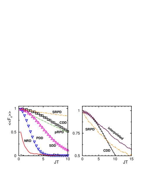
Figure 2: (color online) Deterministic vs. random DD based on a 4-pulse sequence for Hamiltonian (4) with $N=8$ in the logical-rotating frame. Average fidelity over $10^{2}$ control realizations, at $T_{n}=n|{\cal G}|\Delta t$. Left panel: $\Delta=1$, $\Delta t=0.1J^{-1}$. Free evolution: (black) dashed line at the bottom. Right panel: $\Delta=5$, $\Delta t=0.05J^{-1}$.

V Conclusions

We have reinforced the advantages of randomization in terms of faster convergence and long-time stabilization, by comparing the performance of various decoupling schemes in refocusing the evolution of a chain of nearest-neighbor-interacting qubits. Our analysis also indicates the promising role of stochasticity in the search of optimized pulse sequences. While preliminary results indicate that the main conclusions remain unchanged when pulse imperfections are considered, further analysis is needed in this direction. It is also our hope that these findings will prompt experimental verifications in available control devices.

VI Acknowledgements

We thank Oliver Kern for a careful reading of the manuscript and useful suggestions. L.V. thanks Victor S. Batista for the opportunity to attend and contribute to a PQE stimulating session on Multipulse Coherent Quantum Control. Partial support from Constance and Walter Burke through their Special Projects Fund in Quantum Information Science is gratefully acknowledged.

References

- (1) L. Gammaitoni, P. Hänggi, P. Jung, and F. Marchesoni, Rev. Mod. Phys. 70, 223 (1998).
- (2) V. Kendon and B. Tregenna, Phys. Rev. A 67, 042315 (2003).
- (3) A. Beige, Inst. Phys. Conf. Ser. 173, 35 (2003).
- (4) T. Prosen and M. Žnidarič, J. Phys. A 34, L681 (2001); ibid 35, 1455 (2002).
- (5) P. Hayden, D. Leung, P. W. Shor, and A. Winter, Commun. Math. Phys. 250, 371 (2004).
- (6) J. Emerson, Y. S. Weinstein, M. Saraceno, S. Lloyd, and D. G. Cory, Science 302, 2098 (2003).
- (7) L. Viola and E. Knill, Phys. Rev. Lett. 94, 060502 (2005).
- (8) O. Kern, G. Alber, and D. L. Shepelyansky, Eur. Phys. J. D 32, 153 (2005).
- (9) O. Kern and G. Alber, Phys. Rev. Lett. 95, 250501 (2005).
- (10) L. F. Santos and L. Viola, Phys. Rev. A 72 062303 (2005).
- (11) O. Kern and G. Alber, Phys. Rev. A 73 062302 (2005).
- (12) L. F. Santos and L. Viola, Phys. Rev. Lett. 97 150501 (2006).
- (13) U. Haeberlen and J. S. Waugh, Phys. Rev., 175, 453 (1968).
- (14) L. Viola and S. Lloyd, Phys. Rev. A 58, 2733 (1998).
- (15) L. Viola, E. Knill, and S. Lloyd, Phys. Rev. Lett. 82, 2417 (1999); L. Viola, Phys. Rev. A 66, 012307 (2002), and references therein.
- (16) L.-A. Wu and D. A. Lidar, Phys. Rev. Lett. 88, 207902 (2002).
- (17) R. R. Ernst, G. Bodenhausen, and A. Wokaun, Principles of Nuclear Magnetic Resonance in One and Two Dimensions (Oxford University Press, Oxford, 1994).
- (18) U. Haeberlen, High Resolution NMR in Solids: Selective Averaging (Academic Press, New York, 1976).
- (19) Note that the norm of the resulting effective Hamiltonian, , is of . In general, the -th order of DD is characterized by averaging accuracy of .
- (20) B. Schumacher, Phys. Rev. A 54, 2614 (1996).
- (21) M. A. Nielsen, Phys. Lett. A 303, 249 (2002).
- (22) E. M. Fortunato, L. Viola, J. Hodges, G. Teklemariam, and D. G. Cory, New J. Phys. 4, 5.1 (2002).
- (23) D. Loss and D. P. DiVincenzo, Phys. Rev. A 57, 120 (1998).
- (24) J. Baugh, O. Moussa, C. A. Ryan, R. Laflamme, C. Ramanathan, T. F. Havel, and D. G. Cory, Phys. Rev. A 73 022305 (2006)
- (25) M. I. Dykman and P. M. Platzman, Phys. Rev. B 64, 245309 (2001).
- (26) M. Stollsteimer and G. Mahler, Phys. Rev. A 64, 052301 (2001).
- (27) K. Khodjasteh and D. A. Lidar, Phys. Rev. Lett. 95, 180501 (2005).
- (28) P. Maunz, T. Puppe, I. Schuster, N. Syassen, P. W. H. Pinkse, and G. Rempe, Nature 428, 50 (2004); J. E. Reiner, W. P. Smith, L. A. Orozco, H. M. Wiseman, and J. Gambetta, Phys. Rev. A. 70, 023819 (2004).
- (29) A. Hopkins, K. Jacobs, S. Habib, and K. Schwab, Phys. Rev. B 68, 235328 (2003).
- (30) M. A. Armen, J. K. Au, J. K. Stockton, A. C. Doherty, and H. Mabuchi, Phys. Rev. Lett., 89, 133602 (2002); W. P. Smith, J. E. Reiner, L. A. Orozco, S. Kuhr, and H. M. Wiseman, Phys. Rev. Lett., 89, 133601 (2002); J. M. Geremia, J. K. Stockton, and H. Mabuchi, Science, 304, 270 (2004); P. Bushev, D. Rotter, A. Wilson, F. Dubin, C. Becher, J. Eschner, R. Blatt, V. Steixner, P. Rabl, and P. Zoller, Phys. Rev. Lett., 96, 043003 (2006).