Low-lying bifurcations in cavity quantum electrodynamics

Abstract

The interplay of quantum fluctuations with nonlinear dynamics is a central topic in the study of open quantum systems, connected to fundamental issues (such as decoherence and the quantum-classical transition) and practical applications (such as coherent information processing and the development of mesoscopic sensors/amplifiers). With this context in mind, we here present a computational study of some elementary bifurcations that occur in a driven and damped cavity quantum electrodynamics (cavity QED) model at low intracavity photon number. In particular, we utilize the single-atom cavity QED Master Equation and associated Stochastic Schrödinger Equations to characterize the equilibrium distribution and dynamical behavior of the quantized intracavity optical field in parameter regimes near points in the semiclassical (mean-field, Maxwell-Bloch) bifurcation set. Our numerical results show that the semiclassical limit sets are qualitatively preserved in the quantum stationary states, although quantum fluctuations apparently induce phase diffusion within periodic orbits and stochastic transitions between attractors. We restrict our attention to an experimentally realistic parameter regime.

I Introduction

Bifurcation analysis is a fundamental aspect of dynamical systems theory Stro01 ; Perk06 . It provides a powerful set of tools and concepts for the study of bistability, hysteresis and related phenomena in natural and engineered systems. In some practical applications the theory can be used to ensure operation in a structurally stable parameter range, while in others it is used to identify operating points that are highly sensitive to specific perturbations. The latter objective can arise in scenarios where, for example, one seeks to exploit the intrinsic nonlinear dynamics of a sensing device to provide amplification. This remarkably robust strategy applies even in nanomechanical Almo05 and single trapped-ion Tsen99 systems, as well as in superconducting circuit implementations of quantum computation Sidd04 . However, the role of quantum fluctuations in determining minimum noise figures and back-action for bifurcation amplifiers is not yet understood. It has also long been appreciated that bistability and hysteresis could provide a basis for designing logic devices for switching and computation in nonlinear optics Abra82 ; interest in this subject has been reinvigorated by advances in the fabrication of photonic bandgap structures and other integrated optical circuits Yani03 ; Prie05 . Implementations based on strong coupling to quantum dots may provide access to a technologically important regime of attojoule and picosecond switching, but such performance would seem to imply an energy separation between logical states on the order of tens of photons. Hence the role of quantum fluctuations again calls for attention. Bifurcation analysis and design thus have many roles to play in modern engineering and applied science, and there is a real need to incorporate stochastic analysis.

In recent years, there has been growing interest in studying bifurcation-like behavior of physical, chemical and biological systems that are fundamentally discrete and stochastic in nature but that can be well described in some relevant limit by nonlinear differential equations or maps. In chemical reactions, for example, ordinary differential rate equations (corresponding to the so-called law of mass action) provide an accurate model in the limit where the number of molecules per species becomes infinite (at fixed concentration) Gill77 . As a cell biologist or as an engineer designing reaction networks for molecular computation, however, one might well be concerned with understanding precisely how bifurcation phenomena predicted by the rate equations are reflected in the stochastic dynamics of a small number of reacting molecules. Stochastic extensions of rigorous bifurcation theory are now being developed by several authors Arno98 ; Zeem88 , but experimental and numerical investigations of specific systems are providing crucial guidance for early development of the field Elow00 ; Qian02 ; Steu04 .

Stochastic behavior and dynamic nonlinearity naturally coexist in the quantized setting of cavity quantum electrodynamics (cavity QED) with strong coupling RempeKimble91 ; Mabu02 . While the latter subject may seem a bit esoteric in comparison to chemical reaction networks, it has important connections to nonlinear-optical signal processing and offers the additional interest of incorporating quantum interference and atom-field entanglement. As in the case of chemical reactions, the microscopic equations of cavity QED are known to have a continuous and deterministic macroscopic limit (corresponding to many weakly-coupled atoms), which is related to elementary models of the laser. It was recognized even in the early days of cavity QED Sava88 that progress in the laboratory would eventually provide a means of exploring bifurcation phenomena such as optical bistability in a single-atom and few-photon regime; such experiments are indeed now feasible. An opportunity thus arises for the empirical study of bifurcation phenomena in the discrete physical limit, providing an intriguing quantum-optical counterpart to the systems mentioned above.

While previous theoretical Sava88 ; Kili91 ; Kozl99 and experimental Hood98 investigations of single-atom bistability have largely focused on steady-state observables of the transmitted optical field, we will here follow the spirit of Refs. Alsi91 ; Well01 in studying transient signals and stochastic jumps observable in the broadband photocurrent generated in individual experimental trials. We look in particular at a case of absorptive bistability, a supercritical Hopf bifurcation, and a subcritical Hopf bifurcation, all of which occur with mean intracavity photon numbers of order ten. Our principal aims in this paper are to illustrate a systematic approach (building upon Ref. GangNingHaken90 ; GNH90b ) to expanding the known inventory of bifurcation-type phenomena in single-atom cavity QED, and to highlight some conspicuous predictions of the fully quantum model as compared to the semiclassical Maxwell-Bloch Equations. In so doing we hope to begin to illumine a more comprehensive picture of the quantum-classical transition in cavity nonlinear optics Berm94 ; Mand97 , bridging what is generally known about linear-gaussian Wise05 and chaotic Habi06 open quantum systems Vard01 .

II The driven and damped Jaynes-Cummings model

II.1 Quantum Dynamical Description

We consider the driven Jaynes-Cummings Hamiltonian CarmichaelOpenSys which models the interaction of a single mode of an optical cavity having resonant frequency $\omega_{c}$, with a two-level atom, comprised of a ground state $|g\rangle$ and an excited state $|e\rangle$ separated by a frequency $\omega_{a}$. For an atom-field coupling constant $g_{0}$ and a drive field amplitude $\mathcal{E}$, the Hamiltonian written in a frame rotating at the drive frequency $\omega_{l}$ is given by [$\hbar=1$]:

$$\mathcal{H}=\Delta_{c}a^{{\dagger}}a+\Delta_{a}\sigma_{+}\sigma_{-}+ig_{0}(a^{{\dagger}}\sigma_{-}-a\sigma_{+})+i\mathcal{E}(a^{\dagger}-a)\ ,$$ (1)

where $\,\Delta_{a}=\omega_{a}-\omega_{l}\,$ and $\,\Delta_{c}=\omega_{c}-\omega_{l}\,$. In equation (1), $a$ is the field annihilation operator and $\sigma_{-}=|g\rangle\langle e|$ is the atomic lowering operator. In addition to the coherent dynamics governed by (1) there are two dissipative channels for the system: the atom may spontaneously emit into modes other than the preferred cavity mode, at a rate $\gamma_{\parallel}$, and photons may pass through the cavity output coupling mirror, at a rate $2\kappa$. Furthermore, we model the case of non-radiative dephasing (at rate $\gamma_{nr}$) between the atomic ground and excited states. In the analysis to follow, we will be concentrating solely on the situation where $\gamma_{nr}=0$, i.e. purely radiative damping; however, $\gamma_{nr}$ is included here to indicate that we are not restricted to this case (in particular, the parameterization employed in section III will imply a variable dephasing.) The unconditional master equation describing this driven, damped, and dephased evolution is

$$\dot{\rho} = -i[\mathcal{H},\rho]+\kappa(2a\rho a^{\dagger}-a^{\dagger}a\rho-\rho a^{\dagger}a)$$

$$+\ \gamma_{\parallel}/2(2\sigma_{-}\rho\sigma_{+}-\sigma_{+}\sigma_{-}\rho-\rho\sigma_{+}\sigma_{-})$$

$$+\ \gamma_{nr}/2(\sigma_{z}\rho\sigma_{z}-\rho)$$

where $\sigma_{z}=[\sigma_{+},\sigma_{-}]$ measures the population difference between the excited and ground states.

While $g_{0}$ measures the coherent coupling rate between the atom and the cavity, the rates $\gamma_{\parallel}$, $\gamma_{nr}$, and $\kappa$ characterize processes which tend to inhibit the build up of coherence. The qualitative nature of the dynamics (II.1) may be determined by two dimensionless parameters which measure the relative strengths of the coherent and incoherent processes: the critical photon number

$$n_{0}=\frac{\gamma_{\parallel}\gamma_{\perp}}{4g_{0}^{2}}\;,$$ (3)

and the critical atom number

$$N_{0}=\frac{2\gamma_{\perp}\kappa}{g_{0}^{2}}\;,$$ (4)

where $\gamma_{\perp}$ is the transverse relaxation rate given by $\gamma_{\perp}=\gamma_{\parallel}/2+\gamma_{nr}$. The critical photon number provides a measure of the number of photons needed to saturate the response of a single atom. Therefore, in the regime $n_{0}<1$, a single photon inside the resonator may induce a nonlinear system response. Similarly, the critical atom number roughly quantifies the number of atoms required to drastically change the resonant properties of the cavity. When $N_{0}<1$, a single atom inserted into the cavity will have a dramatic effect on the cavity output. The so-called “strong coupling regime” of cavity QED, which is usually used to denote the regime where the coherent coupling dominates over dissipation, is reached when the condition $(n_{0},N_{0})<1$ holds.

The master equation (II.1) may be used to find the time evolution for any operator acting on the system Hilbert space. In particular, it will be useful to know the dynamical equations for $\langle a\rangle$, $\langle\sigma_{-}\rangle$, and $\langle\sigma_{z}\rangle$ in order to make concrete comparisons with the semi-classical results that follow. Using the fact that $\dot{\langle O\rangle}=\mathrm{Tr}[O\dot{\rho}]$ for a system operator $O$, we obtain

$$\dot{\langle a\rangle} = -\kappa(1+i\Theta)\langle a\rangle+g_{0}\langle\sigma_{-}\rangle+\mathcal{E}$$

$$\dot{\langle\sigma_{-}\rangle} = -\gamma_{\perp}(1+i\Delta)\langle\sigma_{-}\rangle+g_{0}\langle a\sigma_{z}\rangle$$ (5)

$$\dot{\langle\sigma_{z}\rangle} = -\gamma_{\parallel}(\langle\sigma_{z}\rangle+1)-2g_{0}(\langle a^{\dagger}\sigma_{-}\rangle+\langle\sigma_{+}a\rangle)\;,$$

with $\gamma_{\perp}=\gamma_{\parallel}/2+\gamma_{nr}$, $\Theta=(\omega_{c}-\omega_{l})/\kappa$, and $\Delta=(\omega_{a}-\omega_{l})/\gamma_{\perp}$.

It should be noted that these formulae may be easily generalized to the case of $N$ non-interacting atoms each coupled to the same mode of the electromagnetic field, with coupling constant $g_{0}$. In this case, the Hamiltonian becomes

$$\mathcal{H}=\Delta_{c}a^{{\dagger}}a+\sum_{j=1}^{N}\Delta_{a}\sigma_{+}^{j}\sigma_{-}^{j}+\sum_{j=1}^{N}ig_{0}(a^{{\dagger}}\sigma_{-}^{j}-a\sigma_{+}^{j})+i\mathcal{E}(a^{\dagger}-a)\ ,$$ (6)

and the new master equation is

$$\dot{\rho} = -i[\mathcal{H},\rho]+\kappa(2a\rho a^{\dagger}-a^{\dagger}a\rho-\rho a^{\dagger}a)$$

$$+\ \gamma_{\parallel}/2\sum_{j=1}^{N}(2\sigma_{-}^{j}\rho\sigma_{+}^{j}-\sigma_{+}^{j}\sigma_{-}^{j}\rho-\rho\sigma_{+}^{j}\sigma_{-}^{j})$$

$$+\ \gamma_{nr}/2\sum_{j=1}^{N}(\sigma^{j}_{z}\rho\sigma^{j}_{z}-\rho)\ ,$$

where $\sigma_{-}^{j}$ is the lowering operator for the $j$th atom and $[\sigma_{+}^{j},\sigma_{-}^{k}]=\delta_{jk}\sigma_{z}^{j}$. The equations of motion for the operator expectations become

$$\dot{\langle a\rangle} = -\kappa(1+i\Theta)\langle a\rangle+g_{0}\sum_{j=1}^{N}\langle\sigma_{-}^{j}\rangle+\mathcal{E}$$

$$\dot{\langle\sigma_{-}^{j}\rangle} = -\gamma_{\perp}(1+i\Delta)\langle\sigma_{-}^{j}\rangle+g_{0}\langle a\sigma_{z}^{j}\rangle$$ (8)

$$\dot{\langle\sigma_{z}^{j}\rangle} = -\gamma_{\parallel}(\langle\sigma_{z}^{j}\rangle+1)-2g_{0}(\langle a^{\dagger}\sigma_{-}^{j}\rangle+\langle\sigma_{+}^{j}a\rangle)\;.$$

If we define $\ \sigma_{-}=\sum_{j=1}^{N}\sigma_{-}^{j}\$ and $\ \sigma_{z}=\sum_{j=1}^{N}\sigma_{z}^{j}\$ as the collective pseudo-spin operators, we arrive at the following set of dynamical equations

$$\dot{\langle a\rangle} = -\kappa(1+i\Theta)\langle a\rangle+g_{0}\langle\sigma_{-}\rangle+\mathcal{E}$$

$$\dot{\langle\sigma_{-}\rangle} = -\gamma_{\perp}(1+i\Delta)\langle\sigma_{-}\rangle+g_{0}\langle a\sigma_{z}\rangle$$ (9)

$$\dot{\langle\sigma_{z}\rangle} = -\gamma_{\parallel}(\langle\sigma_{z}\rangle+N)-2g_{0}(\langle a^{\dagger}\sigma_{-}\rangle+\langle\sigma_{+}a\rangle)\;.$$

Therefore, we may think of equation (9) as a description of the operator expectation dynamics for either a single-atom (with $N=1$) or multi-atom system. In either case, the coupled equations (9) are not closed, as they contain expectation values of operator products. Therefore, we also need the dynamical equations for the higher order moments, of which there are an infinite number. For purely optical systems, order parameters can often be identified so that a system size expansion can yield a finite, closed set of equations which are valid in the “low-noise” limit (when the order parameter is large). Unfortunately, for coupled atom-field systems, there exists no suitable choice of system scaling parameters which would justify a system size expansion CarmichaelOpenSys . Furthermore, it is known that the quantum fluctuations produced by optical bistability can be non-classical even when $N\gg 1$ RempeKimble91 , and therefore would not fit into the classical mold which is the basis of a system size expansion. Nevertheless it has been demonstrated Rose91 that the Maxwell-Bloch equations, which will be derived from (9) below, can be brought with some refinements into close agreement with experiments on absorptive optical bistability in a multi-atom system. Indeed said equations are generally accepted as a canonical, though somewhat phenomenological, model for cavity nonlinear optics outside the strong coupling regime Mand97 ; Lugiato .

II.2 Semi-Classical Description

An ad hoc (and somewhat crude) approach obtaining a closed set of equations from (9) is to simply factorize the operator products, e.g. $\langle a^{\dagger}\sigma_{-}\rangle\rightarrow\langle a^{\dagger}\rangle\langle\sigma_{-}\rangle$. While there is no formal basis for this procedure in general, the intuition behind it is that for a large system with many weakly-excited atoms, the atom-field correlations will tend to zero, allowing for expectations of operator products to be factorized Lugiato ; Carm86 . But it should be noted that this approximation is not justified in the case of strong driving and certainly not for a single atom. This factorization yields

$$\dot{\langle{a}\rangle} = -\kappa\left(1+i\Theta\right)\langle a\rangle+g_{0}\langle\sigma_{-}\rangle+\mathcal{E}$$

$$\dot{\langle\sigma_{-}\rangle} = -\gamma_{\perp}\left(1+i\Delta\right)\langle\sigma_{-}\rangle+g_{0}\langle a\rangle\langle\sigma_{z}\rangle$$ (10)

$$\dot{\langle\sigma_{z}\rangle} = -\gamma_{\parallel}\left(\langle\sigma_{z}\rangle+N\right)-2g_{0}(\langle a^{\dagger}\rangle\langle\sigma_{-}\rangle+\langle\sigma_{+}\rangle\langle a\rangle)$$

which are the well known the Maxwell-Bloch equations, used to describe the semi-classical evolution of a classical field coupled to an atomic medium. The atom-field correlations which were discarded in performing the factorization above will tend to contribute “noise” on top of the mean field evolution described by Eq. (10). To put these equation into a more common form, we make the following definitions:

$$\tilde{x}\doteq\langle a\rangle,\quad\tilde{p}\doteq\frac{2}{N}\langle\sigma_{-}\rangle,\quad\tilde{D}\doteq\frac{1}{N}\langle\sigma_{z}\rangle.$$ (11)

so that (10) becomes

$$\dot{\tilde{x}} = -\kappa(1+i\Theta)\tilde{x}+(Ng_{0}/2)\tilde{p}+\mathcal{E}$$

$$\dot{\tilde{p}} = -\gamma_{\perp}(1+i\Delta)\tilde{p}+2g_{0}\tilde{x}\tilde{D}$$ (12)

$$\dot{\tilde{D}} = -\gamma_{\parallel}(\tilde{D}+1)-g_{0}(\tilde{x}^{*}\tilde{p}+\tilde{p}^{*}\tilde{x})\ .$$

A computationally more practical form of (II.2), which will prove useful in the bifurcation analysis to follow, may be obtained by transforming it into a dimensionless set of equations. We first make the following change of variables

$$\tilde{x}\rightarrow\sqrt{n_{0}}\,x,\quad\tilde{p}\rightarrow-\sqrt{\frac{\gamma_{\parallel}}{\gamma_{\perp}}}\,p,\quad\tilde{D}\rightarrow-D,\quad$$ (13)

followed be a re-scaling of time

$$t\rightarrow t^{\prime}/\gamma_{\perp}\ ,$$ (14)

so that we are left with the dimensionless Maxwell-Bloch equations Lugiato :

$$\dot{x} = -k\left[(1+i\Theta)x+2Cp-y\right]$$

$$\dot{p} = -(1+i\Delta)p+xD$$ (15)

$$\dot{D} = -\gamma\left[D-1+(x^{*}p+p^{*}x)/2\right]$$

where the complex variables $x$ and $p$ represent the amplitude of the intra-cavity field and the normalized atomic polarization, respectively, $D$ is the (real) atomic population inversion, and $y$ is the amplitude of the external drive field. The cooperativity parameter, $C$, measures the strength of the collective atom-field interaction, while $k$ and $\gamma$ are, respectively, the cavity field decay and atomic spontaneous emission rates, scaled by the atomic transverse relaxation rate, $\gamma_{\perp}$:

$$\gamma=\frac{\gamma_{\parallel}}{\gamma_{\perp}},\quad k=\frac{\kappa}{\gamma_{\perp}},\quad C=\frac{Ng_{0}^{2}}{2\kappa\gamma_{\perp}},\quad y=\frac{\mathcal{E}}{\kappa\sqrt{n_{0}}}\ .$$ (16)

The two detuning parameters $\Theta$ and $\Delta$ are the same as in Eq. (5). Although there is no way to express the steady-state solutions for the dependent variables $x$, $p$, and $D$ in terms of the independent variables, we can find a simple set of equations relating the stationary solutions of the problem:

$$y = |x_{ss}|\left\{\left[1+\frac{2C}{1+\Delta^{2}+|x_{ss}|^{2}}\right]^{2}\right.$$ (17)

$$+\ \left.\left[\Theta-\frac{2C\Delta}{1+\Delta^{2}+|x_{ss}|^{2}}\right]^{2}\right\}^{1/2}\ ,$$

$$p_{ss} = \frac{(1-i\Delta)x_{ss}}{1+\Delta^{2}+|x_{ss}|^{2}}\ ,$$ (18)

$$D_{ss} = \frac{1+\Delta^{2}}{1+\Delta^{2}+|x_{ss}|^{2}}\ .$$ (19)

In Fig. 1 we plot a typical input-output curve generated using Eq. (17). Note that in the range $8.7\lesssim y\lesssim 11.1$ the curve displays absorptive bistability, with the lower and upper branches of the ‘S’-shaped curve supporting stable solutions (the dashed portion of the curve is unstable).

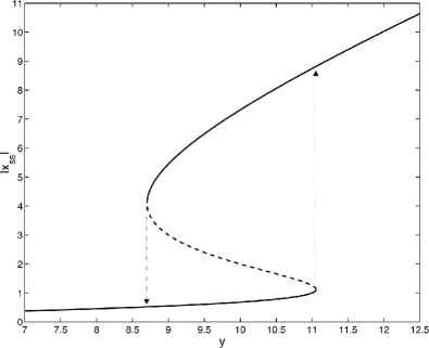
Figure 1: Semiclassical calculation of the intracavity steady-state field magnitude $|x_{ss}|$ versus drive field $y$. The dashed portion of the curve is unstable. The parameter values are: $C=10,k=0.1,\gamma=2,\Theta=0,$ and $\Delta=0.$ Arrows indicate the evolution of the steady-state solution when the drive field $y$ is swept smoothly through a bifurcation point: the state originally on the lower (upper) branch moving through the bifurcation point $y\approx 11.1$ ($y\approx 8.7$) is attracted to the upper (lower) branch.

It is important to note that the above equations depend upon $g_{0}$ and $N$ only through the cooperativity parameter, $C$. Thus, identical behavior is predicted for a range of systems with varying atom number and $g_{0}=\sqrt{2\kappa\gamma_{\perp}C/N}$. Of course, one expects that the quantum fluctuations and atom-field correlations that are disregarded in the derivation of the Maxwell-Bloch equations should begin to matter as $N$ approaches 1. A direct comparison of ‘system behavior’ according to (II.2) versus the master equation (II.1) with the quantities $\{\gamma,k,C,y,\Theta,\Delta\}$ held fixed can thus be construed as a case study in quantum-(semi)classical correspondence. The question of course is exactly what ‘system behavior’ should be compared and how; the strategy in what follows will be to focus on photocurrent properties near bifurcation points of the semiclassical model. We thus next discuss a systematic approach to finding interesting points in the bifurcation set of the Maxwell-Bloch equations, and then review a standard monte carlo approach to simulating photocurrents according to the quantum model. After presenting some numerical results, we conclude with a discussion of some interesting features of the quantum-semiclassical comparison that suggest directions for further research.

III Bifurcation set of the mean-field equations

In this section we delineate the process used to find and classify bifurcations in the mean-field dynamics described by Eq. (II.2). In particular, in Sec. III.1 we characterize both saddle-node bifurcations and Hopf bifurcations. We further differentiate between super- and subcritical Hopf bifurcations in Sec. III.2. In the former case, the bifurcation will destabilize a (typically) fixed point with a local (small amplitude) limit cycle born about the prior steady-state. In the latter case, no local limit cycle is created about the destabilized steady-state solution, and the system will move to a new (possibly distant) attractor. For this reason, subcritical Hopf bifurcations often lead to qualitatively more radical results, including regions of multi-stability.

III.1 Linearization about steady-state

In order to determine the parameter values that lead to bifurcations, we return to equation (II.2), and linearize the system dynamics about steady-state. We consider small fluctuations $\delta x,\delta p$, and $\delta D$ about steady-state, and set $x=x_{ss}+\delta x$, $p=p_{ss}+\delta p$, et cetera. After eliminating terms that are second order in the small fluctuations,

$$\left(\begin{array}[]{c}\dot{\delta x}\\ \dot{\delta x^{*}}\\ \dot{\delta p}\\ \dot{\delta p^{*}}\\ \dot{\delta D}\end{array}\right)=\mathbf{J}\left(\begin{array}[]{c}\delta x\\ \delta x^{*}\\ \delta p\\ \delta p^{*}\\ \delta D\end{array}\right)$$ (20)

where the Jacobian $\mathbf{J}$ is given by

$$\begin{split}\mathbf{J}&=\\ &-\left(\begin{array}[]{ccccc}k(1+i\Theta)&0&2Ck&0&0\\ 0&k(1-i\Theta)&0&2Ck&0\\ -D_{ss}&0&1+i\Delta&0&-x_{ss}\\ 0&-D_{ss}&0&1-i\Delta&-x_{ss}^{*}\\ \gamma p_{ss}^{*}/2&\gamma p_{ss}/2&\gamma x_{ss}^{*}/2&\gamma x_{ss}/2&\gamma\end{array}\right).\end{split}$$ (21)

The associated characteristic equation will have the form

$$\lambda^{5}+a_{1}\lambda^{4}+a_{2}\lambda^{3}+a_{3}\lambda^{2}+a_{4}\lambda+a_{5}=0$$ (22)

with coefficients given by the following expressions:

$$\begin{array}[]{lclclc}a_{1}&=&2+\gamma+2k\ ,\\ a_{2}&=&k^{2}(1+\Theta^{2})+(2\gamma+1+\Delta^{2}+\gamma|x_{ss}|^{2})\\ &&+\ 2k(\gamma+2)+4kCD_{ss}\ ,\\ a_{3}&=&\gamma(1+\Delta^{2}+|x_{ss}|^{2})+2k(2\gamma+1+\Delta^{2}+\gamma|x_{ss}|^{2})\\ &&+\ k^{2}(1+\Theta^{2})(\gamma+2)+4kCD_{ss}(\gamma+k+1)\\ &&-\ \gamma kC(p_{ss}^{*}x_{ss}+p_{ss}x_{ss}^{*})\ ,\\ a_{4}&=&2k\gamma(1+\Delta^{2}+|x_{ss}|^{2})\\ &&+\ k^{2}(1+\Theta^{2})(2\gamma+1+\Delta^{2}+\gamma|x_{ss}|^{2})\\ &&+\ 2kCD_{ss}[2k(1-\Delta\Theta)+2\gamma(k+1)+\gamma|x_{ss}|^{2}]\\ &&+\ \gamma kC\left[i(\Delta+k\Theta)(p_{ss}^{*}x_{ss}-p_{ss}x_{ss}^{*})\right.\\ &&-\ \left.(k+1)(p_{ss}^{*}x_{ss}+p_{ss}x_{ss}^{*})\right]+4k^{2}C^{2}D_{ss}^{2}\ ,\\ a_{5}&=&\gamma k^{2}\{4C^{2}D_{ss}[D_{ss}-(p_{ss}^{*}x_{ss}+p_{ss}x_{ss}^{*})2]\\ &&+\ (1+\Theta^{2})(1+\Delta^{2}+|x_{ss}|^{2})\\ &&+\ 4CD_{ss}(1-\Delta\Theta)\}\ .\end{array}$$ (23)

These coefficients may be further simplified by using the form of $D_{ss}$ found in (17) and the relations

$$i(p_{ss}x_{ss}^{*}-p_{ss}^{*}x_{ss}) = -2\Delta|x_{ss}|^{2}/(1+\Delta^{2}+|x_{ss}|^{2})$$

$$(p_{ss}x_{ss}^{*}+p_{ss}^{*}x_{ss}) = 2|x_{ss}|^{2}/(1+\Delta^{2}+|x_{ss}|^{2})\quad,$$

so that the $a$’s found in the characteristic equation are written explicitly in terms of six parameters: $C,k,\gamma,\Theta,\Delta,$ and $|x_{ss}|$.

Needless to say, it is impossible to solve for the eigenvalues of this system analytically. However, other methods that provide analytic tests of stability do exist. Most notably, the Routh-Hurwitz criterion provides a set of inequalities based on combinations of the $a^{\prime}s$ that can be used to determine stability. Unfortunately, this procedure is simply too general, and it is ill suited for the purpose of determining the boundaries of instability in terms of our controllable parameters. We can, however, make use of the Routh-Hurwitz criteria to find the following necessary conditions for stability Orozco89 ; HuYang88

$$a_{1},\ a_{2},\ a_{3},\ a_{4},\ a_{5}\ >\ 0\ .$$

Furthermore, at a Hopf bifurcation the system must have a pair of pure imaginary eigenvalues, $\lambda_{1,2}=\pm i\omega$. Demanding that the characteristic equation support these solutions establishes the following critical condition for a Hopf bifurcation

$$f=(a_{1}a_{2}-a_{3})(a_{3}a_{4}-a_{2}a_{5})-(a_{1}a_{4}-a_{5})^{2}=0\quad,$$ (24)

with $f>0$ providing another necessary condition for stability.

For the purpose of delineating the instability boundaries, the six inequalities

$$a_{1},\ a_{2},\ a_{3},\ a_{4},\ a_{5},\ f\ >\ 0$$ (25)

are not equally important. Starting from a stable region of the parameter space, there are only two ways for the steady-state solution to become unstable: (i) a single real eigenvalue passes through the origin and becomes positive; (ii) a pair of complex conjugate eigenvalues cross the imaginary axis (starting from the LHP). For case (i) the coefficient $a_{5}$ must change signs first, whereas for case (ii) it is $f$ that first changes sign. Therefore, if the goal is to determine the conditions for a known stable state to become unstable, there is no need to consider the other necessary conditions and all focus may be placed on $a_{5}$ and $f$. Furthermore, if we are only interested in Hopf Bifurcations, we can also ignore the $a_{5}>0$ condition, which determines the boundary for saddle-node bifurcations where the steady-state curve displays a turning point (this can be seen by noting that $d(y^{2})/d(|x_{ss}|^{2})\propto a_{5}$, so that $a_{5}<0$ indicates bistability.)

It should be noted again, that the inequalities (25) are only necessary conditions for stability, they are not sufficient. For example, the system could have one real negative eigenvalue, and two pairs of complex eigenvalues each with positive real parts, and still have $a_{1},a_{2},a_{3},a_{4},a_{5},f>0$. However, the stability condition $f>0$ can be made sufficient for a given region in parameter space if we can show that this region is ‘connected’ to a known stable region of the space (two regions of parameter space are ‘connected’ if there exists a continuous variation of the parameters that moves the system from one region, while retaining the sign of $a_{1},a_{2},a_{3},a_{4},a_{5},$ and $f$ through the entire path.) Thus, if we know that a particular region of parameter space (with $a_{1},a_{2},a_{3},a_{4},a_{5}>0$) is connected to a stable region, we know that $f$ can serve as a necessary and sufficient condition for the steady-state solution to undergo a Hopf bifurcation. Practically, all this means is that starting from a stable state, the first crossing of a surface $a_{5}=0$ ($f=0$), will drive the system unstable through a saddle-node (Hopf) bifurcation. Furthermore, the stability condition $f>0$ is quite reliable in practice, even when we can’t show connectedness to a stable region.

III.2 Super- and subcritical Hopf bifurcations

In order to determine whether a Hopf bifurcation is super- or subcritical, the eigenvalues and eigenvectors about the bifurcation point must first be found. Among the possible reasons for seeking one or the other kind are that supercritical Hopf bifurcations can be used for resonant nonlinear amplification of small periodic signals Wies86 , and subcritical Hopf bifurcations are likely to indicate the presence of limit cycles that coexist with other attractors. The latter type of scenario may give rise to observable ‘quantum jumps’ among non-fixed point attractors, which would be an interesting generalization of the predictions of Refs. Alsi91 ; Mabu98 . We thus believe that the theory for distinguishing super- and subcritical Hopf bifurcations merits an extended discussion. Note that our expressions below and in the Appendix correct some apparent misprints in Ref. GangNingHaken90 , with minor changes of notation.

At a Hopf bifurcation, the linearized system (21) has a pair of pure imaginary eigenvalues $\lambda_{1,2}=\pm i\omega$, with the frequency $\omega$ determined by

$$\omega^{2}=\frac{a_{1}a_{4}-a_{5}}{a_{1}a_{2}-a_{3}}.$$ (26)

Thus, the characteristic equation (22) can be factored as

$$(\lambda^{2}+\omega^{2})(\lambda^{3}+a_{1}\lambda^{2}+b_{2}\lambda+b_{3})=0$$ (27)

with

$$b_{2}=a_{4}/\omega^{2},\quad\mathrm{and}\quad b_{3}=a_{5}/\omega^{2}.$$ (28)

Solving for the other three eigenvalues yields

$$\begin{array}[]{ccc}\lambda_{3}&=&\nu w-p/(3\nu w)-a_{1}/3\\ \lambda_{4}&=&\nu^{*}w-p/(3\nu^{*}w)-a_{1}/3\\ \lambda_{5}&=&w-p/(3w)-a_{1}/3\end{array}$$ (29)

where the variables

$$\begin{array}[]{ccc}\nu&=&(-1+i\sqrt{3})/2\\ w&=&\left\{q/2+\sqrt{(q/2)^{2}+(p/3)^{3}}\right\}^{1/3}\\ q&=&-2a_{1}^{3}/27+a_{1}b_{2}/3-b_{3}\\ p&=&-a_{1}^{2}/3+b_{2}\end{array}$$ (30)

are determined from the solution to the cubic equation embedded in (27). Following the approach in GangNingHaken90 (and noting several corrections), the system eigenvectors, $\mathbf{\alpha_{i}}$, may be found in terms of the $\lambda_{i}$ by solving the linearized dynamics

$$\mathbf{J}\mathbf{\alpha_{i}}=\lambda_{i}\mathbf{\alpha_{i}}$$ (31)

where $\mathbf{J}$ is the Jacobian in (21). Expressing the results in terms of the $\lambda_{i}$, one arrives at

$$\mathbf{\alpha_{i}}=\left(\begin{array}[]{c}\exp{(i\phi_{i})}\\ \exp{(-i\phi_{i})}\\ -\exp{(i\phi_{i})}\left[k(1+i\Theta)+\lambda_{i}\right]/(2Ck)\\ -\exp{(-i\phi_{i})}\left[k(1-i\Theta)+\lambda_{i}\right]/(2Ck)\\ -\exp{(i\phi_{i})}\left\{2CD_{ss}k+\left(1+i\Delta+\lambda_{i}\right)\left[k(1+i\Theta)+\lambda_{i}\right]\right\}/(2Ckx)\end{array}\right)$$ (32)

where the phase factor, $\exp{(i\phi_{i})}$, is chosen to preserve symmetry in the components and is given by

$$e^{i\phi_{i}}=\sqrt{\frac{x\left\{2CD_{ss}k+(1-i\Delta+\lambda_{i})[k(1-i\Theta)+\lambda_{i}]\right\}}{x^{*}\left\{2CD_{ss}k+(1+i\Delta+\lambda_{i})[k(1+i\Theta)+\lambda_{i}]\right\}}}.$$ (33)

The set of eigenvectors, $\{\mathbf{\alpha_{i}}\}$, define a linear transformation of variables such that dynamical equations about steady-state contain no linear cross couplings. The old variables are related to the new variables through the relation

$$\mathbf{\delta q}\,=\widetilde{\alpha}\,\mathbf{z}$$ (34)

where $\widetilde{\alpha}=\left[\mathbf{\alpha_{1}\;\alpha_{2}\;\alpha_{3}\;\alpha_{4}\;\alpha_{5}}\right]$ is the transformation matrix comprised of the system eigenvectors, and $\mathbf{\delta q}=\{\delta x,\;\delta x^{*},\;\delta p,\;\delta p^{*},\;\delta D\}^{T}$ are the fluctuations about steady-state. Starting from the dynamical equations for the fluctuations about steady-state

$$\dot{\delta x} = -k\left[(1+i\Theta)\delta x+2C\delta p\right]$$

$$\dot{\delta x^{*}} = (\dot{\delta x})^{*}$$

$$\dot{\delta p} = -(1+i\Delta)\delta p+\delta x\delta D$$

$$+\ \left\{\delta xD_{ss}+x_{ss}\delta D\right\}$$

$$\dot{\delta p^{*}} = (\dot{\delta p})^{*}$$

$$\dot{\delta D} = -\gamma\left[\delta D+(\delta x^{*}\delta p+\delta p^{*}\delta x)/2\right]$$

$$+\ \left\{\gamma/2(\delta x^{*}p_{ss}+x_{ss}^{*}\delta p+p_{ss}^{*}\delta x+\delta p^{*}x_{ss})\right\},$$

the transformation of coordinates $\mathbf{z}=\widetilde{\beta}\,\mathbf{\delta q}$, with $\widetilde{\beta}=\widetilde{\alpha}^{-1}$, eliminates any linear coupling between variables

$$\dot{z}_{j} = \lambda_{j}z_{j}+\beta_{j3}\delta x\delta D+\beta_{j4}\delta x^{*}\delta D$$ (36)

$$\ -\ \gamma\beta_{j5}(\delta x^{*}\delta p+\delta x\delta p^{*})/2\ .$$

Finally, after utilizing the transformation (34), this equation may be expressed in terms of the “diagonalized” coordinates alone:

$$\dot{z}_{j} = \lambda_{j}z_{j}+\sum_{k,l=1}^{5}\left[\beta_{j3}\alpha_{1k}\alpha_{5l}+\beta_{j4}\alpha_{2k}\alpha_{5l}\right.$$ (37)

$$\left.-\ \gamma\beta_{j5}(\alpha_{2k}\alpha_{3l}+\alpha_{1k}\alpha_{4l})/2\right]z_{k}z_{l}\ .$$

Having converted the system into the form (37), the dynamics about a Hopf bifurcation may be reduced onto a center manifold Guckenheimer : since the system dynamics will be dominated by the “slow” variables, $z_{1}$ and $z_{2}$, the flow of the differential equation may be locally approximated on the surface generated by $z_{1}$ and $z_{2}$, with the “fast” variables, $z_{j=3,4,5}$, represented by a local graph $z_{j}=A_{j}(z_{1},z_{2})$. Furthermore, the local graph, $A_{j}(z_{1},z_{2})$, may be approximated by a power series expansion

$$z_{j}=a_{20}(j)z_{1}^{2}+a_{11}(j)z_{1}z_{2}+a_{02}(j)z_{2}^{2}+...\,,\;j=3,4,5\;,$$ (38)

so that the reduced dynamics may be approximated by

$$\dot{z}_{j}\approx 2i\omega a_{20}(j)z_{1}^{2}-2i\omega a_{02}(j)z_{2}^{2}+...\,,\;j=3,4,5\,.$$ (39)

The coefficients in (38) are determined by substituting equations (38) and (39) into the exact dynamics (37) and equating like powers in $z_{1}^{n}z_{2}^{m}$.

With aid of the local graph (38), the dynamics may be reduced onto the center coordinates associated with eigenvalues having zero real part:

$$\dot{z}_{1}=i\omega z_{1}+b_{20}(1)z_{1}^{2}+b_{11}(1)z_{1}z_{2}+b_{02}(1)z_{2}^{2}+b_{21}(1)z_{1}^{2}z_{2}+...$$ (40)

with $z_{2}=z_{1}^{*}$ near the Hopf bifurcation. Writing $z_{1}=u+iv$, with $\{u,v\}\in\mathbb{R}$, the reduced dynamics of the complex variable $z_{1}$ may be expressed by a set of real coupled equations

$$\begin{array}[]{lll}\dot{u}&=&-\omega v+F(u,v)\\ \dot{v}&=&\omega u+G(u,v)\end{array}\ ,$$ (41)

with $F$ and $G$ comprised of terms nonlinear in $u$ and $v$. It can be shown Guckenheimer , that there exists a smooth change of variables which will put equation (41) into the normal form

$$\begin{array}[]{lll}\dot{r}&=&\eta_{3}r^{3}+\eta_{5}r^{5}+...\\ \dot{\theta}&=&\omega+\epsilon_{2}r^{2}+\epsilon_{4}r^{4}+...\end{array}\ ,$$ (42)

with the stability of the bifurcation governed by the sign of $\eta_{3}$. For $\eta_{3}<0$ the bifurcation is supercritical, and a stable, small amplitude limit cycle is born about the newly destabilized steady-state. For $\eta_{3}>0$, the bifurcation is subcritical, and no such small amplitude cycle is created. In this case, the system may be thrown far away from the steady-state solution, onto either a limit cycle, a different branch of the steady-state curve, or some other attractor.

Remaining details of the calculation of $\eta_{3}$ are relegated to the Appendix.

IV Quantum signatures of bistability and limit cycles

In this section we briefly review some computational tools that can be used to search for evidence of the semiclassical attractors in the quantum model. In the following section we present numerical results in which these tools are applied at several interesting points in the semiclassical bifurcation set.

IV.1 Steady-state Q-function

The Q-function (for the intracavity optical field) Wall95 can be used to characterize the steady-state behavior of the driven atom-cavity system. The benefits of using the Q-function, over the other common quasi-probability distributions, are twofold. Firstly, the Q-function is positive-semidefinite, and is therefore better suited for making comparisons to classical probability distributions (such as the stationary distribution of a classical model with noise). Secondly, the value of the Q-function has a very simple interpretation in terms of coherent states $|\alpha\rangle$ of the intracavity field, since for any given density operator $\rho$ we have $Q(\alpha)=\langle\alpha|\rho|\alpha\rangle$. Thus $Q(\alpha)$ may strictly be thought of as a probability, which further lends to the utility of the Q-function as a tool for making comparisons between the quantum and semiclassical descriptions of the equilibrium behavior.

In practice we can find the steady-state density operator $\rho_{ss}$ of the master equation (II.1) simply by setting the terms on its right-hand side to zero and solving the resulting algebraic equation. We can then use $Q_{ss}(\alpha)=\langle\alpha|\rho_{ss}|\alpha\rangle$, where there is an implied partial trace over the atomic degrees of freedom.

One naively expects that the Q-function should be bimodal when atom-cavity parameters are chosen in a bistable region of the Maxwell-Bloch equations Sava88 . Likewise, the existence of a limit cycle should give rise to a ring-shaped Q-function. Below we will show examples of such features, but we will also want a method for visualizing any possible coherent dynamics or large fluctuations buried within these stationary distributions. For example we want to be able to show that a ringlike Q-function indicates an intracavity field amplitude that oscillates coherently, as opposed to randomly diffusing around the circle. In the case of bistability we would also like to see the switching timescale and to examine the sharpness of the switching events.

IV.2 Quantum Trajectories

To visualize dynamics in the quantum model in an experimentally-relevant way, we turn to the method of quantum trajectory simulations CarmichaelOpenSys ; Wise93a .

The master equation (II.1) generates predictions of the unconditioned state of the atom-cavity system. That is, the solutions $\rho(t)$ of the master equation represent the knowledge we can have of the evolving system state without utilizing the information obtainable via real-time measurements of the output fields (cavity transmission and atomic fluorescence). Hence we may gain further insight into the dynamics by considering quantum predictions regarding the photocurrents; fortunately, the same theory used to derive the master equation provides a powerful set of tools for statistically-faithful sampling of continuous measurement records CarmichaelOpenSys ; Wise93a , and tells us how to interpret them as real-time observations of the intracavity dynamics Bout06 . Here we will use such ‘quantum trajectory’ methods for monte carlo simulations of the photocurrent generated by homodyne detection of the cavity output field Wise93a .

For the case of homodyne detection of the output fields, the stochastic Schrödinger equation (SSE) governing the evolution of the (unnormalized) conditional state vector, $|\psi_{c}\rangle$, is given by

$$\begin{array}[]{lclclc}d|\psi_{c}\rangle&=&-i\left(\mathcal{H}-i\kappa a^{\dagger}a-i\gamma_{\perp}\sigma_{+}\sigma_{-}\right)|\psi_{c}\rangle+\\ &&\ \sqrt{2\kappa}ae^{i\phi_{1}}|\psi_{c}\rangle dQ_{1}+\\ &&\ \sqrt{2\gamma_{\perp}}\sigma_{-}e^{i\phi_{2}}|\psi_{c}\rangle dQ_{2}\ ,\end{array}$$ (43)

with the Hamiltonian, $\mathcal{H}$, given in Eq. (1), and the phase factor $e^{i\phi_{1,2}}$ determining the field quadrature being measured (e.g. $\phi_{1,2}=0$ for measurement of the amplitude quadrature and $\phi_{1,2}=-\pi/2$ for the phase quadrature.) The measured homodyne photocurrents, $I_{hom_{1,2}}=\frac{dQ_{1,2}}{dt}$, which are, respectively, the homodyne photocurrents associated with the cavity and atomic decay channels, are calculated using

$$dQ_{1}=\sqrt{2\kappa}\frac{\langle a^{\dagger}e^{-i\phi_{1}}+ae^{i\phi_{1}}\rangle_{c}}{\langle\psi_{c}|\psi_{c}\rangle}dt+dW_{1}\ ,$$ (44)

$$dQ_{2}=\sqrt{2\gamma_{\perp}}\frac{\langle\sigma_{+}e^{-i\phi_{2}}+\sigma_{-}e^{i\phi_{2}}\rangle_{c}}{\langle\psi_{c}|\psi_{c}\rangle}dt+dW_{2}\ ,$$ (45)

where $dW_{1,2}$ are independent Wiener increments satisfying $\langle dW\rangle=0$ and $\langle(dW)^{2}\rangle=dt$. Numerical integration of equations (43,44) are performed using the stochastic integration routine incorporated in the Quantum Optics Toolbox Tan99 for MATLAB.

In any practical experiment, full measurement of the atomic spontaneous emission is not actually feasible as this would require a detector covering nearly $4\pi$ steradians of solid angle. Fortunately, the cavity-output homodyne photocurrent $I_{hom_{1}}$ generated by monte carlo integration of the above SSE (considered on its own without any reference to the corresponding $I_{hom_{2}}$) is sampled from the same law as the photocurrent one would see in an experiment in which the atomic decay channel was not measured at all vanH05 . We therefore make use of such photocurrent simulations below in our discussion of single-atom bistability and Hopf bifurcations. One should appreciate however that the conditional state $|\psi_{c}\rangle$ propagated by the SSE is then merely an internal variable of the monte carlo simulation, and not something that could actually be reconstructed (in a recursive estimation sense) from just the cavity-output photocurrent. The best one could do along the latter lines, without assuming high-efficiency observation of the cavity decay channel, would be to utilize the corresponding stochastic master equation (SME) Wise93a as an optimal quantum filter Bout06 . Even in a purely theoretical discussion one would like to utilize the SME (as in Ref. Mabu98 ) to generate not only realistic photocurrent samples, but also the conditional quantum states that one could in principle generate from them via recursive filtering. Unfortunately such numerical procedures are very computationally intensive. As we find that adequate indications of the dynamics underlying bimodal and ringlike Q-functions are provided by the photocurrents alone, we have limited our efforts to SSE-based simulations.

V Numerical results

V.1 Absorptive bistability

In Fig. 1 we plot the steady-state intra-cavity field magnitude vs. drive field predicted by the (dimensionless) semi-classical equations (17) for the case of purely absorptive bistability ($\Theta=\Delta=0$). These parameter values correspond to $g=1.41,\kappa=.1,\gamma_{\parallel}=2,\Delta_{a}=0,\Delta_{c}=0$, in the master equation (II.1), and a saturation photon number, $n_{0}=0.25$. In Fig. 2 we plot the bimodal Q-function obtained from the steady solution to the master equation for a drive field $y=11.3$ ($\mathcal{E}=0.565$), chosen such that the integrated probabilities in each mode of the Q-function are approximately equal. While this Q-function indicates that the quantum dynamics show bistable behavior, it is interesting to note that the master equation produces this bimodal distribution for a drive field where the mean-field equations do not predict bistability (the lower branch in Fig. 1 disappears at $y\approx 11.1$). In fact, the Q-function distributions over most of the semi-classically bistable region are not bimodal, and only become so for $11\lesssim y\lesssim 11.5$.

In Fig. 3 we plot the photocurrent (44) corresponding to a measurement of the amplitude quadrature of the cavity output field. As expected, the field localization brought about by the continuous homodyne measurement causes the signal amplitude to switch, at stochastic intervals, between values consistent with the two peaks in $Q(\alpha)$.

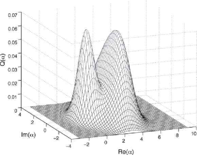
Figure 2: Steady-state $Q(\alpha)$ for the parameter values in Fig. 1, and drive field $y=11.3$.

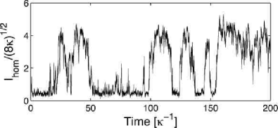
Figure 3: Homodyne photocurrent from quantum trajectory simulation for parameter values in Fig. 2.

V.2 Supercritical Hopf bifurcation

In Fig. 4 we plot the equilibrium attractors of the mean-field dynamics (II.2) for a case where the steady-state fixed points predicted in (17) undergo supercritical Hopf bifurcations. Starting on the lower (upper) branch of the steady-state curve, as the drive field $y$ is swept through the critical point $CP_{1}$ ($CP_{2}$) the fixed point is destabilized by a small amplitude limit cycle, $LC_{1}$, which grows in amplitude, peaking at $y\approx 2800$, until finally recombining with and restabilizing the fixed point at $CP_{2}$ ($CP_{1}$). To represent the oscillatory solution that is born out of the bifurcation, we plot the steady-state maximum field magnitude for a state localized on the stable limit cycle, and denote this as $LC_{1}$. Thus, the plotted curve $LC_{1}$ essentially represents the amplitude plus mean value of the limit cycle.

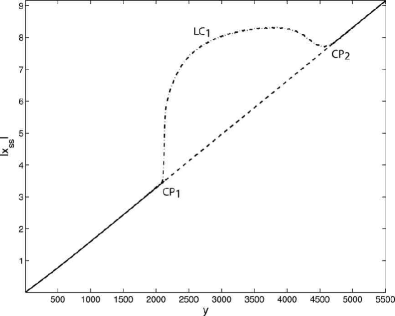
Figure 4: Semiclassical calculation of the intracavity steady-state field magnitude $|x_{ss}|$ versus drive field $y$. The parameter values are: $C=50,k=.01,\gamma=2,\Theta=-600$, and $\Delta=1.25.$ The upper dashed-dotted curve ($LC_{1}$)represents the steady-state oscillation maximum (steady-state magnitude plus mean value) associated with the limit cycle formed when the fixed point becomes unstable due to a Hopf bifurcation (at $CP_{1}$ and $CP_{2}$). The lower dashed curve is unstable.

The parameter values used in Fig. 4 correspond to $g=1,\kappa=.01,\gamma_{\parallel}=2,\Delta_{a}=1.25,\Delta_{c}=-6$ in Eq. (II.1), and a saturation photon number $n_{0}=0.5$. Using these values, we compute $Q(\alpha)$ for $y=2800$ ($\mathcal{E}=19.8$), where the limit cycle amplitude is maximal. The result is plotted in Fig. 5. The ring-like shape of the distribution is consistent with oscillation of a coherent state in the intracavity field. This interpretation is further supported by the inset in Fig. 6, where we plot the autocorrelation function $G_{Y}^{(1)}(\tau)=\langle Y(\tau)Y(0)\rangle-\langle Y(0)\rangle^{2}$, computed using the quantum regression theorem Wall95 , where $Y=\frac{i}{2}(a^{\dagger}-a)$ is the phase quadrature amplitude operator of the intracavity field. In addition, Fig. 6 displays the coherence time of the steady-state quantum oscillations over a range of drive fields. The results indicate that the coherence times depend strongly on the amplitude of the limit cycle, $LC_{1}$, which is again consistent with the idea of an oscillating coherent state for the intracavity field.

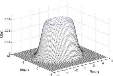
Figure 5: Steady-state $Q(\alpha)$ for the parameter values in Fig. 4, and drive field $y=2800$.

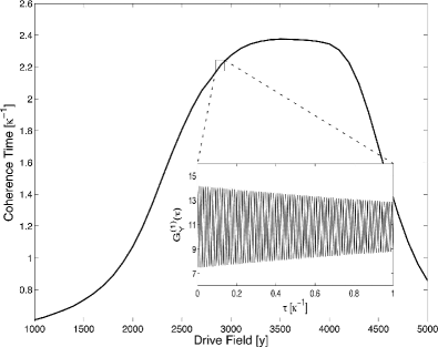
Figure 6: Coherence times calculated from steady-state autocorrelation function, $G_{Y}^{(1)}(\tau)$, of the quantum mechanical phase quadrature. Parameter values same as in Fig. 4. The coherence time is estimated by fitting a damped sinusoid to $G_{Y}^{(1)}(\tau)$. Inset: simulated $G_{Y}^{(1)}(\tau)$ for the drive field in Fig. 5.

It can be seen clearly from the inset of Fig. 6 that the limit cycle comprises an oscillation of the intracavity field at a frequency much higher than $\kappa$. It should thus be difficult to see the oscillation directly in the broadband photocurrent generated by amplitude-quadrature homodyne detection of the cavity output field. In Fig. 7 however we plot several power spectra of photocurrent records generated in quantum trajectory simulations. For $y=1000$ (below $CP_{1}$ in Fig. 4) the spectrum shows little or no sign of a coherent peak, but for $y=2800$ we see that homodyne detection of the field amplitude reveals clear evidence of the limit-cycle oscillation. This demonstrates at least a basic correspondence with the semiclassical predictions shown in Fig. 4. At $y=5000$ (above $CP_{2}$ in Fig. 4), however, we see that the quantum model still exhibits strong oscillations even though the semiclassical model predicts a fixed point solution. This persistence of the oscillatory behavior at both higher and lower driving fields can also be seen in Fig. 6.

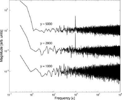
Figure 7: Power spectra computed from simulated photocurrents for amplitude-quadrature homodyne detection of the cavity output field, using parameter values as in Fig. 4. Lowest plot: $y=1000$, below the bifurcation point; middle plot: $y=2800$, where the classical oscillation amplitude is maximal; upper plot: $y=5000$, where the semiclassical model no longer predicts a limit cycle.

V.3 Subcritical Hopf bifurcation

In Fig. 8 we plot the steady-state solutions for a parameter regime where the mean-field equations predict a subcritical Hopf bifurcation. The solid (dashed) curve corresponds to the stable (unstable) fixed points predicted by Eq. (17), whereas the attractor $LC_{2}$ (plotted dashed-dotted) corresponds to a stable limit cycle. Beginning on the upper stable branch of fixed points, as the drive field is swept through the critical point $CP_{4}$, the system undergoes a subcritical Hopf bifurcation. In the range $475\lesssim y\lesssim 925$, the semiclassical equations predict coexistence of a stable fixed point and limit cycle, which is a common signature of subcritical bifurcations. Note that at $y\approx 925$ the limit cycle $LC_{2}$ is destabilized but the fixed point is not. The two arrowed lines in Fig. 8 do not represent solutions to the equations, but simply indicate which attractor a destabilized state will seek.

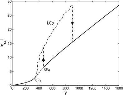
Figure 8: Semiclassical calculation of the intracavity steady-state field magnitude $|x_{ss}|$ versus drive field $y$. The parameter values are: $C=200,k=.05,\gamma=2,\Theta=-55,$ and $\Delta=2$. The upper dashed-dotted curve ($LC_{2}$) represents the steady-state oscillation maximum (steady-state magnitude plus mean value) associated with the limit cycle formed when the fixed point becomes unstable due to a Hopf bifurcation. The critical point $CP_{3}$ is supercritical, whereas the point $CP_{4}$ is subcritical. Note the coexistence of a stable fixed point and limit cycle in the range $475\lesssim y\lesssim 925$. The lower dashed curve is unstable.

The parameter values used in Fig. 8 correspond to $g=4.47,\kappa=.05,\gamma_{\parallel}=2,\Delta_{a}=2,\Delta_{c}=-2.75$, and a saturation photon number $n_{0}=0.025$. The small size of $n_{0}$ indicates that the qualitative behavior of steady-state solutions to the master equation will be dominated by quantum fluctuations (over the dynamics implied by the mean field equations.) We see that this interpretation is justified by the plot of $Q(\alpha)$ in Fig. 9, at a drive field $y=1000$, near the amplitude maximum of $LC_{2}$. The features in the surface plot (Fig. 9a) are hardly profound. The contour plot in Fig. 9b is somewhat more elucidating, and shows signs of the coexistence of oscillatory, albeit asymmetric, and fixed coherent states. These ‘blurry’ results are not surprising, as the small $n_{0}$, and relation (13), imply that, in the quantum case, the structure implied by the limit cycle and fixed points in Fig. 8 should be heavily affected by fluctuations.

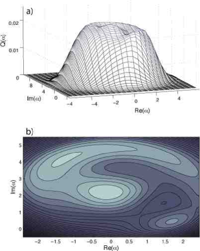
Figure 9: Steady-state surface (a) and contour plots (b) of $Q(\alpha)$ for the parameter values in Fig. 8, and drive field $y=1000$.

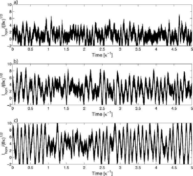
Figure 10: Homodyne photocurrent from quantum trajectory simulations with parameter values in Fig. 8. (a) drive field $y=500$, near the subcritical bifurcation point; (b) for drive field $y=1000$, near the oscillation amplitude maximum; (c) for drive field $y=1400$, beyond the region of semiclassical bistability.

Fig. 10 suggests, however, that the field localization provided by continuous homodyne measurement of the phase quadrature can reveal signatures of bistability in the photocurrent. In particular, in Fig. 10b we plot a typical trajectory for a drive field $y=1000$, as in Fig. 9. While the contrast is marginal, as it would have to be given the discussion above, the qualitative appearance of this simulated photocurrent record is that of oscillations interrupted by brief periods of stationary noise (which one could attribute to transient localization on the fixed point). Such intermittency can also be seen in Fig. 10c, which corresponds to a drive field, $y=1400$, well past the semiclassical region of multi-stability.

VI Conclusions

In this paper we have considered bifurcation phenomena as focal points for the investigation of quantum-(semi)classical correspondence in cavity nonlinear optics. We presented a general approach to the characterization of interesting points in the semiclassical (Maxwell-Bloch) bifurcation set, starting from the formal methods of Refs. GangNingHaken90 ; GNH90b (but with corrections to some of their equations as printed) and incorporating numerical simulations of the cavity QED master equation and (homodyne) stochastic Schrödinger equation. This approach leads to the prediction of self-oscillation and bifurcation-type behavior in an experimentally accessible parameter regime for single-atom cavity QED, under driving conditions in which the mean intracavity photon number is of order ten. It is interesting to see that such a wide range of input-output characteristics are supported in such a small state space.

The results of our numerical simulations point to a number of questions for further study. For example one would like to understand, in physical terms, what determines the correlation timescales found in Fig. 3 (bistability) and Fig. 6 (stable limit cycle). In scenarios where switching occurs between output-signal characteristics associated with different semiclassical attractors (as in Fig. 3 and Fig. 10), one would also like to know what determines the attractors’ relative stability and how the switching events are initiated (in the sense of Refs. Alsi91 ; Mabu98 ; Well01 ; vanH05 ). Can we understand the physical dynamics that give rise to limit-cycles in single-atom cavity QED (as in Ref. Alsi91 ), and why they are destabilized in subcritical Hopf bifurcations? Such investigations could be taken as a starting point for the development of quantum feedback control strategies Dohe00 ; vanHIEEE to stabilize desired fixed points Mack93 ; Yaow99 or limit cycles, or for inducing switching between them with minimum time or dissipated energy (as would be required for the types of optical signal processing applications mentioned in the introduction). More generally, one can ask about the applicability of ideas from classical bifurcation control Abed86 ; Chen00 . In this context, single-atom cavity QED provides an interesting model system for investigations of quantum feedback control far beyond the linear-gaussian regime Wise05 ; Stoc04a .

Returning finally to the issue of correspondence, one curious detail of our simulation results is that near hysteresis loops, bimodal behavior in the quantum model is often seen to persist well above (at higher driving fields than) the upper switching points of the Maxwell-Bloch equations, where saddle-node or subcritical bifurcations occur. We have also seen a case (supercritical Hopf) in which oscillatory behavior occurs over a wider parameter range than is predicted by the semiclassical model. It is certainly possible that these effects may be explainable by analogy with noise-induced ‘postponement’ Robi85 ; Fron87 , ‘advancement’ or ‘precursors’ Wies85 in classical nonlinear systems, or with some other known effect in classical random dynamics Hors84 ; Arno92 ; Arno99 ; Wack99 . If this is the case, it will be interesting to see what clues such analogies provide towards the development of physically-motivated stochastic extensions of the Maxwell-Bloch equations that can capture global (in the dynamical systems sense) effects of quantum fluctuations (thus going beyond what is possible with local-linearization approaches, as in Ref. CarmichaelNoAdiabatic ). In any case it will be natural to try to relate the machinery of ‘P-bifurcation’ analysis Arno98 ; Zeem88 to our steady-state Q-functions. Of course if sensible analogies with postponement in classical noise-driven systems cannot be established, it will be tempting to ask whether coherence or atom-field entanglement play any significant role in these or any other cavity QED bifurcation phenomena.

In any case, we certainly expect that further study of bifurcation phenomena in single-atom cavity QED will improve our understanding of the way that quantum fluctuations ‘enrich’ the mean-field phase portrait of coherent nonlinear dynamical systems.

Appendix A Calculation of $\eta_{3}$

The critical parameter $\eta_{3}$ can be expressed explicitly Guckenheimer ; Ning88 in terms of the coefficients in (40) and the bifurcation frequency $\omega$

$$\eta_{3}=\mathrm{Re}[b_{21}(1)]-\frac{1}{\omega}\mathrm{Im}[b_{20}(1)b_{11}(1)]\;.$$ (46)

As the calculations for the relevant coefficients are rather tedious and time consuming, they are included here for posterity:

$$\begin{array}[]{lll}a_{20}(j)&=&b_{20}(j)/(2i\omega-\lambda_{j})\;,\\ a_{11}(j)&=&-b_{11}(j)/\lambda_{j}\;,\end{array}\bigg{\}}\;j=3,4,5$$ (49)

where

$$b_{20}(j) = \beta_{j3}\alpha_{11}\alpha_{51}+\beta_{j4}\alpha_{21}\alpha_{51}$$ (50)

$$-\ \gamma\beta_{j5}(\alpha_{21}\alpha_{31}+\alpha_{11}\alpha_{41})/2\ ,$$

$$b_{11}(j) = \beta_{j3}\left(\alpha_{11}\alpha_{52}+\alpha_{12}\alpha_{51}\right)$$ (51)

$$+\ \beta_{j4}\left(\alpha_{21}\alpha_{52}+\alpha_{22}\alpha_{51}\right)$$

$$-\ \gamma\beta_{j5}\left[\alpha_{21}\alpha_{32}+\alpha_{22}\alpha_{31}\right.$$

$$+\ \left.\alpha_{11}\alpha_{42}+\alpha_{12}\alpha_{41}\right]/2\;.$$

Inserting (38), with coefficient $a_{20}(j)$ and $a_{11}(j)$ given by (49), into the diagonalized equation (37) for $j=1$ yields an expression for the last required coefficient

$$\begin{array}[]{lll}b_{21}(1)&=&\beta_{13}[a_{20}(3)\left(\alpha_{12}\alpha_{53}+\alpha_{13}\alpha_{52}\right)+a_{20}(4)\left(\alpha_{12}\alpha_{54}+\alpha_{14}\alpha_{52}\right)+a_{20}(5)\left(\alpha_{12}\alpha_{55}+\alpha_{15}\alpha_{52}\right)+\\ &&\quad a_{11}(3)\left(\alpha_{11}\alpha_{53}+\alpha_{13}\alpha_{51}\right)+a_{11}(4)\left(\alpha_{11}\alpha_{54}+\alpha_{14}\alpha_{51}\right)+a_{11}(5)\left(\alpha_{11}\alpha_{55}+\alpha_{15}\alpha_{51}\right)]\\ &+&\beta_{14}[a_{20}(3)\left(\alpha_{22}\alpha_{53}+\alpha_{23}\alpha_{52}\right)+a_{20}(4)\left(\alpha_{22}\alpha_{54}+\alpha_{24}\alpha_{52}\right)+\\ &&\quad\quad a_{20}(5)\left(\alpha_{22}\alpha_{55}+\alpha_{25}\alpha_{52}\right)+a_{11}(3)\left(\alpha_{21}\alpha_{53}+\alpha_{23}\alpha_{51}\right)+\\ &&\quad\quad\quad a_{11}(4)\left(\alpha_{21}\alpha_{54}+\alpha_{24}\alpha_{51}\right)+a_{11}(5)\left(\alpha_{21}\alpha_{55}+\alpha_{25}\alpha_{51}\right)]\\ &-&\frac{\gamma}{2}\beta_{15}[a_{20}(3)\left(\alpha_{22}\alpha_{33}+\alpha_{23}\alpha_{32}+\alpha_{12}\alpha_{43}+\alpha_{13}\alpha_{42}\right)+\\ &&\quad\quad\quad a_{20}(4)\left(\alpha_{22}\alpha_{34}+\alpha_{24}\alpha_{32}+\alpha_{12}\alpha_{44}+\alpha_{14}\alpha_{42}\right)+\\ &&\quad\quad\quad\quad a_{20}(5)\left(\alpha_{22}\alpha_{35}+\alpha_{12}\alpha_{45}+\alpha_{25}\alpha_{32}+\alpha_{15}\alpha_{42}\right)+\\ &&\quad\quad\quad\quad\quad a_{11}(3)\left(\alpha_{21}\alpha_{33}+\alpha_{11}\alpha_{43}+\alpha_{23}\alpha_{31}+\alpha_{13}\alpha_{41}\right)+\\ &&\quad\quad\quad\quad\quad\quad a_{11}(4)\left(\alpha_{21}\alpha_{34}+\alpha_{11}\alpha_{44}+\alpha_{24}\alpha_{31}+\alpha_{14}\alpha_{41}\right)+\\ &&\quad\quad\quad\quad\quad\quad\quad a_{11}(5)\left(\alpha_{21}\alpha_{35}+\alpha_{11}\alpha_{45}+\alpha_{25}\alpha_{31}+\alpha_{15}\alpha_{41}\right)]\;.\end{array}$$ (52)

References

- (1) S. H. Strogatz, Nonlinear Dynamics and Chaos: With Applications to Physics, Biology, Chemistry and Engineering (Westview Press, 2001).
- (2) L. Perko, Differential Equations and Dynamical Systems, 3rd. Edition, (Springer-Verlag, New York, 2006).
- (3) R. Almog, S. Zaitsev, O. Shtempluck and E. Buks, cond-mat/0511587.
- (4) C. H. Tseng, D. Enzer, G. Gabrielse and F. L. Walls, Phys. Rev. A 59, 2094 (1999).
- (5) I. Siddiqi, R. Vijay, F. Pierre, C. M. Wilson, M. Metcalfe, C. Rigetti, L. Frunzio and M. H. Devoret, Phys. Rev. Lett. 93, 207002 (2004).
- (6) E. Abraham and S. D. Smith, Rep. Prog. Phys. 45, 815 (1982).
- (7) M. F. Yanik, S. Fan, M. Soljac̆ić and J. D. Joannopoulos, Opt. Lett. 28, 2506 (2003).
- (8) G. Priem, P. Dumon, W. Bogaerts, D. Van Thourhout, G. Morthier and R. Baets, Opt. Express 13, 9623 (2005).
- (9) D. T. Gillespie, J. Phys. Chem. 81, 2340 (1977).
- (10) L. Arnold, Random Dynamical Systems (Springer-Verlag, Berlin, 1998).
- (11) E. C. Zeeman, Nonlinearity 1, 115 (1988).
- (12) M. B. Elowitz and S. Leibler, Nature 403, 335 (2000).
- (13) H. Qian, S. Saffarian and E. L. Elson, Proc. Nat. Acad. Sci. USA 99, 10376 (2002).
- (14) R. Steuer, J. T. Biol. 228, 293 (2004).
- (15) G. Rempe, R. J. Thompson, R.J. Brecha, W.D. Lee, and H.J. Kimble, Phys. Rev. Lett. 67 1727 (1991).
- (16) H. Mabuchi and A. C. Doherty, Science 298, 1372 (2002).
- (17) C. M. Savage and H. J. Carmichael, IEEE J. Quantum Electron. 24, 1495 (1988).
- (18) S. Ya. Kilin and T. B. Krinitskaya, J. Opt. Soc. Am. B 8, 2289 (1991).
- (19) A. V. Kozlovskii and A. N. Oraevskii, J. Expt. Theor. Phys. 88, 1095 (1999).
- (20) C. J. Hood, M. S. Chapman, T. W. Lynn and H. J. Kimble, Phys. Rev. Lett. 80, 4157 (1998).
- (21) P. Alsing and H. J. Carmichael, Quantum Opt. 3, 13 (1991).
- (22) T. Wellens and A. Buchleitner, Chemical Physics 268, 131 (2001).
- (23) H. Gang, C. Z. Ning, H. Haken, Phys. Rev. A 41, 2702 (1990).
- (24) H. Gang, C. Z. Ning, H. Haken, Phys. Rev. A 41, 3975 (1990).
- (25) P. R. Berman, ed., Cavity Quantum Electrodynamics (Academic Press, 1994).
- (26) P. Mandel, Theoretical Problems in Cavity Nonlinear Optics (Cambridge University Press, Cambrdige, 1997).
- (27) H. M. Wiseman and A. C. Doherty, Phys. Rev. Lett. 94, 070405 (2005).
- (28) S. Habib, K. Jacobs and K. Shizume, Phys. Rev. Lett. 96, 010403 (2006).
- (29) For a complementary perspective, see A. Vardi and J. R. Anglin, Phys. Rev. Lett. 86, 568 (2001).
- (30) H.J. Carmichael, An Open Systems Approach to Quantum Optics (Springer-Verlag, Berlin, 1993).
- (31) A. T. Rosenberger, L. A. Orozco, H. J. Kimble and P. D. Drummond, Phys. Rev. A 43, 6284 (1991).
- (32) L.A. Lugiato, in Progress in Optics, edited by E. Wolf (North-Holland, Amsterdam, 1984), Vol. XXI.
- (33) H. J. Carmichael, “Theory of quantum fluctuations in optical bistability,” in Frontiers in Quantum Optics, E. R. Pike and S. Sarkar, eds. (Adam Hilger, Bristol, 1986).
- (34) L.A. Orozco, H.J. Kimble, A.T. Rosenberger, L.A. Lugiato, M.L. Asquini, M. Brambilla, and L.M. Narducci, Phys. Rev. A 39, 1235 (1989).
- (35) G. Hu and G.J. Yang, Phys. Rev. A 38, 1979 (1988).
- (36) K. Wiesenfeld and B. McNamara, Phys. Rev. A 33, 629 (1986); K. A. Shore, J. Opt. Soc. Am. B 5, 1211 (1988); V. M. Eguíluz, M. Ospeck, Y. Choe, A. J. Hudspeth and M. O. Magnasco, Phys. Rev. Lett. 84, 5232 (2000).
- (37) H. Mabuchi and H. M. Wiseman, Phys. Rev. Lett. 81, 4620 (1998); misprint corrected in Phys. Rev. Lett. 82, 1798 (1999).
- (38) J. Guckenheimer and P. Holmes, Nonlinear Oscillations, Dynamical Systems, and Bifurcations of Vector Fields (Spring Verlag, New York, 1983).
- (39) D. F. Walls and G. J. Milburn, Quantum Optics (Springer, 1995).
- (40) H. M. Wiseman and G. J. Milburn, Phys. Rev. A 47, 642 (1993).
- (41) L. Bouten, R. van Handel and M. R. James math.OC/0601741.
- (42) S.M. Tan, J. Opt. B: Quant. Semiclass. Opt. 1, 424 (1999).
- (43) R. van Handel and H. Mabuchi, J. Opt. B: Quantum Semiclass. Opt. 7, S226 (2005).
- (44) A. C. Doherty, S. Habib, K. Jacobs, H. Mabuchi and S. M. Tan, Phys. Rev. A 62, 012105 (2000).
- (45) R. van Handel, J. K. Stockton and H. Mabuchi, IEEE Trans. Automat. Contr. 50, 768 (2005).
- (46) B. Macke, J. Zemmouri and N. E. Fettouhi, Phys. Rev. A 47, R1609 (1993).
- (47) L. Yaowen, P. Huican, Z. Hong and W. Yinghai, Phys. Lett. A 262, 416 (1999).
- (48) E. H. Abed and J. H. Fu, Systems and Controls Letters 7, 11 (1986).
- (49) G. Chen, J. L. Moiola and H. O. Wang, International Journal of Bifurcation and Chaos 10, 511 (2000).
- (50) J. K. Stockton, JM Geremia, A. C. Doherty and H. Mabuchi, Phys. Rev. A 69, 032109 (2004).
- (51) S. D. Robinson, F. Moss and P. V. E. McClintock, J. Phys. A: Math. Gen. 18, L89 (1985).
- (52) L. Fronzoni, R. Mannella, P. V. E. McClintock and F. Moss, Phys. Rev. A 36, 834 (1987).
- (53) K. Wiesenfeld, J. Stat. Phys. 38, 1071 (1985).
- (54) W. Horsthemke and R. Lefever, Noise-Induced Transitions: Theory and Applications in Physics, Chemistry and Biology (Springer, 1984).
- (55) L. Arnold and P. Boxler, in M. A. Pinsky, V. Wihstutz, eds. Diffusion Processes and Related Problems in Analysis, Volume II (Birkhäuser, Boston, 1992).
- (56) L. Arnold, G. Bleckert and K.-R. Schenk-Hoppé, in H. Crauel and M. Grundlach, eds., Stochastic Dynamics (Springer-Verlag, New York, 1999).
- (57) R. Wackerbauer, Phys. Rev. E 59, 2872 (1999).
- (58) H.J. Carmichael, Phys. Rev. A 33, 3262 (1986).
- (59) C.Z. Ning, J. Phys. A: Math. Gen. 21, L491 (1988).