Geometric phases and criticality in spin systems

Abstract

Berry phases, critical phenomena, XY model

A general formalism of the relation between geometric phases produced by circularly evolving interacting spin systems and their criticality behavior is presented. This opens up the way for the use of geometric phases as a tool to study regions of criticality without having to undergo a quantum phase transition. As a concrete example a spin-1/2 chain with XY interactions is presented and the corresponding geometric phases are analyzed. The generalization of these results to the case of an arbitrary spin system provides an explanation for the existence of such a relation.

1 Introduction

A few conceptual advances in quantum physics have been as exciting or as broadly studied as geometric phases. They lie within the heart of quantum mechanics giving a surprising connection between the geometric properties of evolutions and their dynamics. Historically, the first such effect was presented by Aharonov & Bohm (1959), where the quantum state of a charged particle acquires a phase factor when it moves along a closed path in the presence of a magnetic field. Since then a series of similar effects have been considered and experimentally verified. A more intriguing case where a quantum state is changed in a circular fashion was studied by Berry (1984) which led to the generation of the celebrated Berry phase. This effect does not need the presence of electromagnetic interactions and due to its abstract and general nature has found many applications (Shapere et al. 1989; Bohm et al. 2003).

A characteristic that all non-trivial geometric evolutions have in common is the presence of non-analytic points in the energy spectrum. At these points the state of the system is not well defined due to their degenerate nature. One could say that the generation of a geometric phase is a witness of such singular points. Indeed, the presence of degeneracy at some point is accompanied by curvature in its immediate neighborhood and a state that is evolved along a closed path is able to detect it. These points or regions, are of great interest to condensed matter or molecular physicists as they determine, to a large degree, the behavior of complex quantum systems. The geometric phases are already used in molecular physics to probe the presence of degeneracy in the electronic spectrum of complex molecules. Initial considerations by Herzberg and Longuet-Higgins (1963), revealed a sign reversal when a real Hamiltonian is continuously transported around a degenerate point. Its generalization to the complex case was derived by Stone (1976) and an optimization of the real Hamiltonian case was performed by Johansson & Sjöqvist (2004).

Geometric phases have been associated with a variety of condensed matter and solid state phenomena (Thouless et al. 1982; Resta 1994; Nakamura & Todo 2002; Ryu & Hatsugai 2006). Nevertheless, their connection to quantum phase transitions has only been shown recently by Carollo & Pachos (2005). It was farther elaborated by Zhu (2005), where the critical exponents were evaluate from the scaling behavior of geometric phases, and by Hamma (2006), who showed that geometric phases can be used as a topological test to reveal quantum phase transitions. In essence, quantum phase transitions describe the abrupt changes on the macroscopic behavior of a system resulting from small variations of external parameters. These critical changes are caused by the presence of degeneracies in the energy spectrum and are characterized by long range quantum correlations. This is an exciting area of research that considers a variety of effects such as the quantum Hall effect and high $T_{c}$ superconductivity.

Here we exploit geometric phases as a tool to probe quantum phase transitions in many-body systems. This provides the means to detect, not only theoretically, but also experimentally the presence of criticalities. Apart from the academic interest this approach may have certain advantages. In particular, the geometric evolutions do not take the system through a quantum phase transition. The latter is hard to physically implement as it is accompanied by multiple degeneracies that can take the system away from its ground state. Hence, they provide a way to probe criticalities in a physically appealing way. Moreover, the geometric phases provide a non-local object that might be useful to probe critical phenomena that are undetectable by local order parameters. The latter consist an exciting field of current research (Wen 2002).

As an explicit example we employ the one dimensional XY model in the presence of a magnetic field. This model is analytically solvable and it offers enough control parameters to support geometric evolutions. By explicit calculations we observe that an excitation of the model obtains a non-trivial geometric phase if and only if it circulates a region of criticality. The generation of this phase can be traced down to the presence of degeneracy of the energy at the critical point in a similar way used in molecular systems. The geometric phase can be used to extract information on the critical exponents that completely characterize the critical behavior. A generalization of the results to the case of an arbitrary spin system is demonstrated. Finally, a physical implementation of the XY model and their corresponding geometric evolutions is proposed with ultra-cold atoms superposed by optical lattices (Pachos & Rico 2005). The independence of the generated phase from the number of atoms, its topological nature and its resilience against control errors makes the proposal appealing for experimental realization.

2 Geometric phases

Historically, the definition of geometric phase was originally introduced by Berry in a context of closed, adiabatic, Schrödinger evolutions. What Berry showed in his seminal paper (Berry 1984) was that a quantum system subjected to a slowly varying Hamiltonian manifests in its phase a geometric behavior.

Let us summarize the derivation of the Berry phase. Consider a Hamiltonian $H(\lambda)$ depending on some external parameters $\lambda=(\lambda_{1},\lambda_{2},\dots,\lambda_{m})$, and suppose that these parameters can be varied arbitrarily inside a parameter space $\mathcal{M}$. Assume that for each value of $\lambda$ the Hamiltonian has a completely discrete spectrum of eigenvalues,

$$H(\lambda)\left|n(\lambda)\right\rangle=E_{n}(\lambda)\left|n(\lambda)\right\rangle,$$ (1)

where $\left|n(\lambda)\right\rangle$ and $E_{n}(\lambda)$ are eigenstates and eigenvalues, respectively, of $H(\lambda)$. Suppose that the values of $\lambda$ change slowly, along a smooth path in $\mathcal{M}$. Under the adiabatic approximation, a system initially prepared in an eigenstate $|n(\lambda)\rangle$ it remains in the corresponding instantaneous eigenspace.

In the simplest case of a non-degenerate eigenvalue, the evolution of the eigenstate is specified by the spectral decomposition (1) up to a phase factor. This phase factor can be evaluated by solving the Schrödinger equation under the constraint of the adiabatic approximation, yielding

$$\left|\psi(t)_{n}\right\rangle=e^{-i\beta}\exp\left\{i\oint_{C}\mathbf{A}\cdot d\lambda\right\}\left|n(\lambda(t))\right\rangle,$$ (2)

where $\beta=-i\int_{0}^{T}E_{n}(t)dt$ is the usual dynamical phase, and the extra phase factor is the geometric phase. This phase has the form of a path integral of a vector potential $\mathbf{A}$ (analogous to the electromagnetical vector potential) called the Berry connection, whose components are

$$A_{i}=i\left\langle n(\lambda)\right|\frac{\partial}{\partial\lambda_{i}}\left|n(\lambda)\right\rangle.$$ (3)

Berry was the first recognizing that this additional phase factor has an inherent geometrical meaning: it cannot be expressed as a single valued function of $\lambda$, but it is a function of the path followed by the state during its evolution. Surprisingly, the value of this phase depends only on the geometry of the path, and not on the rate at which it is traversed. Hence the name “geometric phase”.

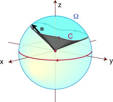
Figure 1: The geometric phase is proportional to the solid angle spanned by the Hamiltonian with respect of its degeneracy point.

The simplest, but still significant example of geometric phase, is the one obtained for a two-level system, such as a spin-1/2 particle in the presence of a magnetic field. Its Hamiltonian is given by

$$H(\theta,\phi)=\mathbf{B}(\theta,\phi)\cdot\mbox{\boldmath{$\sigma$}}=|\mathbf{B}|U(\theta,\phi)\sigma^{z}U^{\dagger}(\theta,\phi),$$ (4)

where $(\theta,\phi)$ determine the orientation of the magnetic field, $U(\theta,\phi)=e^{-i\sigma^{z}\phi/2}e^{-i\sigma^{y}\theta/2}$ is a $SU(2)$ transformation which rotates the operator $\mathbf{B}\cdot\mbox{\boldmath{$\sigma$}}$ to the $z$-direction and $\mbox{\boldmath{$\sigma$}}=(\sigma^{x},\sigma^{y},\sigma^{z})$ is the vector of Pauli’s operators, given by

$$\sigma^{x}=\left(\begin{array}[]{cc}0&1\\ 1&0\end{array}\right),\,\,\,\,\,\,\sigma^{y}=\left(\begin{array}[]{cc}0&-i\\ i&0\end{array}\right),\,\,\,\,\,\,\sigma^{z}=\left(\begin{array}[]{cc}1&0\\ 0&-1\end{array}\right).$$ (5)

With this parametrization the Hamiltonian can be represented as a vector on a sphere, centered in the point of degeneracy of the Hamiltonian ($|\mathbf{B}|=0$), as seen in Figure 1.

For $\theta=\phi=0$ we have that $U=\mbox{$1{\bf l}$}$ and the two eigenstates of the system given by $|+\rangle=(1,0)^{T}$ and $|-\rangle=(0,1)^{T}$ with corresponding eigenvalues $E_{\pm}=\pm|\mathbf{B}|/2$. Let us consider the evolution resulting when a closed path $C$ is spanned adiabatically on the sphere. Following the previous general consideration it is easy to show that the Berry connection components corresponding, e.g. to the $|+\rangle$ state, are given by

$$A_{\theta}=0,\,\,\,A_{\phi}=\frac{1}{2}\left(1-\cos\theta\right)$$ (6)

that leads to the geometric phase

$$\phi=\oint_{C}\mathbf{A}\cdot\\ dr=\frac{1}{2}\int_{\Sigma(\theta,\phi)}\!\!\!\sin{\theta}\;d\theta d\phi=\frac{\Omega}{2}.$$ (7)

The geometric phase that corresponds to the $|-\rangle$ state is given by $\gamma(C)=-\Omega/2$. Here $\Omega=\int\!\!\int_{\Sigma}sin\theta d\theta d\phi$ is the solid angle enclosed by the loop, as seen from the degeneracy point. In this expression the geometric origin of the geometric phase $\phi$ is evident. Its value depends only on the way in which these parameters are changed in relation with the degeneracy point of the Hamiltonian.

A particularly interesting case is the one in which the Hamiltonian can be casted in a real form, corresponding to $\theta=\pi/2$. In this case the phase becomes $\phi=\pi$ reproducing the sign change of the eigenstate, when it circulates a point of degeneracy ($|\mathbf{B}|=0$), in agreement with Longuet-Higgins theorem.

3 The XY model and its criticality

In order to illustrate the connection between geometric phases and critical spin systems we shall consider the concrete example of a chain of spin-1/2 particles subject to XY interactions. This is a one dimensional model with nearest neighbors spin-spin interactions, where we allow the presence of an external magnetic field oriented along the $z$-direction. The Hamiltonian is given by

$$H=-\sum_{l=-M}^{M}\left(\frac{1+\gamma}{2}\sigma^{x}_{l}\sigma^{x}_{l+1}+\frac{1-\gamma}{2}\sigma^{y}_{l}\sigma^{y}_{l+1}+\frac{\lambda}{2}\sigma^{z}_{l}\right),$$

where $\sigma^{\mu}_{l}$ are the Pauli matrices at site $l$, $\gamma$ is the x-y anisotropy parameter and $\lambda$ is the strength of the magnetic field. This model was first explicitly solved by Lieb et al. (1961) and by Katsura (1962). Since the XY model is exactly solvable and still presents a rich structure it offers a benchmark to test the properties of geometric phases in the proximity of criticalities.

In particular, we are interested in a generalization of Hamiltonian (3) obtained by applying to each spin a rotation with angle $\phi$ around the $z$-direction

$$H(\phi)=U(\phi)HU^{\dagger}(\phi)\quad\text{ with }\quad U(\phi)=\prod_{l=-M}^{M}e^{i\sigma^{z}_{l}\phi/2},$$ (8)

in the same way as we did for the single spin-1/2 particle. The family of Hamiltonians generated by varying $\phi$ is clearly isospectral and, therefore, has the same energy spectrum as the initial Hamiltonian. In addition, due to the bilinear form of the interaction term we have that $H(\phi)$ is $\pi$-periodic in $\phi$. The Hamiltonian $H(\phi)$ can be diagonalized by a standard procedure based on the Jordan-Wigner transformation and the Bogoliubov transformation (Carollo & Pachos 2005). From this procedure one can obtain the ground state, $\left|g\right\rangle$, which is given by

$$\left|g\right\rangle\!=\!\!\!\prod_{\otimes k>0}\!\!\Big{(}\!\cos{\theta_{k}\over 2}\left|0\right\rangle_{\!k}\left|0\right\rangle_{\!\!-k}\!\!-ie^{2i\phi}\sin{\theta_{k}\over 2}\left|1\right\rangle_{\!k}\left|1\right\rangle_{\!\!-k}\!\Big{)},$$ (9)

where $\left|0\right\rangle_{k}$ and $\left|1\right\rangle_{k}$ are the vacuum and single fermionic excitation of the k-th momentum mode. The angle $\theta_{k}$ is defined by $\cos\theta_{k}=\epsilon_{k}/\Lambda_{k}$ with $\epsilon_{k}=\cos{2\pi k\over N}-\lambda$ and the energy gap above the ground state is given by $\Lambda_{k}=\sqrt{\epsilon_{k}^{2}+\gamma^{2}\sin^{2}{2\pi k\over N}}$. It is remarkable that by inspection of (9) the ground state can be interpreted as the direct product of $N$ spins each one having its own orientation given by the direction $(2\phi,\theta_{k})$. As we will see in the next section this observation will make the evaluation of the ground state geometric phase a simple task. Before investigating the geometric properties of the XY model we will first consider the behavior of the spectrum as a function of the external parameters $\gamma$, $\lambda$ and $\phi$.

Let us first review the concept of quantum phase transitions. A many body system, driven by a parameter $g$, undergoes a quantum phase transition at a point $g=g_{c}$ when the energy density of the ground state at $g=g_{c}$ is non-analytic. This point is associated with a crossing or an avoiding of the energy eigenvalues. It is characterized by either a discontinuity in the first derivative of the ground state energy density (first-order phase transition) or by discontinuity or divergence in the second derivative of the ground state energy density (second-order quantum phase transition) assuming that the first derivative is continuous. In particular, the energy gap $\Delta$ between the ground and the first excited states vanishes like $\Delta\propto|g-g_{c}|^{z\nu}$ as $g$ approaches $g_{c}$ creating a point of degeneracy that we will call critical. Moreover, the non-analyticity of the energy eigenvalues is related to abrupt changes in the ground state properties. As these transitions occur at zero temperature they are driven purely by quantum fluctuations (Sachdev 2001). It can be shown that the length of the associated quantum correlations, $\xi$, diverges like $\xi^{-1}\propto|g-g_{c}|^{\nu}$ as $g$ approaches the critical point $g_{c}$. The parameters $z$ and $\nu$ are called the critical exponents and their values are universal, independent of most of the microscopic details of the system Hamiltonian.

For the case of the XY model one can identify the critical points by finding the regions where the energy gap $\Lambda_{k}$ vanishes. Indeed, there are two regions in the $\lambda$, $\gamma$ space that are critical. When $\gamma=0$ we have $\Lambda_{k}=0$ for $-1<\lambda<1$, which is a first order phase transition with an actual energy crossing and critical exponents $z=2$ and $\nu=1/2$. The other critical region is given by $\lambda=\pm 1$ where we have $\Lambda_{k}=0$ for all $\gamma$. This is a second order quantum phase transition with energy level avoiding. When $\gamma=1$ and $\lambda=\pm 1$ we obtain the Ising critical model with critical exponents $z=1$ and $\nu=1$.

Finally, let us consider the criticality behavior of the rotated Hamiltonian, $H(\phi)$. The energy gap, $\Lambda_{k}$ does not depend on the angle $\phi$, as this parameter is related to an isospectral transformation. Hence, the criticality region for the rotated Hamiltonian, $H(\phi)$, is obtained just by a rotation of the critical points of the XY Hamiltonian around the $\lambda$ axis. This is illustrated in Figure 2, where the Ising type criticality corresponds now to two planes at $\lambda=1$ and $\lambda=-1$ and the XX criticality remains along the $\lambda$ axis for $|\lambda|<1$.

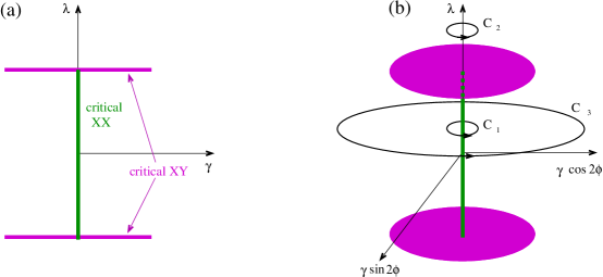
Figure 2: (a) The regions of criticality of the XY Hamiltonian are presented as a function of the parameters $\lambda$ and $\gamma$ and (b) the corresponding ones for the Hamiltonian $H(\phi)$ where $\phi$ parameterizes a rotation around the $\lambda$ axis. Possible paths for the geometric evolutions are depicted spanned by varying the parameter $\phi$.

4 Geometric phases and XY criticalities

Figure 2 depicts the critical points of the XY model. Now we are interested in spanning looping trajectories in the space comprising of the Hamiltonian parameters $\lambda$, $\gamma$ and $\phi$. The aim is to determine the geometric evolutions corresponding to these paths and relate them to the criticality regions. A special family of paths is of interest that circulates the $\lambda$ axis just by varying the $\phi$ parameter from zero to $\pi$. Indeed, these paths enclose the XX criticality only when $-1<\lambda<1$. As we shall see in the following it is possible to evaluate the corresponding geometric phases of the ground and the first excited states as a function of $\lambda$ and $\gamma$.

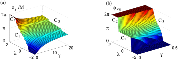
Figure 3: The geometric phase corresponding to the ground state (a) and the relative one between the ground and first excited state (b) as a function of the path parameters $\lambda$ and $\gamma$. Each point of the surface corresponds to the geometrical phase for a path that is spanned by varying $\phi$ from $0$ to $\pi$ for certain $\lambda$ and $\gamma$. The values of the geometric phase corresponding to the loops $C_{1}$, $C_{2}$ and $C_{3}$ in Figure 2 are also indicated.

Using the standard formula it is easy to show that the geometric phase of the ground state $\left|g\right\rangle$ is given by

$$\varphi_{g}=-i\int_{0}^{\pi}\left\langle g\right|\frac{\partial}{\partial\phi}\left|g\right\rangle=\sum_{k>0}\pi(1-\cos\theta_{k}).$$ (10)

This result can be understood by considering the form of $\left|g\right\rangle$, which is a tensor product of states, each lying in the two dimensional Hilbert space spanned by $\left|0\right\rangle_{k}\left|0\right\rangle_{-k}$ and $\left|1\right\rangle_{k}\left|1\right\rangle_{-k}$. For each value of $k(>0)$, the state in each of these two-dimensional Hilbert spaces can be represented as a Bloch vector with coordinates $(2\phi,\theta_{k})$. A change in the parameter $\phi$ determines a rotation of each Bloch vector about the $z$-direction. A closed circle will, therefore, produce an overall phase given by the sum of the individual phases as given in (10) and illustrated in Figure 3(a).

Of particular interest is the relative geometric phase between the first excited and ground states given by the difference of the geometric phases acquired by these two states. The first excited state is given by

$$\left|e_{k_{0}}\right\rangle=\!\!\!\left|1\right\rangle_{\!k_{0}}\left|0\right\rangle_{\!\!-k_{0}}\prod_{\otimes k>0,\,\,k\neq\pm k_{0}}\!\!\Big{(}\!\cos{\theta_{k}\over 2}\left|0\right\rangle_{\!k}\left|0\right\rangle_{\!\!-k}\!\!-ie^{2i\phi}\sin{\theta_{k}\over 2}\left|1\right\rangle_{\!k}\left|1\right\rangle_{\!\!-k}\!\Big{)},$$ (11)

with $k_{0}$ corresponding to the minimum value of the energy $\Lambda_{k}$. The behavior of this state is similar to a direct product of only $N-1$ spins oriented along $(2\phi,\theta_{k})$ where the state of the spin corresponding to momentum $k_{0}$ does not contribute any more to the geometric phase. Thus the relative geometric phase between the ground and the excited states becomes

$$\varphi_{eg}\equiv\varphi_{e}-\varphi_{g}=-\pi(1-\cos\theta_{k_{0}})$$ (12)

In the thermodynamical limit ($N\to\infty$), $\phi_{eg}$ takes the form

$$\varphi_{eg}=\left\{\begin{array}[]{cl}0,&\text{for $|\lambda|>1-\gamma^{2}$}\\ -\pi+{\pi\lambda\gamma\over\sqrt{(1-\gamma^{2})(1-\gamma^{2}-\lambda^{2})}},&\text{for $|\lambda|<1-\gamma^{2}$}\end{array}\right.$$ (13)

where the condition $|\lambda|>1-\gamma^{2}$ constrains the excited state to be completely oriented along the $z$-direction resulting in a zero geometric phase. As can be seen from Figure 3(b), the most interesting behavior of $\varphi_{eg}$ is obtained in the case of $\gamma$ small compared to $\lambda$. In this case $\varphi_{eg}$ behaves as a step function, giving either $\pi$ or $0$ phase, depending on whether $|\lambda|<1$ or $|\lambda|>1$, respectively. This behavior is precisely determined from whether the corresponding loop encloses a critical point or not and can be used as a witness of its presence. In particular, in the $|\lambda|<1-\gamma^{2}$ case the first term corresponds to a purely topological phase, while the second is a geometric contribution. Indeed, the first part gives rise to a phase which depends solely on the topological character of the trajectory traced by the $(2\phi,\theta_{k})$ coordinates. In particular if $n$ circulations are performed then the topological phase is $n\pi$, where $n$ is the winding number. The second term is geometric in nature and it can be made arbitrarily small by tuning appropriately the couplings $\lambda$ or $\gamma$. This idea is illustrated in Figure 4, where the energy surface of ground and first excited state is depicted. The point of degeneracy is the intersection of the two surfaces. This is the point where the energy density is not analytical. Consider the case of a family of loops converging to a point. In the trivial case where the limiting point does not coincide to a degeneracy, the corresponding geometric phase converges to zero. If instead, the degeneracy point is included, the geometric phase tends to a finite value (Hamma 2006).

To better understand the properties of the relative geometric phase, we focus on the region of parameters with $\gamma\ll 1$. In this case, it can be shown (Carollo & Pachos 2005) that the Hamiltonian, when restricted to its lowest energy modes, can be casted in a real form and, for $|\lambda|<1$, its eigenvalues present a conical intersection centered at $\gamma=0$.

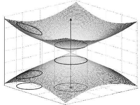
Figure 4: The conical intersection between the two lowest energy levels of the Hamiltonian as a function of its parameters. A contractible loop, i.e. a loop that can be continuously deformed to a point of the domain, produces a zero geometric phase. A non-trivial geometric phase is obtained from non-contractible loops.

It is well known that when a closed path is taken within the real domain of a Hamiltonian, a topological phase shift $\pi$ occurs only when a conical intersection is enclosed. In the present case, the conical intersection corresponds to a point of degeneracy where the XX criticality occurs and it is revealed by the topological term in the relative geometric phase $\varphi_{eg}$. It is worth noticing that the presence of a conical intersection indicates that the energy gap scales linearly with respect to the coupling $\gamma$ when approaching the degeneracy point. This implies that the critical exponents of the energy, $z$, and of the correlation length, $\nu$, satisfy the relation $z\nu=1$ which is indeed the case for the XX criticality (Sachdev 2001). In the following we shall see that geometric phases are sufficient to determine the exact values of the critical exponents and thus provide a complete characterization of the criticality behavior.

5 The general case

We shall show here that the vacuum expectation value of a hermitian operator, $O$, can be written in terms of a geometric phase. This is a rather general result that can be used to study critical models, usually probed by the behavior of vacuum expectation values of observables, just by considering geometric phases. We assume, first, that $O$ does not commute with the Hamiltonian, a requirement satisfied for the case of a non-degenerate spectrum and, second, that $O$ can transform the ground state in a cyclic fashion. The latter provides the looping trajectories of the geometric evolutions.

To show that let us extend the initial Hamiltonian, $H_{0}$, of the model in the following way

$$H(\lambda)=H_{0}+\lambda O$$ (14)

Turning to the interaction picture with respect to $O$ we obtain

$$H_{\text{int}}(\lambda)=U(\lambda t)H_{0}U^{\dagger}(\lambda t)$$ (15)

where $U(\lambda t)=\exp(-i\lambda Ot)$. From the cyclicity requirement there exists time $T$ such that the unitary rotation $U(\lambda T)$ takes the ground state $\left|\psi\right\rangle$ to itself, i.e. $U(\lambda T)\left|\psi\right\rangle=\left|\psi\right\rangle$. Hence, the desired cyclic evolution is obtained by a rotation generated by $O$. The geometric phase that result from the cyclic evolution is given by (2) and, thus, we have

$$\varphi=\lambda T\left\langle\psi\right|O\left|\psi\right\rangle$$ (16)

Hence, the expectation value of an operator that can generate circulations of the ground state is expressible with respect to a geometric phase.

One can easily verify this relation for the simple case of a spin-1/2 particle in a magnetic field. When the direction of the magnetic field is changed adiabatically and isospectrally then the state of the spin is guided in a cyclic path around the $z$-direction. The generated phase is given by $\varphi=\pi(1-\cos\theta)$, where $\theta$ is the fixed direction of the magnetic field with respect to the $z$-direction. On the other hand, one can easily evaluate that the expectation value of the operator $(1-\sigma^{z})/2$ that generates the cyclic evolution is given by $\left\langle\psi\right|(1-\sigma^{z})/2\left|\psi\right\rangle=(1-\cos\theta)/2$ which verifies relation (16) as for this example $\lambda T=2\pi$.

This connection has far reaching consequences. It is expected that intrinsic properties of the state will be reflected in the properties of the geometric phases. The latter, as they result from a physical evolution can be obtained and measured in a conceptually straightforward way. Here, we are interested in employing geometric phases to probe critical phenomena of spin systems. Indeed, from the particular example of the XY model we saw that the presence of critical points can be detected by the behavior of specific geometric evolutions and the corresponding critical exponents can be extracted. This comes as no surprise as one can choose geometric phases that correspond to the classical correlations of the system (expectation values, e.g. of $\sigma^{z}_{1}\sigma^{z}_{L}$) from where the correlation length and the critical behavior can be obtained.

Let us apply this idea to the XY model we studied earlier. There the rotations are generated by the operator $O=\sum_{l}\sigma^{z}_{l}$. Hence, the resulting geometric phase is proportional to the total magnetization

$$M_{z}=\left\langle\psi\right|\sum_{l}\sigma^{z}_{l}\left|\psi\right\rangle$$ (17)

It is well known (Sachdev 2001) that the mangetization $M_{z}$ can serve as an order parameter, from which one can derive all the critical properties of the XY model just by considering its scaling behavior. Indeed, Zhu 2006 has considered the scaling of the ground state geometric phase of the XY model from where he evaluated the Ising critical exponents. As it has been shown here this is a general property that can be applied to any critical system.

6 Physical implementation with optical lattices

This construction, apart from its theoretical interest, offers a possible experimental method to detect critical regions without the need to cross them. When a physical system is forced to go through a critical region then excited states may become populated due to the vanishing energy gap, thus undermining the identification of the system state. Hence, being able to probe the critical properties of a physical systems just by evolving it around the critical area is of much interest to experimentalists as the energy gap can be kept to a finite value.

In particular, we shall implement this model with optical lattices a system that has proven versatile in the field of quantum simulations. To this end, consider two bosonic species labelled by $\sigma=a,b$ that can be given by two hyperfine levels of an atom. Each one can be trapped by a laser field configured as a standing wave that is heavily detuned from any atomic transitions. Thus, the atom acts as a dipole in the presence of a periodic sinusoidal trapping potential that can generate one, two or three dimensional lattices. Here we will restrict to the case where the atoms in an arbitrary superposition of state $a$ and $b$ are confined in a one dimensional array by the help of two in-phase optical lattices. The tunnelling of atoms between neighboring sites is described by

$$V=-\sum_{l\sigma}(J_{\sigma}a_{l\sigma}^{\dagger}a_{(l+1)\sigma}+\text{H.c.})$$ (18)

where $a_{\sigma}$ and $a^{\dagger}_{\sigma}$ are the annihilation and creation operators of particles $\sigma$ and $J_{\sigma}$ their corresponding tunnelling coupling. When two or more atoms are present in the same site, they experience collisions given by

$$H^{(0)}=\sum_{l\sigma\sigma^{\prime}}{U_{\sigma\sigma^{\prime}}\over 2}a^{\dagger}_{l\sigma}a^{\dagger}_{l\sigma^{\prime}}a_{l\sigma^{\prime}}a_{l\sigma}$$ (19)

where $U_{\sigma\sigma^{\prime}}$ are the collisional couplings between atom species $\sigma$ and $\sigma^{\prime}$. We shall consider the limit $J\ll U$ where the system is in the Mott insulator regime with one atom per lattice site (Kastberg et al. 1995; Raithel et al. 1998). In this regime, the effective evolution is obtained by adiabatic elimination of the states with a population of two or more atoms per site, which are energetically unfavorable. Hence, to describe the Hilbert space of interest, we can employ the pseudospin basis of $|\!\!\uparrow\rangle\equiv|n_{l}^{a}=1,n_{l}^{b}=0\rangle$ and $|\!\!\downarrow\rangle\equiv|n_{l}^{a}=0,n_{l}^{b}=1\rangle$, for lattice site $l$, and the effective evolution can be expressed in terms of the corresponding Pauli (spin) operators.

It is easily verified by perturbation theory that when the tunnelling coupling of both atomic species is activated, the following exchange interaction is realized between neighboring sites (Kuklov & Svistunov 2003; Duan et al. 2003)

$$H_{1}=-\frac{J_{a}J_{b}}{U_{ab}}\sum_{l}\left(\sigma^{x}_{l}\sigma^{x}_{l+1}+\sigma^{y}_{l}\sigma^{y}_{l+1}\right).$$ (20)

In order to create an anisotropy between the $x$ and $y$ spin directions, we activate a tunnelling by means of Raman couplings (Duan et al. 2003). Application of two standing lasers $L_{1}$ and $L_{2}$, with zeros of their intensities at the lattice sites and with phase difference $\phi$, can induce tunnelling of the state $|+\rangle\equiv({e^{-i\phi/2}|a\rangle+e^{i\phi/2}|b\rangle)/\sqrt{2}}$. The resulting tunnelling term is given by $V_{c}=J_{c}\sum_{l}(c^{\dagger}_{l}c_{l+1}+\text{H.c.})$, where $c_{l}$ is the annihilation operator of $|+\rangle$ state particles. The tunnelling coupling, $J_{c}$, is given by the potential barrier of the initial optical lattice superposed by the potential reduction due to the Raman transition. The resulting evolution is dominated by an effective Hamiltonian given, up to a readily compensated Zeeman term, by

$$H_{2}=-{1\over 2}{J_{c}^{2}\over U_{ab}}\sum_{l}U(\phi)\sigma^{x}_{l}\sigma^{x}_{l+1}U^{\dagger}(\phi)$$ (21)

where $U(\phi)$ was defined in (8). Combining the rotationally invariant Heisenberg interaction $H_{1}$ with $H_{2}$ gives the rotated XY Hamiltonian described by equation (8), where the parameter $\gamma$ is given by $J_{c}^{2}/(2\epsilon U_{ab})$ and $\epsilon=(2J_{a}J_{b}+J_{c}^{2}/2)/U_{ab}$ is the overall energy scale multiplying the Hamiltonian (3). The magnetic field term $\lambda\sum_{l}\sigma^{z}_{l}$ is easily produced by a homogeneous and heavily detuned laser radiation. If the radiation has amplitude $\Omega$ and detuning $\Delta$ then the magnetic coupling is given by $\lambda=\Omega^{2}/\Delta$. Finally, the angle $\phi$ of the rotated XY Hamiltonian is given by the phase difference, $\phi$, of the lasers $L_{1}$ and $L_{2}$. Hence, the complete control of the rotated XY Hamiltonian can be obtained by the optical lattice configuration presented here and the geometric evolutions can be performed by varying the phase $\phi$ from $0$ to $\pi$.

7 Conclusions

In this article, we have presented a method that theoretically, as well as experimentally, allows for the detection of regions of criticality through the geometric phase, without the need for the system to experience quantum phase transitions. The latter is experimentally hard to realize as the adiabaticity condition breaks down at the critical point and the state of the system is no longer faithfully represented by the ground state. Alternatively, the finite energy gap $\Lambda_{k}$ that is present along the circular procedure is sufficient to adiabatically prevent unwanted transitions between the ground state and the excited ones, even in the thermodynamical limit.

The origin of the geometric phase can be ascribed to the existence of degeneracy points in the parameter space of the Hamiltonian (Hamma 2006). Hence, a criticality point can be detected by performing a looping trajectory around it and detecting whether or not a non-zero geometric phase has been generated. For the case of the XY model the topological nature of the resulting phase pinned to the value, $\varphi_{eg}\approx\pi$, is revealed by its resilience with respect to small deformations of the loop. This characteristic results from the conical intersection structure of the potential surfaces that is equivalent to having the critical exponents satisfying $z\nu=1$. In addition, the critical exponents can be evaluated by scaling arguments of the geometric phases (Zhu 2005). Hence, additional information about the critical exponents can be deduced from the topological nature and the exact value of the geometric phase. Moreover, topological phases are inherently resilient against control errors, a property that can be proved to be of a great advantage when considering many-body systems. Such a study can be theoretically performed on any system which can be analytically elaborated such as the case of the cluster Hamiltonian (Pachos & Plenio 2004), or exploited numerically when analytic solutions are not known. The generalization of these results to a wide variety of critical phenomena and their relation to the critical exponents is a promising and challenging question which deserves extensive future investigation.

References

- [1]
- [2] Aharonov, Y. & Bohm, D. 1959 Phys. Rev. 115, 485–491.
- [3]
- [4] Berry, M. B. 1984 Proc. R. Soc. Lond. A 329, 45.
- [5]
- [6] Bohm, A., Mostafazadeh, A., Koizumi, H., Niu, Q. & Zwanziger, J. 2003 The Geometric Phase in Quantum Systems, Ed. Springer.
- [7]
- [8] Carollo, A. C. M. & Pachos, J. K. 2005 Phys. Rev. Lett. 95, 157203.
- [9]
- [10] Duan, L.-M., Demler, E. & Lukin, M. D. 2003 Phys. Rev. Lett. 91, 090402.
- [11]
- [12] Hamma, A. 2006 quant-ph/0602091.
- [13]
- [14] Herzberg, G. & Longuet-Higgins, H. C. 1963 Discuss. Faraday Soc, 35, 77; Longuet-Higgins, H. C. 1975 Proc. R. Soc. London, Ser. A 344, 17.
- [15]
- [16] Johansson, N. & Sjöqvist, E. 2004 Phys. Rev. Lett. 92, 060406.
- [17]
- [18] Kastberg, A., et al. 1995 Phys. Rev. Lett. 74, 1542.
- [19]
- [20] Katsura, S. 1962 Phys. Rev. 127 1508.
- [21]
- [22] Kuklov, A. B. & Svistunov, B. V. 2003 Phys. Rev. Lett. 90, 100401.
- [23]
- [24] Lieb, E., Schultz, T. & Mattis, D. 1961 Annals of Phys. 16 407.
- [25]
- [26] Nakamura, M. & Todo, S. 2002 Phys. Rev. Lett. 89, 077204.
- [27]
- [28] Pachos, J. K. & Plenio, M. B. 2004 Phys. Rev. Lett. 93, 056402.
- [29]
- [30] Pachos, J. K. & Rico, E. 2005 Phys. Rev. A 70, 053620.
- [31]
- [32] Raithel, G., et al. 1998 Phys. Rev. Lett. 81, 3615.
- [33]
- [34] Resta, R. 1994 Rev. Mod. Phys. 66, 899.
- [35]
- [36] Ryu, S. & Hatsugai, Y. 2006 cond-mat/0601237 .
- [37]
- [38] Sachdev, S. 2001 Quantum Phase Transitions, Cambridge University Press, Cambridge, UK.
- [39]
- [40] Shapere, A. & Wilczek, F. 1989 Geometric phases in physics, World Scientific, Singapore.
- [41]
- [42] Stone, A. J. 1976 Proc. R. Soc. London, Ser. A 351, 141.
- [43]
- [44] Thouless, D. J., et al. 1982 Phys. Rev. Lett. 49, 405.
- [45]
- [46] Wen, X.-G. 2002 Quantum field theory of many-body systems, Oxford University Press.
- [47]
- [48] Zhu, S.-L. to appear in Phys. Rev. Lett, cond-mat/0511565.
- [49]