On the identification of the ground state based on occupation probabilities:
An investigation of Smith’s apparent counterexamples 

Abstract.

We study a set of truncated matrices, given by Smith [8], in connection to an identification criterion for the ground state in our proposed quantum adiabatic algorithm for Hilbert’s tenth problem. We identify the origin of the trouble for this truncated example and show that for a suitable choice of some parameter it can always be removed. We also argue that it is only an artefact of the truncation of the underlying Hilbert spaces, through showing its sensitivity to different boundary conditions available for such a truncation. It is maintained that the criterion, in general, should be applicable provided certain conditions are satisfied. We also point out that, apart from this one, other criteria serving the same identification purpose may also be available.

In a proposal of a quantum adiabatic algorithm for Hilbert’s tenth problem [5], we employ an adiabatic process with a time-dependent Hamiltonian

(1) $${\mathfrak{H}}(t) = (1-t/T)H_{I}+(t/T)H_{P}.$$

Here $t$ is time and this Hamiltonian metamorphoses from $H_{I}$ when $t=0$ to $H_{P}$ when $t=T$. The final Hamiltonian $H_{P}$ encodes the Diophantine equation in consideration, while the initial $H_{I}$ is universal and independent of the Diophantine equation, except only on its number of variables $K$. The process is captured by the Schrödinger equation

(2) $$\partial_{t}|\psi(t)\rangle = -i\mathfrak{H}(t)|\psi(t)\rangle,$$

$$|\psi(0)\rangle = |\{\alpha\}\rangle,$$

where $|\{\alpha\}\rangle$ is the ground state of the initial infinite-dimensional Hamiltonian $H_{I}$, which we choose to be

(3) $$H_{I} = \sum_{i=1}^{K}(a^{\dagger}_{i}-\alpha_{i}^{*})(a_{i}-\alpha_{i}).$$

This choice is not unique, but with it, $|\{\alpha\}\rangle$ is then the Cartesian product, of $K$ factors, of the well-known coherent states in quantum physics.

In order to identify the ground state at the final time $t=T$, we have shown in the case of 2-dimensional spaces [2] that if we could choose $\alpha$ such that $\left|\langle\psi(0)|\{n\}\rangle\right|^{2}<0.5$, for all $|\{n\}\rangle$ which are the Fock states and also the eigenstates of $H_{P}$, then

(4) $${\mbox{\rm If }}\left|\langle\psi(T)|\{n^{(0)}\}\rangle\right|^{2}>\frac{1}{2} \Rightarrow |\{n^{(0)}\}\rangle\;{\mbox{\rm is the ground state of }}H_{P},$$

assuming such a ground state is non-degenerate, and provided an extra condition has to be satisfied, for all $0<t<T$, namely

(5) $$\langle e(t)|H_{P}-H_{I}|g(t)\rangle \not= 0,$$

where $|g(t)\rangle$ and $|e(t)\rangle$ are, respectively, the instantaneous ground state and the first excited state of $\mathfrak{H}(t)$ at the time $t$. The violation of that condition at some $t_{0}$ is equivalent to

(6) Both $$\langle e(t_{0})|H_{P}|g(t_{0})\rangle=0,$$

(7) And $$\langle e(t_{0})|H_{I}|g(t_{0})\rangle=0.$$

In two dimensions this criterion for the ground-state identification can easily and always be satisfied for $H_{I}$ and $H_{P}$ noncommutting, which is automatic for our choice of $H_{I}$. For higher dimensions, the non-commutativity of the Hamiltonians is no longer a sufficient condition for (5). And we need make sure that the condition (5) is observed.

Recently, Smith has claimed to have three counterexamples [8] against the criterion (4) above. Of the three provided, actually there is only one that is relevant and fits the form of our time-dependent Hamiltonian (1) in the case of one variable, but truncated to five dimensions and with the diagonal term $(1-|\alpha|^{2}){\bf 1}$ added to (3),

(18) $$H_{I}^{S}=\left(\begin{array}[]{ccccc}1&-\alpha^{*}&0&0&0\\ -\alpha&2&-\alpha^{*}\sqrt{2}&0&0\\ 0&-\alpha\sqrt{2}&3&-\alpha^{*}\sqrt{3}&0\\ 0&0&-\alpha\sqrt{3}&4&-2\alpha^{*}\\ 0&0&0&-2\alpha&5\end{array}\right); H_{P}^{S}=\left(\begin{array}[]{ccccc}2&0&0&0&0\\ 0&4&0&0&0\\ 0&0&5&0&0\\ 0&0&0&3&0\\ 0&0&0&0&1\end{array}\right).$$

Smith has chosen the particular values $\alpha=1$ and $T=13.3444$. In this note we shall only investigate this example; other criticisms by Smith in [8] also overlap with others’, our replies to which have been given in [5].

Indeed, when we solve the Schrödinger equation (On the identification of the ground state based on occupation probabilities: An investigation of Smith’s apparent counterexamples ), starting with the exact ground state of $H_{I}^{S}$, we obtain at time $t=0$ no Fock-state occupation probabilities is more than 0.5, but at $t=T$, the first excited Fock state has a probability of 0.999323 – apparently contradicting the criterion (4). We have depicted the occupation probabilities of the instantaneous ground and first excited states as functions of time in Fig. 1. At first, the ground-state occupation is close to one, as it should be because we start the system in the initial ground state. Then, suddenly at around $t\approx 10$ this probability plummets to zero, accompanying by a stellar rise of that of the first excited state.

Figure 1. The occupation probabilities of the instantaneous ground state (unfilled boxes) and first excited state (triangles) as functions of time, for $\alpha=1$. The excited-state probability rises suddenly from near zero to close to one around $t\approx 10$, which corresponds to the near miss of these two energy levels as shown in Fig. 2. The filled circles are for the instantaneous ground-state occupation for $\alpha=3$, which shows no sudden change. See text for further explanation.

A closer inspection of spectral flow (the flow of eigenvalues of $\mathfrak{H}(t)$ as functions of time) reveals a singular behaviour of the flow also around $t\approx 10$, namely, that of an avoided crossing of the instantaneous ground and first excited state as shown in Figs. 2 and 3.

Figure 2. The spectral flow for $\alpha=1$. The apparent crossing of the lowest two energy levels just after $t\approx 10$ is actually an avoided crossing as shown in Fig. 3.

Figure 3. An avoided crossing for the lowest two energy levels for $\alpha=1$. Note the large variations in the first derivatives of the branches.

As a matter of fact, all these anomalous behaviours are caused by the violation of the condition (5), or equivalently, by the realisation of (6) and (7), as shown by the simultaneous vanishing of the three matrix elements, see Fig. 4, around (but a bit earlier than) the time of the anomalous transfer of probability from the ground state to the first excited state.

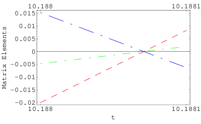
Figure 4. The sudden change in occupation probabilities in Fig. 1 at certain time $t_{0}$ is due to the simultaneous vanishing, at exactly the same time (and a bit earlier than $t_{0}$), of the three different matrix elements in (5), (6) and (7) – respectively corresponding to the (red) dash line, the (green) dash-dot line, and the (blue) long dash-dot line.

Appropriately large values for $\alpha$

Surely, for that value of $\alpha=1$ one could increase $T$ and eventually will have an arbitrarily high occupation probability of the final ground state, as guaranteed by the quantum adiabatic theorem. However, for the present value of $T=13.3444$ we can avoid the violation of (5), and thus restore the criterion (4), by widening the gap between the instantaneous ground and first excited states. This can be achieved by choosing an appropriately large value for the parameter $\alpha$. In Fig. 5 we plot the occupation probabilities of the instantaneous ground and first excited states as functions of $\alpha$. It is seen that as long as $\alpha>2$ our identification criterion (4) is again valid.

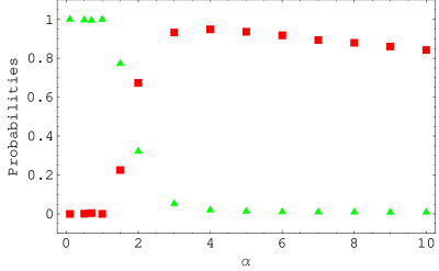
Figure 5. The final occupation probabilities for the ground state (red boxes) and first excited state (green triangles) at $T=13.3444$ for different values of $\alpha$’s. As expected, the true ground state dominates for larger $\alpha$.

We present further results for $\alpha=3$, as an example, in Figs. 6, 7 and 8. None of those shows any anomalous behaviour. (We also plot the ground state occupation for $\alpha=3$ (filled black circles) in Fig. 1 for comparison with the case $\alpha=1$.)

Figure 6. The occupation probability of the instantaneous ground state as a function of time, for $T=13.3444$ but with $\alpha=3$. (Note that the vertical scale does not go down to zero.)

Figure 7. The spectral flow shows no anomalous behaviour for $\alpha=3$.

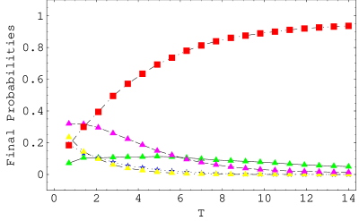
Figure 8. The probabilities, for $\alpha=3$, for different Fock states as functions of the final time $T$. There is only one state that has a probability eventually rising above 0.5 (red boxes) and that is the true ground state of $H_{P}^{S}$, namely $|4\rangle$.

We have provided some arguments in [5] to indicate that the condition (5) can always be obtained for sufficiently large values of $|\alpha|$. The larger this value is, the more dominant role $H_{I}$ has in $\mathfrak{H}(t)$, such that the lowest branch of the spectral flow (that is, the branch of the ground state) would be straightened out as the case in Fig. 7, and any avoided crossing as the one in Figs. 2 and 3 could not be formed.

How could one estimate such a value for $|\alpha|$? One possible procedure is:
$\bullet$ We firstly choose a value for $\alpha$ and use the criterion (4) to obtain a candidate state, say $|m\rangle$.
$\bullet$ Then the diagonal term $\langle m|\mathfrak{H}(t)|m\rangle$ is of the form

(19) $$(1-t/T)(m+|\alpha|^{2})+(t/T)\langle m|H_{P}|m\rangle.$$

If we choose $\alpha$ such that the first term in (19) dominates over the second term, for some $t$ close to $T$, then $H_{I}$ would dominates over $H_{P}$ for this state and at this time. As a result, no avoided crossing (which is due to the influence of $H_{P}$) could be formed at this late $t$, and thus could never be formed. A repeat of the adiabatic process and another application of the criterion (4) would then reveal if the candidate $|m\rangle$ is the true ground state. Otherwise, a different candidate would be obtained and we could repeat the whole procedure of choosing $\alpha$ again.

Sensitivity with different boundary conditions for the truncation

In general, we suspect that the possibility of the violation of (5) is an artefact of the truncation of the Fock space since it is extremely sensitive to the truncation and its associated boundary conditions. Note also that any truncation would distort the spacings between the eigenvalues of $H_{I}$, severely away from unity particularly near the truncation. In Smith’s truncation to five dimensions, for example, the four spacings between the eigenvalues of $H_{I}^{S}$ are 1.11927, 1.40986, 1.84784, and 2.54043, respectively from the lowest to the highest eigenvalues, which are $(0.0114457,1.13072,2.54058,4.38841,6.92885)$. That is, the spacing between the fourth and fifth eigenvalues near the truncation is 2.54043, which should have been one. This and the fact that the ground state of $H_{P}^{S}$ happens to be right at the truncation, $|n\rangle=|5\rangle$, make the problem very sensitive to boundary effects.

However, the addition of extra states or the imposition of (anti)-periodic boundary conditions on the truncated spaces may remove the violation of (5), as shown below.

Figure 9. The spectral flow for $\alpha=1$, with periodic condition for the truncated Fock space.

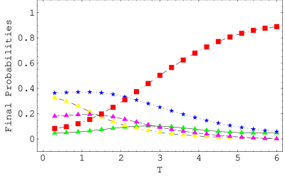
Figure 10. The final occupation probabilities for different Fock states at the final time $T$ for $\alpha=1$ but with periodic condition for the truncated Fock space. The boxes represent the true final ground state $|4\rangle$.

Figure 11. The spectral flow for $\alpha=1$, with anti-periodic condition for the truncated Fock space.

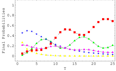
Figure 12. The final occupation probabilities for different Fock states at the final time $T$ for $\alpha=1$ but with anti-periodic condition for the truncated Fock space. The boxes represent the true final ground state $|4\rangle$.

In obtaining the truncated matrices (18), Smith has implicitly imposed the boundary condition

(20) $$a^{\dagger}\;|4\rangle=0; a|0\rangle=0,$$

on the underlying truncated Fock space. However, other boundary conditions can also be imposed on an equal footing, for example,

(21) $$a^{\dagger}\;|4\rangle=\pm\sqrt{5}\;|0\rangle; a\;|0\rangle=\pm\sqrt{5}\;|4\rangle,$$

where the plus (minus) sign corresponds to periodic (anti-periodic) boundary condition on a Fock space having only five vectors, $\{|0\rangle,|1\rangle,|2\rangle,|3\rangle,|4\rangle\}$. With these new (anti)-periodic boundary conditions, we would have

(27) $$H_{I}^{S} \to \left(\begin{array}[]{ccccc}6&-\alpha^{*}&0&0&\pm\alpha^{*}\sqrt{5}\\ -\alpha&2&-\alpha^{*}\sqrt{2}&0&0\\ 0&-\alpha\sqrt{2}&3&-\alpha^{*}\sqrt{3}&0\\ 0&0&-\alpha\sqrt{3}&4&-2\alpha^{*}\\ \pm\alpha\sqrt{5}&0&0&-2\alpha&5\end{array}\right);$$

with $a^{\dagger}a|0\rangle=5|0\rangle$, while assuming that $H_{P}^{S}$ maintains the same form. Figs. 9, 10, 11 and 12 show the non-anomalous and drastically different behaviour, as compared to (18), for the same parameters $\alpha=1$ and $T=13.3444$.

Based on such sensitivity and some other evidence, we suspect that a violation of (5) or, equivalently, a realisation of (6) and (7) could not be attained either for very large or an infinite number of dimensions, or for more than one variable. It is perhaps appropriate to mention here that all the numerical simulations presented in [5] have been obtained not with truncations with rigid boundary as the cases Smith has considered but with movable boundaries where more Fock states are included when and if necessary. Results from further analytic investigations for an infinite number of dimensions would be reported elsewhere when they become available.

We should note further that (4) may not be the only means which can be used to identify the final ground state. A more general one, as discussed in [1, 3], could be a matching of the statistics of the measurement outcomes of a physical quantum adiabatic process (in a space of presumably infinite dimensions) with those of a numerical simulation of the process with a necessarily truncated space. As the size of the truncation is enlarged, the true final ground state would eventually be included in such a truncated Fock space. From then on, further enlargement of the truncated Fock space only serves to improve the precision of the statistics comparison. (This is another manifestation of the finitely refutable nature of our problem, as mentioned in [5].)

Finally, we also would like to point out that in addition to the physical process discussed here, which is governed by the linear Schrödinger equation, we can also map Hilbert’s tenth problem into a class of non-linear differential equations [4, 6], that is readily available to pure mathematical investigation.

References

- [1] T.D. Kieu. Computing the non-computable. Contemporary Physics, 44:51–77, 2003.
- [2] T.D. Kieu. Quantum adiabatic algorithm for Hilbert’s tenth problem: I. The algorithm. ArXiv:quant-ph/0310052, 2003.
- [3] T.D. Kieu. Quantum algorithms for Hilbert’s tenth problem. Int. J. Theor. Phys., 42:1451–1468, 2003.
- [4] T.D. Kieu. A reformulation of Hilbert’s tenth problem through quantum mechanics. Proc. Roy. Soc., A 460:1535–1545, 2004.
- [5] T.D. Kieu. Hypercomputability of quantum adiabatic processes: Fact versus prejudices. ArXiv:quant-ph/0504101, 2005.
- [6] T.D. Kieu. Mathematical computability questions for some classes of linear and non-linear differential equations originated from Hilbert’s tenth problem. arXiv:math.GM/0507109, 2005.
- [7] T.D. Kieu. A mathematical proof for a ground-state identification criterion. arXiv:quant-ph/0602146, 2006.
- [8] Warren D. Smith. Three counterexamples refuting kieu’s plan for “quantum adiabatic hypercomputation”; and some uncomputable quantum mechanical tasks. http://math.temple.edu/w̃ds/homepage/works.html, #85, 2005. To appear in the Journal of the Association for Computing Machinery.