Polarization ququarts

Abstract

We discuss the concept of polarization states of four-dimensional quantum systems based on frequency non-degenerate biphoton field. Several quantum tomography protocols were developed and implemented for measurement of an arbitrary state of ququart. A simple method that does not rely on interferometric technique is used to generate and measure the sequence of states that can be used for quantum communication purposes.

I Introduction

Recently multi-dimensional quantum systems (quantum dits, or qudits) attract much attention in context of quantum information and communication. It is partly caused by fundamental aspects of quantum theory since usage of qudits allows one to violate Bell-type inequalities strongly than with two dimensional systems (qubits) quBell . Much interest in qudits also comes from the application point, especially from applied quantum key distribution. Multilevel systems are proved to be more robust against noise in the transmission channel, although measurement and preparation procedures of such systems seem to be much more technically complicated than in the case of qubits. Different aspects of the security of qudits-based protocols have been analysed QKD_Security including those related to the reduced set of bases Tittel . Lately a proof-of-principal realization of a QKD protocol with qudits Walborn:05 and with entangled qutrits ($D=3$, where $D$ is dimensionality of the Hilbert space) QKD_Zeilinger:05 have been demonstrated. For the last several years elegant experiments were performed where different kinds of optical qudits were introduced. Most of them are based on states of light emitted via spontaneous parametric down-conversion (SPDC). There are qudits obtained using spatial degrees of freedom: with either single photons Walborn:05 or twin photons Howell:05 ; orbital angular momentum of photons OAM ; time-bin tecnique timebin ; multi-armed interferometers Thew:04 ; postselection of polarization qutrits from four-photon states antia:01 , and polarization states of single-mode biphotons ourPRL:04 .

It seems that among manifold manners of qudits preparation only the method based on polarization states of single-mode biphotons admits preparation of any qutrit state (pure or mixed) on demand within one set-up and guarantees complete control over the state with high accuracy ourPRL:04 ; ourPRA:04 . However, this method does not allow to create entangled qutrits. Another limitation of polarization qutrits relates to the fundamental lock for their basic states transformations using SU(2) optical elements, like retardation plates, rotators etc. Meanwhile it is these transformations that would be extremely useful for quantum communication purposes.

In this paper we present the results of experimental preparation and measurement carried out with polarization based ququarts or quantum systems with dimensionality $D=4$. The paper is organized as follows. In Sec.II we discuss the main properties of ququarts based on the polarization state of two-photon (biphoton) field. Such operational notions as coherence matrix, polarization degree are introduced. The criterium of separability for qubits forming ququarts is discussed as well. Sec.III is devoted to different experimental implementations of biphoton-ququarts preparation and their measurement. In Sec.IV we consider a specific set of ququarts which can be used in practice for quantum key distribution.

II Polarization ququarts and their properties

II.1 Polarization states of biphoton field

Biphoton field generated via spontaneous parametric down-conversion process is represented by a coherent mixture of two-photon Fock states and the vacuum state klbook :

$$\Psi=|{vac}\rangle+\frac{1}{2}\sum\limits_{\vec{k_{i}}\vec{k_{s}}}{F_{\vec{k_{i}},\vec{k_{s}}}|{1_{\vec{k_{i}}},1_{\vec{k_{s}}}}\rangle},$$ (1)

where $|{1_{\vec{k_{i}}},1_{\vec{k_{s}}}}\rangle$ denotes the state with one (idler) photon in the mode $\vec{k_{i}}$ and one (signal) photon in the mode $\vec{k_{s}}$. Since squared modulus of the coefficient $F_{\vec{k_{i}},\vec{k_{s}}}$ gives probability to register two photons in modes $\vec{k_{i}}$ and $\vec{k_{s}}$ it is called the biphoton amplitude  kllaser . The pure polarization state of down-converted light field, which is often refered as two-photon field (or biphotons), can be written as follows:

$$|\Psi\rangle=c_{1}|2_{H},0_{V}\rangle+c_{2}|1_{H},1_{V}\rangle+c_{3}|1_{V},1_{H}\rangle+c_{4}|0_{H},2_{V}\rangle.$$ (2)

Here $c_{i}=|c_{i}|e^{i\phi_{i}}$, $\sum\limits_{i=1}^{4}{|{c_{i}}|^{2}=1}$ are complex probability amplitudes. The first ($n$) and second ($m$) place in kets corresponds to number of distinct photons with definite (either horizontal $H$ or vertical $V$) polarization, with total photon number $m+n=2$. If down converted photons have equal frequency and momentum, then a ququart state (2) converts to a qutrit state, i.e. middle terms in (2) become indistinguishable: $\vec{k}_{s}\approx\vec{k}_{i}$, $\omega_{s}\approx\omega_{i}$ and $\omega_{s}+\omega_{i}=\omega_{p}$, where $\omega_{p}$ is the laser pump frequency. In this case any arbitrary pure polarization state of biphoton field can be expressed in terms of three complex amplitudes $c_{1}^{\prime},c_{2}^{\prime},$ and $c_{3}^{\prime}$:

$$|c^{\prime}\rangle=c_{1}^{\prime}|{2,0}\rangle+c_{2}^{\prime}|{1,1}\rangle+c_{3}^{\prime}|{0,2}\rangle,$$ (3)

with $c_{i}^{\prime}=|{c_{i}^{\prime}}|\exp\{{i\varphi_{i}}\}$, $\sum\limits_{i=1}^{3}{|{c_{i}^{\prime}}|^{2}=1}$. The vector $|c^{\prime}\rangle=({c_{1}^{\prime},c_{2}^{\prime},c_{3}^{\prime}})$ represents a three-state system or a qutrit. Figure 1 presents the photograph picture of two dimensional SPDC spectrum taken in coordinates wavelength-angle. By convention the left-and-upper side in respect with doubled pump wavelength belongs to ”signal” range whereas the right-and-down side belongs to ”idler” one. The dashed lines limit the central part of the spectrum which corresponds to the frequency degenerate and collinear regime when photons forming the biphoton have approximately the same wavelengths and propagate along the pump. To select this part pinholes and/or narrow-band filters are typically used. It is that part of biphoton spectrum, that contributes to qutrits.

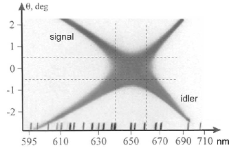
Figure 1: Photograph of lithium iodate ($LiIO_{3}$) frequency-angular spectrum taken with helium cadmium laser operated at 325nm. Angle between crystal optical axis and laser pump is $59.22^{\circ}$. Dashed lines select the part of the spectrum (frequency degenerate, collinear regime of SPDC) contributed to biphotons-qutrits. Vertical lines at the bottom belong to the spectrum of neon which serves as a frequency reference.

In order to distinguish between middle terms in (2) one must induce the distinguishability between down converted photons either in frequency, momentum or detection time. In experiments described in this paper we chose collinear non-degenerate regime of SPDC so twin photons that form a biphoton were having different frequencies and propagate along the same direction. The appropriate two-dimensional spectrum is shown in Figure 2. To take this spectrum it is enough to tilt the crystal by a small angle with respect to the orientation that is used for degenerate regime. Two dashed rectangles indicate the angular-frequency ranges of spectrum contributing to ququarts.

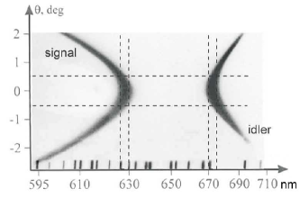
Figure 2: Non-degenerate regime of SPDC. Angle between crystal optical axis and laser pump is $58.97^{\circ}$. Dashed lines select the part of the spectrum contributed to ququarts.

The state (2) can be thus rewritten in the form:

$$|\Psi\rangle=c_{1}|H_{1},H_{2}\rangle+c_{2}|H_{1},V_{2}\rangle+c_{3}|V_{1},H_{2}\rangle+c_{4}|V_{1},V_{2}\rangle.$$ (4)

Here $|H_{{1(2)}}\rangle\equiv a_{1(2)}^{\dagger}|vac\rangle$, $|V_{{1(2)}}\rangle\equiv b_{1(2)}^{\dagger}|vac\rangle$, where $a_{1(2)}^{\dagger}$, $b_{1(2)}^{\dagger}$ are the creation operators of down-converted photons with central wavelength $\lambda_{1}$($\lambda_{2}$) in horizontal and vertical polarization mode. The alternative way to represent a ququart might be by introducing distinguishability between spatial modes while keeping the same central wavelengths of photons: $\vec{k}_{s}\neq\vec{k}_{i}$, $\omega_{s}\approx\omega_{i}$. The detailed description of polarization properties of such a state of two qubits has been done by James and co-authors Kwiat:01 . The case of ququart with two frequency modes attracts much attention because for some class of the tasks it is convenient to operate with states in single spatial mode.

II.2 Is ququart a separable or entangled state of two qubits?

Generally, the state (4) can not be written as a direct product of polarization states of two photons:

$$|\Psi_{1}\rangle\otimes|\Psi_{2}\rangle=(p_{1}|H_{1}\rangle+q_{1}|V_{1}\rangle)\otimes(p_{2}|H_{2}\rangle+q_{2}|V_{2}\rangle)$$ (5)

That is why it is useful to write down the condition when (4) becomes a separable state. The reduced density matrix of the subsystem (second photon) can be found by tracing the joint state over all states of the first photon:

$$\rho_{2}=Sp_{1}(|\Psi\rangle\langle\Psi|)=\left({{\begin{array}[]{*{20}c}{|c_{1}|^{2}+|c_{3}|^{2}\hfill}&{{c_{1}c_{2}^{*}}+{c_{3}c_{4}^{*}\hfill}}\\ {{c_{2}c_{1}^{*}}+{c_{4}c_{3}^{*}\hfill}}&{|c_{2}|^{2}+|c_{4}|^{2}\hfill}\\ \end{array}}}\right).$$ (6)

It is straightforward to show that the eigenvalues of (6) take the meanings $\lambda_{1,2}=0,1$ and entropy of each subsystem drops to zero iff

$$c_{1}c_{1}^{*}c_{4}c_{4}^{*}+c_{3}c_{3}^{*}c_{2}c_{2}^{*}-c_{2}c_{1}^{*}c_{3}c_{4}^{*}-c_{4}c_{3}^{*}c_{1}c_{2}^{*}=\\ |c_{1}c_{4}-c_{2}c_{3}|^{2}=0.$$ (7)

Thus if $c_{1}c_{4}=c_{2}c_{3}$ holds, the state (4) reduces to factorized one with definite states of each qubit $|\Psi_{1}\rangle$, $|\Psi_{2}\rangle$ and vice versa. In other words (7) plays the role of criterium for biphoton-based ququart to be a separable state of a couple of polarization qubits belonging to two different modes. Sub-indexes in (4) designate either frequency or spatial modes.

As examples of different ququarts we refer to the product states that might be generated from a single non-linear crystal via SPDC:

$${{\begin{array}[]{*{20}c}typeI:\hfill&|H_{1}H_{2}\rangle=\left({{\begin{array}[]{*{20}c}{1\hfill}\\ {0\hfill}\\ {0\hfill}\\ {0\hfill}\\ \end{array}}}\right),\hfill&|V_{1}V_{2}\rangle=\left({{\begin{array}[]{*{20}c}{0\hfill}\\ {0\hfill}\\ {0\hfill}\\ {1\hfill}\\ \end{array}}}\right),\hfill\\ typeII:\hfill&|V_{1}H_{2}\rangle=\left({{\begin{array}[]{*{20}c}{0\hfill}\\ {0\hfill}\\ {1\hfill}\\ {0\hfill}\\ \end{array}}}\right),\hfill&|H_{1}V_{2}\rangle=\left({{\begin{array}[]{*{20}c}{0\hfill}\\ {1\hfill}\\ {0\hfill}\\ {0\hfill}\\ \end{array}}}\right).\hfill\\ \end{array}}}$$ (8)

and maximally entangled Bell-states:

$$|\Psi^{\pm}\rangle=\left({{\begin{array}[]{*{20}c}{0\hfill}\\ {\frac{1}{\surd\bar{2}}\hfill}\\ {\pm\frac{1}{\surd\bar{2}}\hfill}\\ {0\hfill}\\ \end{array}}}\right),\quad|\Phi^{\pm}\rangle=\left({{\begin{array}[]{*{20}c}{\frac{1}{\surd\bar{2}}\hfill}\\ {0\hfill}\\ {0\hfill}\\ {\pm\frac{1}{\surd\bar{2}}\hfill}\\ \end{array}}}\right),$$ (9)

At the end of this section we would like to mention that biphoton-ququart is not supposed to be mapped on Poincaré sphere as a pair of points like it occurs for biphoton-qutrits ortogonality ; burjetp . Indeed it is not because the state (4) can not be factorized in the general case. However, if (7) holds the sub-set of separable qubit states admits its visual representation on Poincaré sphere.

II.3 Second order of the field: Stokes parameters

Polarization properties of a pure state (4) can be described by Stokes parameters which are the mean values of Stokes operators averaged over the state (4). Although the description of light polarization can be introduced only for the quasimonochromatic plane waves, it is possible to use $P$-quasispin formalizm karasev to describe the polarization of arbitrary quantum beams with $n$ modes, frequency or spatial. For two-frequency and single-spatial mode field, the Stokes parameters will contain time and frequency dependent terms $exp(i(\omega_{j}-\omega_{k})t)$ that describe ”beats” of frequency modes and have no connection with light polarization. However, these terms vanish if one considers the finite detection time that allows to classically average these ”beatings”. So in the case of two frequencies, the Stokes operators are given by the sum of corresponding operators in two modes

$$\begin{array}[]{cc}\langle S_{0}\rangle=\langle a_{1}^{\dagger}a_{1}+a_{2}^{\dagger}a_{2}+b_{1}^{\dagger}b_{1}+b_{2}^{\dagger}b_{2}\rangle\equiv&\\ \langle S_{0}^{(1)}\rangle+\langle S_{0}^{(2)}\rangle=2;&\\ \langle S_{1}\rangle=\langle a_{1}^{\dagger}a_{1}+a_{2}^{\dagger}a_{2}-b_{1}^{\dagger}b_{1}-b_{2}^{\dagger}b_{2}\rangle\equiv&\\ \langle S_{1}^{(1)}\rangle+\langle S_{1}^{(2)}\rangle=2(|c_{1}|^{2}-|c_{4}|^{2});&\\ \langle S_{2}\rangle=\langle a_{1}^{\dagger}b_{1}+a_{2}^{\dagger}b_{2}+b_{1}^{\dagger}a_{1}+b_{2}^{\dagger}a_{2}\rangle\equiv&\\ \langle S_{2}^{(1)}\rangle+\langle S_{2}^{(2)}\rangle=\\ 2Re(c_{1}^{\star}(c_{2}+c_{3})+c_{4}(c_{2}^{\star}+c_{3}^{\star}));&\\ \langle S_{3}\rangle=\langle a_{1}^{\dagger}b_{1}+a_{2}^{\dagger}b_{2}-b_{1}^{\dagger}a_{1}-b_{2}^{\dagger}a_{2}\rangle\equiv&\\ \langle S_{3}^{(1)}\rangle+\langle S_{3}^{(2)}\rangle=&\\ 2Im(c_{1}^{\star}(c_{2}+c_{3})+c_{4}(c_{2}^{\star}+c_{3}^{\star})).\end{array}$$ (10)

The same definition applies to the second wavelength $\lambda_{2}$ and we take into account that these operators do not commute for different frequency modes.

II.4 Fourth order of the field: Coherence matrix

Polarization properties of biphoton-ququarts are determined completely by the analogue of the coherence matrix. It is a matrix consisting of ten fourth-order moments of the electromagnetic field. An ordered set of such moments can be obtained using the direct product of $2\times{2}$-coherence matrixes for both polarization qubits forming biphoton:

$$K_{4}\equiv(K_{2})_{1}\otimes(K_{2})_{2}=\left({{\begin{array}[]{*{20}c}A\hfill&E\hfill&F\hfill&G\hfill\\ {E^{*}\hfill}&B\hfill&I\hfill&K\hfill\\ {F^{*}\hfill}&{I^{*}\hfill}&C\hfill&L\hfill\\ {G^{*}\hfill}&{K^{*}\hfill}&{L^{*}\hfill}&D\hfill\\ \end{array}}}\right),$$ (11)

where $(K_{2})_{1,2}$ are $2\times{2}$-coherence matrixes for single photons with different frequencies marked with indexes $j=1,2$:

$$(K_{2})_{j}\equiv\left({{\begin{array}[]{*{20}c}\langle a_{j}^{\dagger}a_{j}\rangle\hfill&\langle a_{j}^{\dagger}b_{j}\rangle\hfill\\ \langle a_{j}b_{j}^{\dagger}\rangle\hfill&\langle b_{j}^{\dagger}b_{j}\rangle\hfill\\ \end{array}}}\right),$$ (12)

The diagonal elements of (11) are formed by real moments, which characterize the intensity correlation in two polarization modes $H$ and $V$:

$${{\begin{array}[]{*{20}c}A\equiv\langle a_{1}^{\dagger}a_{2}^{\dagger}a_{1}a_{2}\rangle=|{c_{1}}|^{2},\quad B\equiv\langle a_{1}^{\dagger}b_{2}^{\dagger}a_{1}b_{2}\rangle=|{c_{2}}|^{2},\hfill&\\ C\equiv\langle b_{1}^{\dagger}a_{2}^{\dagger}b_{1}a_{2}\rangle=|{c_{3}}|^{2},\quad D\equiv\langle b_{1}^{\dagger}b_{2}^{\dagger}b_{1}b_{2}\rangle=|{c_{4}}|^{2}.\hfill&\\ \end{array}}}$$ (13)

Nondiagonal moments are complex:

$${{\begin{array}[]{*{20}c}E\equiv\langle a_{1}^{\dagger}a_{2}^{\dagger}a_{1}b_{2}\rangle=c_{1}^{*}c_{2},\quad F\equiv\langle a_{1}^{\dagger}a_{2}^{\dagger}b_{1}a_{2}\rangle=c_{1}^{*}c_{3},\hfill&\\ G\equiv\langle a_{1}^{\dagger}a_{2}^{\dagger}b_{1}b_{2}\rangle=c_{1}^{*}c_{4},\quad I\equiv\langle a_{1}^{\dagger}b_{2}^{\dagger}b_{1}a_{2}\rangle=c_{2}^{*}c_{3},\hfill&\\ K\equiv\langle a_{1}^{\dagger}b_{2}^{\dagger}b_{1}b_{2}\rangle=c_{2}^{*}c_{4},\quad L\equiv\langle b_{1}^{\dagger}a_{2}^{\dagger}b_{1}b_{2}\rangle=c_{3}^{*}c_{4}.\hfill&\\ \end{array}}}$$ (14)

The averaging in (13, 14) is taken over the state (4). The polarization (reduced) density matrix of ququart coincides with coherency matrix $K_{4}$.

II.5 Polarization degree and transformations of ququarts

The polarization degree is given by

$$P={\frac{\sqrt{\sum\limits_{k=1}^{3}{\langle S_{k}\rangle}^{2}}}{\langle S_{0}\rangle}}={\frac{\sqrt{\sum\limits_{k=1}^{3}{\langle S_{k}^{(1)}+S_{k}^{(2)}\rangle}^{2}}}{\langle S_{0}^{(1)}+S_{0}^{(2)}\rangle}}.$$ (15)

This definition of polarization degree is just generalization of the commonly used classical one. It differs from the definition suggested in gunnar , where it serves as a witness of the state purity. In the case of polarization-based qutrit states ourPRL:04 ; ourPRA:04 , the polarization degree is

$$P_{3}=\sqrt{|c_{1}^{\prime}|^{2}-|c_{3}^{\prime}|^{2}+2|{c_{1}^{\prime\ast}c_{2}^{\prime}+c_{2}^{\prime\ast}c_{3}^{\prime}}|^{2}}$$ (16)

with $c_{1}^{\prime}=c_{1},\sqrt{2}c_{2}^{\prime}=c_{2}=c_{3},c_{3}^{\prime}=c_{4}$. This quantity was invariant under unitary polarization transformations, which is reasonably straightforward dnk:97 . Indeed it was impossible to prepare all demanded pure states that can be used, for example, in QKD protocols, unless one uses interferometric schemes with several nonlinear crystals ourPRL:04 , or introduces losses. In particular, there is no way to transform the basic qutrit state $|\Psi_{4}^{\prime}\rangle=|V,V\rangle$ with $P$ = 1 into orthogonal state $|\Psi_{2}^{\prime}\rangle=|H,V\rangle$ with $P$ = 0 using retardation plates polardegree . However, in the case of polarization ququarts, this quantity is no longer invariant. Indeed the polarization degree (15) can be rewritten as

$$P_{4}={\frac{\sqrt{\sum\limits_{j=1}^{2}(Tr^{2}(K_{2})_{j}-2det(K_{2})_{j})+2\sum\limits_{k=1}^{3}\langle S_{k}^{(1)}S_{k}^{(2)}\rangle}}{\sum\limits_{j=1}^{2}Tr(K_{2})_{j}}}.$$ (17)

In (17) we used trivial links between coherence matrices and Stokes parameters MandelWolf .

The expression in the round brackets is invariant under unitary transformations as well as the denominator. The second term under the square root in numerator can be expanded in terms of fourth-order moments:

$$\sum\limits_{k=1}^{3}\langle S_{k}^{(1)}S_{k}^{(2)}\rangle=\{TrK_{4}-2(ReI+B+C)\}.$$ (18)

Since unitary transformations keep number of photons, then $TrK_{4}$ is invariant. At the same time it is easy to prove that combination of moments $ReI+B+C$ is not an invariant, so the whole expression (17) changes under SU(2) transformations. As a consequence, the polarization degree changes by applying local unitary transformations in each frequency mode. This can be achieved by using dichroic polarization transformers, which act separately on the photons with different frequencies. For example, to transform the state

$$|\Psi_{4}\rangle=|V_{\lambda_{1}},V_{\lambda_{2}}\rangle\Rightarrow|\Psi_{2}\rangle=|H_{\lambda_{1}},V_{\lambda_{2}}\rangle,$$ (19)

one needs to use the retardation plate which serves as a half wave plate at $\lambda_{1}$ and as a wave plate at $\lambda_{2}$.For the general case when ququart is not a product state of two qubits the transformation matrix $\hat{G}$:

$$|\Psi\rangle^{out}=\hat{G}|\Psi\rangle^{in}$$ (20)

can be found simply by making use of the Heizenberg picture. We use the equivalent representation of (4) using creation and annihilation operators:

$$|\Psi\rangle^{in}=[c_{1}a_{1}^{\dagger}a_{2}^{\dagger}+c_{2}a_{1}^{\dagger}b_{2}^{\dagger}+c_{3}b_{1}^{\dagger}a_{2}^{\dagger}+c_{4}b_{1}^{\dagger}b_{2}^{\dagger}]|vac\rangle.$$ (21)

SU(2) transformation between input $a_{j}$, $b_{j}$ and output $a_{j}^{\prime}$, $b_{j}^{\prime}$ operators is given by:

$${{\begin{array}[]{*{20}c}a_{j}^{\prime}=t_{j}a_{j}+r_{j}b_{j}\hfill\\ b_{j}^{\prime}=-r_{j}^{*}a_{j}+t_{j}^{*}b_{j},\hfill\\ \end{array}}}$$ (22)

where

$$\begin{array}[]{cc}t_{j}=\cos\delta_{j}+i\sin\delta_{j}\cos 2\alpha_{j},\\ \quad r_{j}=i\sin\delta_{j}\sin 2\alpha_{j},\delta_{j}={\pi(n_{o_{j}}-n_{e_{j}})h/\lambda_{j}}.\end{array}$$ (23)

Here $t_{j}$ and $r_{j}$ are the amplitude transmission and reflection coefficients of the waveplate, $\delta_{j}$ is its optical thickness, $h$ is the geometrical thickness, $\alpha_{j}$ is the orientation angle between the optical axis of the plate and vertical direction. Lower indices $j=1,2$ numerate the frequency modes of photons. Substituting (22) into (21) one can immediately find that the unitary transformation on state (4) is given by $4\times 4$ matrix which is obtained by a direct product of two $2\times 2$ matrices describing the transformation performed on each photon dnk:97 :

$$\footnotesize\hat{G}\equiv\left({{\begin{array}[]{*{20}c}{t_{1}t_{2}\hfill}&{t_{1}r_{2}\hfill}&{r_{1}t_{2}\hfill}&{r_{1}r_{2}\hfill}\\ {-t_{1}r_{2}^{*}\hfill}&{t_{1}t_{2}^{*}\hfill}&{-r_{1}r_{2}^{*}\hfill}&{r_{1}t_{2}^{*}\hfill}\\ {-r_{1}^{*}t_{2}\hfill}&{-r_{1}^{*}r_{2}\hfill}&{t_{1}^{*}t_{2}\hfill}&{t_{1}^{*}r_{2}\hfill}\\ {r_{1}^{*}r_{2}^{*}\hfill}&{-r_{1}^{*}t_{2}^{*}\hfill}&{-t_{1}^{*}r_{2}^{*}\hfill}&{t_{1}^{*}t_{2}^{*}\hfill}\\ \end{array}}}\right)=\left({{\begin{array}[]{*{20}c}{t_{1}\hfill}&{r_{1}\hfill}\\ {-r_{1}^{*}\hfill}&{t_{1}^{*}\hfill}\\ \end{array}}}\right)\otimes\left({{\begin{array}[]{*{20}c}{t_{2}\hfill}&{r_{2}\hfill}\\ {-r_{2}^{*}\hfill}&{t_{2}^{*}\hfill}\\ \end{array}}}\right),$$ (24)

It is important to note that the optical thickness $\delta$ depends on the wavelength, so parameters $t,r$ which determine the result of transformation differ for photons forming biphoton-ququart. Thus for the ququart transformation (without taking non-essential phase term into account) considered above (19) the matrix has the form

$$\hat{g}\equiv\left({{\begin{array}[]{*{20}c}{0\hfill}&{0\hfill}&{1\hfill}&{0\hfill}\\ {0\hfill}&{0\hfill}&{0\hfill}&{1\hfill}\\ {1\hfill}&{0\hfill}&{0\hfill}&{0\hfill}\\ {0\hfill}&{1\hfill}&{0\hfill}&{0\hfill}\\ \end{array}}}\right).$$ (25)

The same dichroic plate performs unitary transformations between polarization Bell states: $g|\Phi^{\pm}\rangle=|\Psi^{\pm)}\rangle$, and $g|\Psi^{\pm}\rangle=|\Phi^{\pm}\rangle$, where $|\Phi^{\pm}\rangle$ and $|\Psi^{\pm}\rangle$ are represented by ququarts with $c_{1}=\pm c_{4}=\frac{1}{\sqrt{2}}$ and $c_{2}=\pm c_{3}=\frac{1}{\sqrt{2}}$ correspondingly. Similar transformations with frequency non-degenerate biphotons propagating in single spatial mode have been realized in freqBelltrans .

III Experimental implementation

In this section we consider a several methods of ququart state preparation and their measurements.

III.1 Preparation

In general to prepare arbitrary ququart state (4) it is necessary to use four nonlinear crystals arranged in such a way that each crystal emits coherently one basic state in the same direction. But in particular cases reduced set of crystals is quite enough to generate specific ququart states which can be used in practice. In experiments described below we used the following methods to generate sub-set of ququarts.

III.1.1 Separable states

If nonlinear crystal generates one of the basic state (8) then applying the transformation (24) one can get the sub-set of ququarts which are the product states of pair polarization qubits (Fig.3).

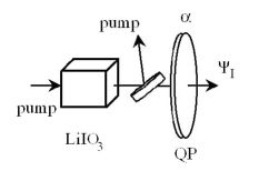
Figure 3: Preparation of states $\Psi_{I}$. The nonlinear crystal generates the basis ququart state(s) via type-I SPDC. Then the state is transformed by the wave plate QP whose parameters depend on its orientation angle $\alpha$.

We used the basis state $|V_{1}V_{2}\rangle$, so the states generated in this way have the following structure:

$$|\Psi_{I}(\alpha)\rangle=\left({{\begin{array}[]{*{20}c}{r_{1}r_{2}\hfill}\\ {r_{1}t_{2}^{*}\hfill}\\ {t_{1}^{*}r_{2}\hfill}\\ {t_{1}^{*}t_{2}^{*}\hfill}\\ \end{array}}}\right).$$ (26)

Since coefficients $r_{j}$ and $t_{j}$ depends on the the orientation angle $\alpha_{j}$ there is a simple way to transform the state by rotating the retardant plate. As we will show below, a usage of a single crystal allows one to prepare the whole sub-set of ququarts which can be used for quantum key distribution.

III.1.2 Entangled states

To prepare the ququarts with $c_{1}c_{4}\neq c_{2}c_{3}$ it was sufficient to use two crystals like it was done when frequency non-degenerated Bell-states have been generated freqBellprep (Fig.4).

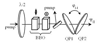
Figure 4: Preparation of states $\Psi_{II}$. Two nonlinear crystals generates pair of the basis ququart states via type-I SPDC. The relative phase between states $\varphi_{14}$ is controled by two quartz plates QP1, QP2. The state amplitudes are controlled with the help of half-lambda plate.

In order to introduce a phase shift $\varphi_{14}$ between horizontally and vertically polarized type-I biphotons two 1 mm quartz plates (QP1,2) that can be rotated along the optical axis were used. By tilting the plates the family of ququarts was generated:

$$|\Psi_{II}(\phi)\rangle=\left({{\begin{array}[]{*{20}c}{|c_{1}|\hfill}\\ {0\hfill}\\ {0\hfill}\\ {|c_{4}|e^{-i\varphi_{14}}\hfill}\\ \end{array}}}\right),$$ (27)

where real amplitudes $|c_{1}|,|c_{4}|$ were controlled by the half wave plate inserted into the linearly polarized pump beam. Some remarkable interference phenomena with $|\Psi_{II}(\phi)\rangle$-like states have been observed. For example, when the phase of $\lambda_{1}$-photon is varied, then modulation with the same wavelength is observed in coincidence rate, while changing the phase of $\lambda_{2}$-photon it is this modulation that is manifested in coincidences freqBellprep . Another effect related to biphotons-ququarts that is widely discussed in quantum optics is ”hidden polarization”. Polarization transformations of frequency non-degenerate Bell-states experimentally have been studied in freqBelltrans .

III.2 Measurement

Basically it is necessary to perform $D^{2}$ independent measurements for complete reconstruction of the arbitrary qudit density matrix. So for $D=4$ the total number of measurements is equal to sixteen. Since the only way to measure biphoton is to register a coincidence of photocounts, we chose a Brown-Twiss scheme supplied with polarization elements to perform projective measurements. A coincidence click that occurs when signals from two detectors fall into the coincidence window is considered a registered event. Since the coincidence click appears at the output with some probability, a statistical treatment of the outcomes becomes very important. Another point that we would like to notice is that according to Bohr’s complementarity principle, there is no way to measure all moments (13, 14) at the same time, dealing with a single ququart only. So to perform a complete set of measurements one needs to generate a lot of representatives of a quantum ensemble.

In order to measure the ququarts we developed two protocols.

III.2.1 Protocol 1.

The idea of the first method is to split the ququart state $|{\Psi_{in}}\rangle$ into two frequency modes and to perform transformations independently on each of the photon from a pair (Fig. 5). Usage of a dichroic beamsplitter allows one to separate frequency modes in space and reduces this protocol to that one developed in Kwiat:01 for two spatially separated polarization qubits. We called this method as ”frequency selective” because frequency mode separation is basically applied to ququart before subjecting it to polarization projective measurements.

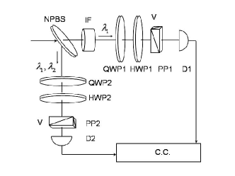
Figure 5: Measurement block for Protocol 1. The Brown-Twiss scheme for measuring intensity correlation between two polarization modes. After spatial separation at the non-polarizing beam splitter (NPBS), signal $(\lambda_{2})$ and idler $(\lambda_{1})$ photons propagate through the quarter- (QWP1,2) and half (HWP1,2) wave plates , polarizing prisms (PP1,2) in two channels. The interference filter (IF) placed in the upper arm and centered at $\lambda_{1}$ selects frequencies modes of ququart. Finally, photons are registered by detectors (D1,2). The coincidence rate from the output of the coincidence circuit (CC) is proportional to the fourth moment in the field $\langle{R}\rangle$.

The polarization transformations can be done using polarization filters placed in front of detectors. Each filter consists of a sequence of quarter- and half-wave plates and a polarization prism, which picks out vertical polarization. In our experiments we kept the protocol developed in Kwiat:01 unchanged, although there are many other configurations of polarization filters leading to the matrix $K_{4}$ reconstruction. Instead of dichroic beamsplitter we used a (50/50)% polarization insensitive beamsplitter and a narrowband filter centered at $\lambda_{1}$ was put in front of the first detector. In such a way we postselected the desirable events in registering coincidences. Approximately in quarter of trials, the photons with central wavelength $\lambda_{1}$ forming a biphoton are going to the first detector, while the conjugated ones (with central wavelength $\lambda_{2}$) are going to the second detector. In the remaining cases, the events are not registered because they either do not contribute to coincidences or corresponding photons do not pass through the interference filter.

In the Heisenberg representation the polarization transformation for each dichroic beam-splitter output port is given by:

$$\left({{\begin{array}[]{*{20}c}{{a_{j}}^{\prime\dagger}\hfill}\\ {{b_{j}}^{\prime\dagger}\hfill}\\ \end{array}}}\right)=\left({{\begin{array}[]{*{20}c}0\hfill&0\hfill\\ 0\hfill&1\hfill\\ \end{array}}}\right)D_{\lambda_{j}/2}({\delta_{j}=\pi/2,\theta})$$ (32)

$$\times D_{\lambda_{j}/4}({\delta_{j}=\pi/4,\chi})\left({{\begin{array}[]{*{20}c}{\frac{1}{\sqrt{2}}\hfill}&0\hfill\\ 0\hfill&{\frac{1}{\sqrt{2}}\hfill}\\ \end{array}}}\right)\left({{\begin{array}[]{*{20}c}{a_{j}^{\dagger}\hfill}\\ {b_{j}^{\dagger}\hfill}\\ \end{array}}}\right).$$ (37)

We designate with $j=1,2$ different output ports of beamsplitter which correspond to different wavelengths $\lambda_{1,2}$. Four $2\times 2$ matrixes in the right-hand side of (37) describe the action of the non-polarizing beam-splitter, $\lambda/4$-, $\lambda/2$- plates and vertical polarization prism on the state vector of each photon;

$$D_{\lambda_{j}/2,\lambda_{j}/4}=\left({{\begin{array}[]{*{20}c}t_{j}\hfill&r_{j}\hfill\\ {-r_{j}^{\ast}\hfill}&{t_{j}^{\ast}\hfill}\\ \end{array}}}\right),$$

where $r_{j}$ and $t_{j}$ - are the coefficients introduced in Eq. (23), so for a $\lambda_{j}/4$-plate ($\delta_{j}=\pi/4$),

$$t_{\lambda_{j}/4}=\frac{1}{\sqrt{2}}({1+i\cos 2\chi_{j}}),r_{\lambda_{j}/4}=\frac{i}{\sqrt{2}}\sin 2\chi_{j}$$ (38a)

and for a $$\lambda_{j}/2 \delta_{j}=\pi/2$$-plate ()

$$t_{\lambda_{j}/2}=i\cos({2\theta_{j}}),r_{\lambda_{j}/2}=i\sin({2\theta_{j}}).$$ (38b)

Thus, there are four real parameters (two for each channel) that determine polarization transformations. Namely, these parameters are orientation angles for two pairs of wave plates: $\theta_{1},\chi_{1},\theta_{2},\chi_{2}.$ Also we would like to notice that there is another parameter that affects strongly on result of polarization transformations. It is a wavelength(s) of down-converted photon(s). For example varying the frequency spectrum of SPDC by tilting a crystal which generates biphotons one can significantly change the transformed state (20) using fixed parameters of the wave plates such as geometrical thickness $h$ and its orientation $\alpha$. This property makes biphoton-based ququarts much more flexible to be controlled than biphoton-qutrits and allows one to choose convenient regimes for operations with them.

As it was mentioned above, the output of the Brown-Twiss scheme is the coincidence rate of the pulses coming from two detectors $D_{1}$ and $D_{2}$. The corresponding moment of the fourth order in the field has the following structure:

$$R_{1,2}\propto\langle{{{b^{\prime}}_{1}}^{\dagger}{{b^{\prime}}_{2}}^{\dagger}{b^{\prime}}_{1}{b^{\prime}}_{2}}\rangle=R({\theta_{1},\chi_{1},\theta_{2},\chi_{2}})$$ (39)

In the most general case this moment contains a linear combination of ten moments (13, 14) forming the matrix $K_{4}$. So the main purpose of the state reconstruction procedure is extracting these moments from the set-up outcomes by varying the four parameters of the polarization Brown-Twiss scheme. Consider some special examples, which give the corresponding lines in the complete protocol introduced below (Table I). The measurement of first four moments (13) is trivial procedure. For instance the third line in the (Table I) corresponds to selection the basis state $|V_{1}V_{2}\rangle$. The other three upper lines correspond to the measurement of other basis states $|H_{1}H_{2}\rangle$, $|H_{1}V_{2}\rangle$, and $|V_{1}H_{2}\rangle$. Remaining lines of protocol show how to measure one of the complex moments (14). To measure the real part of the moment $E$, let us set the wave-plates in the Brown-Twiss scheme in the following way.

The first channel:

$$\lambda/4:\chi_{1}=0^{\circ},D_{\lambda/4}=\frac{1}{\sqrt{2}}\left({{\begin{array}[]{*{20}c}1+i\hfill&0\hfill\\ 0\hfill&1-i\hfill\\ \end{array}}}\right);$$ (40a)

$$\lambda/2:\theta_{1}=45^{\circ},D_{\lambda/2}=\left({{\begin{array}[]{*{20}c}0\hfill&i\hfill\\ i\hfill&0\hfill\\ \end{array}}}\right).$$ (40b)

The second channel:

$$\lambda/4:\chi_{2}=-45^{\circ},D_{\lambda/4}=\frac{1}{\sqrt{2}}\left({{\begin{array}[]{*{20}c}{1\hfill}&-i\hfill\\ -i\hfill&{1\hfill}\\ \end{array}}}\right);$$ (41a)

$$\lambda/2:\theta_{2}=-22.5^{\circ},D_{\lambda/2}=\frac{1}{\sqrt{2}}\left({{\begin{array}[]{*{20}c}i\hfill&-i\hfill\\ -i\hfill&-i\hfill\\ \end{array}}}\right).$$ (41b)

Substituting these matrices into Eq. (28) and taking into account the commutation rules for the creation and annihilation operators it is easy to get the final moment to be measured:

$$R=\langle\Psi|b_{1}^{\dagger}b_{2}^{\dagger}b_{1}b_{2}|\Psi\rangle=1/8({A+C+2\textrm{Re}E}).$$

A complete set of the measurements called the tomography protocol is presented in Table I. Each row corresponds to the setting of the plates to measure the moment highlighted in the sixth column. The last column corresponds to amplitude of the process (see below).

Table 1: Protocol 1. Each line contains orientation of the half ($\theta_{s,i}$) and quarter ($\chi_{s,i}$) wave plates in the measurement block. Last two columns show the corresponding moment $R_{\nu}$ and the process amplitude $M_{\nu}(\nu=1,..16)$. Sign ”-” in orientation of plates for reflection channel is introduced to compensate $\pi$-phase shift occurring by reflectance from the beamsplitter.

	Set-up parameters				Moments to be measured	Amplitude of the process
$\nu$	$\chi_{s}$	$\theta_{s}$	$\chi_{i}$	$\theta_{i}$	$R_{\nu}=|M_{\nu}|^{2}$	$M_{\nu}$
1.	0	$45^{\circ}$	0	$-45^{\circ}$	$A/4$	$c_{1}/2$
2.	0	$45^{\circ}$	0	0	$B/4$	$c_{2}/2$
3.	0	0	0	0	$D/4$	$c_{4}/2$
4.	0	0	0	$-45^{\circ}$	$C/4$	$c_{3}/2$
5.	0	$22.5^{\circ}$	0	$-45^{\circ}$	$1/8(A+C+2\textrm{Im}F)$	$\frac{1}{2\sqrt{2}}(c_{1}-ic_{3})$
6.	0	$22.5^{\circ}$	0	0	$1/8(B+D+2\textrm{Im}K)$	$\frac{1}{2\sqrt{2}}(c_{2}-ic_{4})$
7.	$45^{\circ}$	$22.5^{\circ}$	0	0	$1/8(B+D-2\textrm{Re}K)$	$\frac{1}{2\sqrt{2}}(c_{2}-c_{4})$
8.	$45^{\circ}$	$22.5^{\circ}$	0	$-45^{\circ}$	$1/8(A+C-2\textrm{Re}F)$	$\frac{1}{2\sqrt{2}}(c_{1}-c_{3})$
9.	$45^{\circ}$	$22.5^{\circ}$	0	$-22.5^{\circ}$	$1/16(A+B+C+D)-1/8(\textrm{Im}E+\textrm{Re}F-\textrm{Im}G+\textrm{Im}I+\textrm{Re}K+\textrm{Im}L)$	$\frac{1}{4}[(c_{1}-c_{3})+i(c_{2}-c_{4})]$
10.	$45^{\circ}$	$22.5^{\circ}$	$-45^{\circ}$	$-22.5^{\circ}$	$1/16(A+B+C+D)-1/8(\textrm{Re}F-\textrm{Re}E+\textrm{Re}G+\textrm{Re}I+\textrm{Re}K-\textrm{Re}L)$	$\frac{1}{4}[c_{1}+c_{2}-c_{3}-c_{4}]$
11.	0	$22.5^{\circ}$	$-45^{\circ}$	$-22.5^{\circ}$	$1/16(A+B+C+D)+1/8(\textrm{Im}F+\textrm{Re}E+\textrm{Im}G+\textrm{Im}I+\textrm{Re}L+\textrm{Im}K)$	$\frac{1}{4}[(c_{1}+c_{2})-i(c_{3}+c_{4})]$
12.	0	$45^{\circ}$	$-45^{\circ}$	$-22.5^{\circ}$	$1/8(A+B+2\textrm{Re}E)$	$\frac{1}{2\sqrt{2}}(c_{1}+c_{2})$
13.	0	0	$-45^{\circ}$	$-22.5^{\circ}$	$1/8(C+D+2\textrm{Re}L)$	$\frac{1}{2\sqrt{2}}(c_{3}+c_{4})$
14.	0	0	$-90^{\circ}$	$-22.5^{\circ}$	$1/8(C+D+2\textrm{Im}L)$	$\frac{1}{2\sqrt{2}}(c_{3}-ic_{4})$
15.	0	$45^{\circ}$	$-90^{\circ}$	$-22.5^{\circ}$	$1/8(A+B+2\textrm{Im}E)$	$\frac{1}{2\sqrt{2}}(c_{1}-ic_{2})$
16.	0	$22.5^{\circ}$	$-90^{\circ}$	$-22.5^{\circ}$	$1/16(A+B+C+D)+1/8(\textrm{Im}F+\textrm{Im}E-\textrm{Re}G+\textrm{Re}I+\textrm{Im}L+\textrm{Im}K)$	$\frac{1}{4}[(c_{1}-c_{4})-i(c_{2}+c_{3})]$

Amplitude of the quantum process, corresponding to passing down-converted photons through the measurement set-up for each configuration of wave plates is described by the following equation:

$$M_{\nu}(\delta_{1},\theta_{k},\delta_{2},\varphi_{l})=\frac{1}{2}[a_{1}a_{2}c_{1}+a_{1}b_{2}c_{2}+b_{1}a_{2}c_{3}+b_{1}b_{2}c_{4}].$$ (42)

where

$$\begin{array}[]{cc}a_{1}=-{r_{\lambda/2}}(\theta_{1})t^{*}_{\lambda/4}(\chi_{1})-{t_{\lambda/2}}(\theta_{1})r_{\lambda/4}(\chi_{1}),&\\ a_{2}=-{r_{\lambda/2}}(\theta_{2})t^{*}_{\lambda/4}(\chi_{2})-{t_{\lambda/2}}(\theta_{2})r_{\lambda/4}(\chi_{2}),&\\ b_{1}=-{r_{\lambda/2}}(\theta_{1})r^{*}_{\lambda/4}(\chi_{1})+{t_{\lambda/2}}(\theta_{1})t_{\lambda/4}(\chi_{1}),&\\ b_{2}=-{r_{\lambda/2}}(\theta_{2})r^{*}_{\lambda/4}(\chi_{2})+{t_{\lambda/2}}(\theta_{2})t_{\lambda/4}(\chi_{2}).\end{array}$$ (43)

The complete reconstruction of the input state $|\Psi^{in}\rangle$ was performed according to the algorithm considered in our previous work ourPRA:04 .

Concluding this section we would like to stress that if usual frequency insensitive (broadband) beamsplitter is used and no interference filters are inserted either in front of or behind this beamsplitter, then ”non-selective” method of ququart measurement is possible. In this case one does not need to use the interference filter to select the wavelength in each channel of Brown-Twiss scheme. In other words each detector is allowed to register photons with different frequencies and the fourth moment in the field to be measured becomes

$$R_{1,2}\propto\langle{({{b^{\prime}}_{1}+{b^{\prime}}_{2}})^{\dagger}_{Detector2}({b^{\prime}}_{1}+{b^{\prime}}_{2}})_{Detector1}\rangle$$ (44)

instead of (39). In non-selective method the expression connecting observable value $R_{1,2}$ with components of coherence matrix (13, 14) is bulky and it is not reasonable to utilize it for the state reconstruction. However in particular case we applied non-selective method to ququart reconstruction procedure and developed the special protocol, which is introduced in the next section.

III.2.2 Protocol 2.

In the second protocol the whole ququart state (2) is subjected to the linear transformations using a set of the retardant plates JETPLett . Then projective measurements were applied to the state $|\Psi^{in}\rangle$ after it being transformed by the plates. Using the retardant plates with fixed optical thickness, one can reconstruct the state, varying the orientation of the plates (Fig. 6).

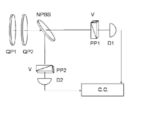
Figure 6: Measurement block for Protocol 2. After the input state is subjected to transformations by wave plates (QP1, QP2), the projective measurements selecting vertical polarizations of ququart components were performed.

Mathematically one needs to derive an equations set connecting real and imaginary parts of moments (13, 14) with coincidence rate. It turns out that the complete set of moments (13, 14) can be extracted from the projective measurements if two different plates were used.

$$|\Psi^{out}\rangle_{kl}=\hat{G}(\delta_{1},\theta_{k})\hat{G}(\delta_{2},\varphi_{l})|\Psi^{in}\rangle,$$ (45)

where $\theta_{k}$ and $\varphi_{l}$ are the orientation angles of the first and second plates. The parameters of the plates, i.e. optical thicknesses for different wavelengths $\delta_{\lambda{j}}^{(1,2)}$ and their orientations are supposed to be known. The projective measurements were realized by means of pair of polarization prisms, transmitting vertical polarization and settled in front of each single photon detector. So the number of coincidences is

$$R_{kl}\propto|\langle V_{1}V_{2}|\Psi_{out}\rangle_{kl}|^{2}.$$ (46)

In order to reconstruct the state it is sufficient to perform at least four measurements corresponding to different orientations of the second plate $\varphi_{l}$ and repeat this procedure at least four times varying orientation of the first plate $\theta_{k}$. But in experiments we performed redundant number of measurements to increase the accuracy and finally used 36 orientation of the second plate. Thus total number of measurements $\mu$ in this protocol was equal to $4\times 36=148$. Therefore the Protocol 2 includes 148 lines instead of 16 lines used in Protocol 1.

III.3 Experimental setup.

For generation of biphoton-based ququarts we used lithium-iodate 15 mm crystal pumped with 5 mW cw- helium-cadmium laser operating at 325 nm. The orientation of the crystal is chosen at $58.98^{\circ}$ with respect to the pump wave vector that the down-converted photons at $\lambda_{1}=702nm$ and $\lambda_{2}=605nm$ had been generated. For some particular cases we selected biphoton-ququarts at wavelengths $\lambda_{1}=667nm$ and $\lambda_{2}=635nm$. Thus the either $|V_{702}V_{605}\rangle$ or $|V_{667}V_{635}\rangle$ states were used as an initial states. Then, this state was subjected to transformations done by dichroic waveplates to prepare the sub-set of ququarts with $c_{1}c_{4}=c_{2}c_{3}$ (26). That sub-set of states was used to be reconstructed. In particular we used the 0.988-mm (or 0.315-mm ) length quartz plate and changed it orientation $\alpha$, which served as a parameter. Since the thickness of the plate, quartz dispersion and orientation $\alpha$ are supposed to be known, we were able to calculate the result of the state transformation with high accuracy. When Protocol 2 was applied for ququart reconstraction we used the quartz plates with thicknesses $0.821mm$ (QP1) and $0.715mm$ (QP2). Both protocols were applied to reconstruct the initial state $|\Psi_{I}(\alpha)\rangle$. In the case when sub-set $c_{1}c_{4}\neq c_{2}c_{3}$ had been generated we used two consecutive 1.8 mm thick type-I BBO (beta-barium borate) crystals whose optical axis are oriented perpendicularly with respect to each other at $36.33^{\circ}$ with respect to the pump wave vector. An interference filter centered either at $702nm$ or at $635nm$ and with a FWHM bandwidth of $3nm$ was placed in transmitted arm to make a spectral selection of one photon of a pair, while the photon with conjugated frequency was sent to a reflected arm. As it was already mentioned above this scheme is equivalent to that one used in Kwiat:01 . The only difference between our scheme and developed in Kwiat:01 resulted from operating with frequency non-degenerate collinear regime of SPDC instead of non-collinear, frequency degenerate regime used in Kwiat:01 . Without loss of generality, this scheme also allows to reconstruct any arbitrary polarization ququart state by registering coincidence rate for different projections that are done by the polarization filters located in each arm. Each filter consists of a zero-order quarter- and half-waveplate and a fixed analyzer. Two Si-APD’s linked to a coincidence scheme with 1.5 nsec time window were used as single photon detectors.

III.4 Results and discussion

We applied both protocols to measure the set of states $\Psi_{I}$, generated with $|V_{667nm}V_{635nm}\rangle$ transformed by quartz plate QP, like it is shown in Fig. 3. We have tested the states which were generated for two orientation angles of plate QP $\alpha=0^{\circ},90^{\circ}$. According to the Protocol 2 four sets of measurements was performed for each input state, so totally we performed 148 measurements of coincidence rate as a function of orientation angles $\varphi_{l}$ of QP1 and $\theta_{k}$ of QP2. The dependence of coincidence rate on the orientation $\varphi_{l}$ for $\theta_{k}=90^{\circ}(a)$, $105^{\circ}(b)$, $120^{\circ}(c)$, and $135^{\circ}(d)$ is shown in Fig. 7 for the input state corresponding to orientation $\alpha=20^{\circ}$ of the plate forming the state.

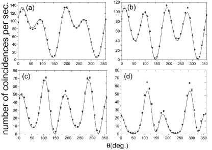
Figure 7: Dependence of coincidence rate on tilting angle ${\theta}$

The solid curve gives the theoretical behavior of the normalized fourth moment, the dots with bars show the experimental data. The tables II-IV show the results of statistical reconstruction of ququarts $|\Psi_{I}\rangle$ performed with root estimation method. The tables show theoretical and experimental four-dimensional state-vectors $c_{theory}$, $c_{exp}$ as well as fidelity $F$ defined by

$$F=|\langle c_{theory}|c_{exp}\rangle|^{2}.$$ (47)

In table II we collected the data measured by Protocol 1 (ququarts with $\lambda_{1}=702nm$ and $\lambda_{2}=605nm$, $h$(QP)=0.315mm). Table III corresponds to measurements performed by Protocol 2 (ququarts with $\lambda_{1}=667nm$ and $\lambda_{2}=635nm$, $h$(QP)=0.988mm). And finally we demonstrate the validity of preparation, transformation, and measurement procedures performed over biphotons-ququarts by reconstruction of the Bell states $|\Phi^{\pm}\rangle$ ($\lambda_{1}=702nm$ and $\lambda_{2}=605nm$), measured along with Protocol 1 and shown in Table IV. As it is seen from the tables the accuracy of state reconstruction is a little bit lower when Protocol 1 has been applied. It results from the fact that Protocol 1 exploits minimal number of measurements (16) which is needed for four-state system reconstruction. At the same time since redundant number of measurements (148) was involved when applying the second protocol, the highest accuracy was achieved like in the case of biphotons-qutrits ourPRA:04 . The respectively low fidelity for Bell states reconstruction (Table IV) is explained by experimental imperfections at the preparation stage. Preliminary estimation of the prepared state quality can be extracted from visibility displayed during interference experiments with these states. For example, typical visibility meaning revealed when space-time interference observed was $0.9$ interference . Another factor limiting the accuracy of the state reconstruction is the finite number of events to be registered. In the case of $|\Psi_{I}\rangle$-set of states we collected about several thousands of coincidences during accumulation time whereas in the case of $|\Psi_{II}\rangle$-set only a few hundreds coincidences were registered in total.

Table 2:

protocol 1
$\alpha$ (deg.)	theory	experiment	$F$
0	0 0 0 1	-0.0295 - 0.0306i 0.0543 - 0.0202i -0.0154 - 0.0093i 0.9972	0.995
10	-0.0015 - 0.0229i 0.0038 - 0.0050i 0.2013 + 0.1735i 0.9638	0.0584 - 0.1926i 0.0073 + 0.0170i 0.1633 + 0.1233i 0.9577	0.963
20	-0.0021 - 0.0386i 0.0154 - 0.0162i 0.3430 + 0.3625i 0.8654	0.0015 - 0.0326i 0.0019 - 0.0660i 0.3967 + 0.2085i 0.8909	0.976
30	-0.0015 - 0.0445i 0.0337 - 0.0225i 0.3530 + 0.5716i 0.7383	-0.0310 - 0.0542i 0.0166 - 0.0416i 0.4526 + 0.5386i 0.7065	0.991
40	-0.0005 - 0.0440i 0.0511 - 0.0116i 0.1601 + 0.7466i 0.6421	0.0112 - 0.0823i 0.1174 - 0.0328i 0.1087 + 0.8363i 0.5167	0.970

Table 3:

protocol 2
$\alpha$ (deg.)	theory	experiment	$F$
0	0 0 0 1	-0.0555-0.0204i -0.0059+0.005i -0.0425+0.0052i 0.9973	0.996
20	0.8097 -0.4568-0.3527i -0.0103-0.0859i -0.0316+0.0529i	0.8067 -0.4847-0.3304i 0.023-0.0554i -0.0174+0.0413i	0.998

Table 4:

protocol 1
theory	experiment	$F$
$0.707$ 0 0 $0.707$	0.7326 0.0818-0.0963i 0.0003-0.0281i 0.6131+0.2657i	0.941
$0.707$ 0 0 -$0.707$	0.6597 0.2518+0.4692i 0.0897-0.0319i -0.6155+0.3261i	0.934

IV Polarization ququarts in QKD protocol

The complete QKD protocol with four-dimensional polarization states exploits five mutually unbiased bases with four states in each mutual . In terms of biphoton states the first three bases consist of product polarization states of two photons and last two bases consist of two-photon entangled states:

$$\begin{array}[]{cc}I.\quad|H_{1}H_{2}\rangle;\quad|H_{1}V_{2}\rangle;\quad|V_{1}H_{2}\rangle;\quad|V_{1}V_{2}\rangle,\\ II.\quad|D_{1}D_{2}\rangle;\quad|D_{1}\overline{D_{2}}\rangle;\quad|\overline{D_{1}}D_{2}\rangle;\quad|\overline{D_{1}}\overline{D_{2}}\rangle,\\ III.\quad|R_{1}R_{2}\rangle;\quad|R_{1}L_{2}\rangle;\quad|L_{1}R_{2}\rangle;\quad|L_{1}L_{2}\rangle,\\ IV.\quad|R_{1}H_{2}\rangle+|L_{1}V_{2}\rangle;\quad|R_{1}H_{2}\rangle-|L_{1}V_{2}\rangle;\\ |L_{1}H_{2}\rangle+|R_{1}V_{2}\rangle;\quad|L_{1}H_{2}\rangle-|R_{1}V_{2}\rangle,\\ V.\quad|H_{1}R_{2}\rangle+|V_{1}L_{2}\rangle;\quad|H_{1}R_{2}\rangle-|V_{1}L_{2}\rangle;\\ |H_{1}L_{2}\rangle+|V_{1}R_{2}\rangle;\quad|H_{1}L_{2}\rangle-|V_{1}R_{2}\rangle.\end{array}$$ (48)

Here $|H\rangle\equiv|1\rangle$, $|V\rangle\equiv|0\rangle$, $|D\rangle\equiv\frac{1}{\sqrt{2}}(|1\rangle+|0\rangle)$, $\overline{D}\equiv\frac{1}{\sqrt{2}}(|1\rangle-|0\rangle)$, $|R\rangle\equiv\frac{1}{\sqrt{2}}(|1\rangle+i|0\rangle)$, $|L\rangle\equiv\frac{1}{\sqrt{2}}(|1\rangle-i|0\rangle)$ indicate horizontal, vertical, +45 linear, -45 linear, right- and left-circular polarization modes correspondingly, and lower indices numerate the frequency modes of two photons. It has been proved Tittel that it is sufficient enough to use only first two or three bases for the efficient QKD. Using incomplete set of bases one sacrifices the security but enhances the key generation rate. Since the realization of Bell measurements for the last two bases requires a big experimental effort on both preparation and measurement stages of a protocol, we will restrict ourselves to first three bases. As we will show experimentally, all states from the first three bases can be prepared with the help of a single non-linear crystal and local unitary transformations. This is fundamental distinction with respect to biphotons-qutrits where SU(2) transformations between states from mutually unbiased bases are prohibited. We also present a measurement scheme that allows to discriminate the states belonging to one basis deterministically thus allowing its implementation in realization of QKD protocol with polarization ququarts.

IV.1 Experimental procedure.

Experimental setup for generation of ququart states belonging first three bases (48) is shown in Fig. 8. To varify the state generated in the set-up either protocol 1 or protocol 2 might be used. Usually we applied protocol 1 for checking the ququart state.

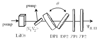
Figure 8: Setup for preparation and measurement of ququarts which can be used in QKD. Wave plates DP1, DP2 oriented at $45^{\circ}$ degrees with respect to vertical axis serve as dichroic retardation plate with variable optical thickness which is controlled by tilting angle $\theta$. Two zero-order plates ZP1, ZP2 allow to chose the basis.

Let us consider as an example, the preparation of a state $|H_{1}V_{2}\rangle$ from the initial state $|V_{1}V_{2}\rangle$. This transformation can be achieved by a dichroic waveplate that introduces a phase shift of $2\pi$ for a vertically polarized photon at $605nm$, a phase shift of $\pi$ for the conjugate photon and that is oriented at $45^{\circ}$ to the vertical direction. Using quarts plates as retardation material it is easy to calculate that the thickness of the waveplate that does this transformation should be equal to $3.406mm$ order . Since these waveplates were not readily available and the result of transformation is extremely sensitive to the small variations of thickness, we used the following method to achieve the desired thickness. Two quartz plates with geometric thicknesses of $3.716mm$ (DP1) and $0.315mm$ (DP2) with orthogonally oriented optical axis were placed consecutively in the biphoton beam. The consecutive action of these two waveplates correspond to the action of quartz waveplate with an effective thickness of $3.401mm$. If then one can tilt these waveplates towards each other by a finite angle $\theta$, then the optical thickness of the effective waveplate, formed by DP1 and DP2 will be changing, and, at a certain value of $\theta$, the desired transformation will be achieved. This corresponds to maximal coincidence rate when the measurement part (protocol 1) is tuned to select a state $|H_{1}V_{2}\rangle$. Monitoring the coincidences, one can obtain the value of ${\theta}$ for which the maximum occurs. Then, fixing the tilting angle at this value, one can perform a complete quantum state tomography protocol in order to verify if the state really coincides with the ideal. In order to change the basis from $I$ to $II(III)$, zero order half- (quarter) waveplates $ZP1$ ($ZP2$) oriented at $22.5^{\circ}(45^{\circ})$ were used. This procedure is repeated for generation of any of the states. Fig. 9.

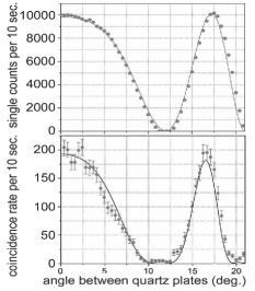
Figure 9: Dependence of single counts (upper) and coincidences (lower) on tilting angle ${\theta}$

shows the coincidences and single count rates versus the change of tilting angle $\theta$ which determines optical thickness of the effective waveplate. If the measurement setup is tuned to select the state $|H_{1}V_{2}\rangle$ then dependence of coincidence rate on the plate optical thicknesses $\delta_{i}$ is given by formula:

$$R_{coin}\propto\langle{{a_{1}}^{\dagger}{b_{2}}^{\dagger}{a}_{1}{b}_{2}}\rangle=\sin^{2}(\delta_{1})\cos^{2}(\delta_{2}),$$ (49)

whereas the single counts distribution in the upper channel is given by

$$I_{702nm}\propto\langle{{a_{1}}^{\dagger}{a}_{1}}\rangle=\sin^{2}(\delta_{1}),$$ (50)

where optical thickness depends on tilting angle as follows:

$$\delta_{j}=\frac{\pi h}{\lambda_{j}}[\frac{(n_{e_{j}})^{2}}{\sqrt{(n_{e_{j}})^{2}-sin^{2}\theta}}-\frac{(n_{o_{j}})^{2}}{\sqrt{(n_{o_{j}})^{2}-sin^{2}\theta}}].$$ (51)

The solid lines in Fig. 9 show the theoretical curves. We performed tomography measurements for the both maxima as well as for the minimum. The minimum in coincidences occurs when intensity in any channel drops to zero, so it is not a necessary condition for distinguishing the orthogonal state to that one selected by given settings of polarization filters. Nevertheless according to calculations and our measurements the minimum in the coincidences at Fig. 9 exactly refers to the state $|V_{1}H_{2}\rangle$. Starting from the $|V_{702nm}V_{605nm}\rangle$, we also prepared and measured the whole set of states from (48) belonging to first three bases. The result of state reconstruction is presented in Table V.

Table 5:

$I$	$|H_{1}H_{2}\rangle$	$|H_{1}V_{2}\rangle$	$|V_{1}H_{2}\rangle$	$|V_{1}V_{2}\rangle$
$F$	0.98	0.94	0.98	0.98
$II$	$|D_{1}D_{2}\rangle$	$|D_{1}\overline{D_{2}}\rangle$	$|\overline{D_{1}}D_{2}\rangle$	$|\overline{D_{1}}\overline{D_{2}}\rangle$
$F$	0.97	0.96	0.95	0.99
$III$	$|R_{1}R_{2}\rangle$	$|R_{1}L_{2}\rangle$	$|L_{1}R_{2}\rangle$	$|L_{1}L_{2}\rangle$
$F$	0.95	0.95	0.96	0.97

At the same time the method discussed in this section allows one to unambiguously distinguish all states forming chosen bases. The measurement set-up which has been already tested in our experiments is shown in the Fig. 10.

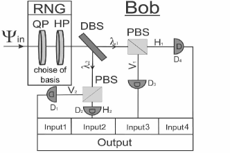
Figure 10: Measurement part at Bob’s station

It consists of the dichroic mirror, separating the photons with different wavelenghts, and a pair of polarization beamsplitters, separating photons with orthogonal polarizations. Four-input double-coincidence scheme linked to the outputs of single-photon detectors registers the biphotons-ququarts. For example for the first basis, the scheme works as follows, provided that Bob’s guess of basis is correct:

if state $|H_{1}H_{2}\rangle$ comes, then detectors D4, D2 will fire,

if state $|H_{1}V_{2}\rangle$ comes, then detectors D4, D1 will fire,

if state $|V_{1}H_{2}\rangle$ comes, then detectors D3, D2 will fire,

if state $|V_{1}V_{2}\rangle$ comes, then detectorsD3, D1 will fire. Same holds for any of the remaining correctly guessed bases, since the quarter- and half waveplates transform the polarization to HV basis in which the measurement is performed. Registered coincidence count from a certain pair of detectors contributes to corresponding diagonal component of the measured density matrix. So if the basis is guessed correctly, then the registered coincidence count deterministically identifies the input state. We illustrate this statement by the table which shows total number of registered events per 30 sec for the input state $|R_{1}L_{2}\rangle$ measured in circular basis and calculated components of experimental (theoretical) density matrix.

Table 6: Coincidence rate and density matrix components

$D_{4}D_{2}$	$\rho_{11}$	$D_{4}D_{1}$	$\rho_{22}$	$D_{3}D_{2}$	$\rho_{33}$	$D_{3}D_{1}$	$\rho_{44}$
$0$	$0.0(0)$	$220$	$0.973(1)$	$6$	$0.027(0)$	$0$	$0.0(0)$

The main obstacle for practical implementation of free-space QKD protocol based on ququarts is that one needs to perform fast polarization transformation at the selected wavelengths. There are different ways how to overcome this problem and we will discuss its elsewhere. In this section we briefly mention the possible ways. Since it is not practical to tune the tilting waveplates every time one wants to encode a quart value, we suggest either to use a polarization modulator that operates on two wavelengths or to split the photons with a dichroic mirrors and perform these transformations on halves of a biphoton independently in a Mach-Zehnder like configuration. It is important to note that interferometric accuracy in Mach-Zehnder is not needed, since it is used only for spatial separation of photons. The practical solution would be to couple the down converted photons in a single mode fiber to ensure a perfect spatial mode overlap and then to split them with wavelength division multiplexer (WDM). Then, the switching between the states can be done with the polarization modulators that introduce a $\pi$ or $2\pi$ phase shifts for the selected wavelength. The choice of basis on Alice’s side is done by a zero order quarter and half waveplates, that can realized within a Pockel (Liquid Crystal) cell driven by randomly selected voltage. Free space communication is proposed since it is not practical to distribute a polarization state within an optical fiber. On Bob’s side, the random choice of basis (RNG) is performed in a same way as on Alice’s side. Then photons are spatially separated with the help of WDM or dichroic mirror and each of the photon is sent to a Brown-Twiss scheme with a polarizing beamsplitter that does a projection of an arrived photon on $H$ or $V$ state as it shown in Fig. 10. Moreover, registering coincidences allows one to circumvent the problem of the detection noise that is common for single-photon based protocols. If the coincidence window is quite small, it is possible to assure a very low level of accidental coincidences for the usual dark count rate of single photon detectors.

To conclude we have suggested and tested a novel method of preparation, and measurement of subset of four-dimensional polarization quantum states. Since for this class of states the polarization degree is not invariant under SU(2) transformations it is possible to switch between orthogonal states using linear transformations like geometrical rotations and phase shifts. We discussed the family of states that can generate the whole basis states using only simple polarization elements and thus might be used in useful applications.

While completing this manuscript we learned about closely related work performed by R. B. R.Adamson and co-authors Steinberg .

Acknowledgments. Stimulating discussions with G.Björk and V.P.Karassiov are gratefully acknowledged. This work was supported in part by Russian Foundation of Basic Research (projects 05-02-16391a, 06-02-16769, 06-02-16393a) and Leading Russian Scientific Schools (project 4586.2006.2).

References

- (1) D.Kaszlikowski, P.Gnasinski, M.Zukowski, W.Miklaszewski, and A.Zeilinger, Phys. Rev. Lett. 85, 4418 (2000); D.Kaszlikowski, D.K.L.Oi, M.Christandl, K.Chang, A.Ekert, L.C.Kwek, and C.H.Oh, Phys. Rev. A. 67 012310 (2003); T.Durt, N.J.Cerf, N.Gisin, and M.Zukowski, Phys. Rev. A. 67, 012311 (2003); D.Collins, N.Gisin, N.Linden, S.Massar, and S.Popescu, Phys. Rev. Lett.88, 040404 (2002).
- (2) H.Bechmann-Pasquinucci, A.Peres, Phys. Rev. Lett. 85, 3313 (2000); D.Bruß, C.Machiavello, Phys. Rev. Lett. 88, 127901 (2002); D.Bruß, C.Macchiavello, Phys. Rev. Lett. 88, 127901 (2002); D.Horoshko, S.Kilin, Optics and Spectroscopy, 94, 691 (2003).
- (3) H.Bechmann-Pasquinucci, W.Tittel, Phys. Rev. A 61, 062308 (2000); M.Bourennane, A.Karlsson, G.Björk, Phys. Rev. A 64, 012306 (2001); N.Cerf, M.Bourennane, A.Karlsson, N.Gisin, Phys. Rev. Lett. 88, 127902 (2002); F.Caruso, H. Bechmann-Pasquinucci, C.Macchiavello, Phys. Rev. A 72, 032340 (2005);
- (4) S.Walborn, D.Lemelle, M.Almeida, and P.Ribeiro, qunt-ph/0510088.
- (5) S.Gröblacher, T.Jennewein, A.Vaziri, G.Weihs, and A.Zeilinger, quant-ph/0511163.
- (6) M.O’Sullivan-Hale, I.Ali Khan, R.Boyd, and J.Howell, Phys. Rev. Lett. 91, 220501 (2005); L.Neves, G.Lima, J.G.Aguirre Gomez, C.H.Monken, C.Saavedra, S.Padua, Phys.Rev.Lett. 94, 100501 (2005).
- (7) A.Vaziri, G.Weihs, and A.Zeilinger, Phys. Rev. Lett. 89, 240401 (2002); A.Vaziri, J.-W.Pan, T.Jennewein, G.Weihs, and A.Zeilinger, Phys.Rev.Lett. 91, 227902 (2003); N.Langford, R.B.Dalton, M.D.Harvey, J.L.O’Brien, G.J.Pryde, A.Gilchrist, S.D.Bartlett, and A.G.White, Phys.Rev.Lett. 93, 053601 (2004).
- (8) H. de Riedmatten, I.Marcikic, V.Scarani, W.Tittel, H.Zbinden, and N.Gisin, Phys. Rev. A 69, 050304 (2004).
- (9) R.T.Thew, A.Acín, H.Zbinden, N.Gisin, Quantum Information and Computation, Vol.4, No.2, 93 (2004), R.T.Thew, A.Acín, H.Zbinden, N.Gisin, Phys. Rev. Lett. 93, 010503 (2004).
- (10) J.C.Howell, A.Lamas-Linares, and D.Bouwmeester, Phys. Rev. Lett. 88, 030401 (2002).
- (11) Yu.Bogdanov, M.Chekhova, S.P.Kulik, G.Maslennikov, M.K.Tey., C.Ch.Oh, Phys. Rev. Lett. 93, 23503 (2004).
- (12) Yu.Bogdanov, M.Chekhova, L.Krivitsky, S.P.Kulik, L.C.Kwek, M.K.Tey, C.Ch.Oh, A.A.Zhukov, Phys. Rev. A 70, 042303 (2004).
- (13) D.N.Klyshko, Photons and Nonlinear Optics, Gordon and Breach, New York (1988).
- (14) A.V.Belinsky and D.N.Klyshko, Laser Phys. 4, 663 (1994).
- (15) D.F.V.James, P.G.Kwiat, W.J.Munro, and A.G.White. Phys. Rev. A 64, 052312 (2001).
- (16) A.V.Burlakov and M.V.Chekhova, JETP Lett. 75, 432 (2002).
- (17) M.V.Chekhova, L.A.Krivitsky, S.P.Kulik, and G.A.Maslennikov, Phys.Rev.A 70, 053801 (2004).
- (18) V.P.Karassiov, J. Phys. A 26, 4345 (1993).
- (19) G.Björk, J.Söderholm, A.Trifonov, P.Usachev, L.L.Sanchez-Soto, and A.V.Klimov, Proc. of SPIE, 4750, 1 (2002); A.Sehat, J.Soderholm, G.Björk, P.Espinoza, A.B.Klimov, L-L.Sanchez-Soto, Phys. Rev. A 71, 033818 (2005).
- (20) D.N.Klyshko, JETP 84, 1065 (1997).
- (21) Of course, it is possible to chose specific orthogonal qutrit states that might be transformed into each other by geometrical rotations and phase shifts. These states are: , , and . According to our definition these states posses whereas its have unit polarization dergee introduced in gunnar . In details the concept of biphoton-qutrits orthogonality and their transformation properties are discussed in ortogonality .
- (22) A.V.Burlakov, S.P.Kulik, Yu.Rytikov, and M.V.Chekhova, JETP, 95 639 (2002).
- (23) L.Mandel and E.Wolf Optical Coherence and Quantum Optics, Cambridge University Press, (1995).
- (24) Y.H.Kim, S.P.Kulik, and Y.Shih. Phys. Rev. A 63, 060301 (2001).
- (25) Yu.I.Bogdanov, R.F.Galeev, S.P.Kulik, G.A.Maslennikov, and E.V.Moreva. JETP Lett. 82, No.3, (2005).
- (26) When studying ”space-time” interference for polarization-type entangled states (27) the dependence of coinceidence rate on phase delay is analized by setting the polarization filters at .
- (27) Bases are mutually unbiased if the inner products between all possible pairs of vectors belonging to different bases, have the same magnitude equal to , where D is the dimension of the Hilbert space.
- (28) The thickness of the retardation plate that performs the transformation is determined by the number of order that is chosen for the specified wavelength according to . Here is the value of the birefringence for the specific wavelength. We chose order for and for .
- (29) R.B.A.Adamson, L.K.Shalm, M.W.Mitchell, and A.M.Steinberg, quant-ph/0601134.