Zeno and anti–Zeno effects for quantum Brownian motion

Abstract

In this paper we investigate the occurrence of the Zeno and anti-Zeno effects for quantum Brownian motion. We single out the parameters of both the system and the reservoir governing the crossover between Zeno and anti-Zeno dynamics. We demonstrate that, for high reservoir temperatures, the short time behaviour of environment induced decoherence is the ultimate responsible for the occurrence of either the Zeno or the anti-Zeno effect. Finally we suggest a way to manipulate the decay rate of the system and to observe a controlled continuous passage from decay suppression to decay acceleration using engineered reservoirs in the trapped ion context .

The quantum Zeno effect (QZE) predicts that the decay of an unstable system can be slowed down by measuring the system frequently enough Misra . In some systems, however, an enhancement of the decay due to frequent measurements, namely the anti-Zeno or inverse Zeno effect (AZE), may occur Lane .

In this paper we focus on the quantum Brownian motion (QBM) model HuPazZhang ; Maniscalco04b ; Weissbook which is a paradigmatic model of the theory of open quantum systems. This model, dealing with the linear interaction of a particle with a bosonic reservoir in thermal equilibrium, is widely used in several physical contexts. It describes the dynamics of a particle interacting with a quantum field in the dipole approximation Zurek , as well as a quantum electromagnetic field propagating in a linear dielectric media Anglin96 . The model is used in nuclear physics to describe, e.g., the two-body decay of an unstable particle Joichi . In quantum chemistry, the QBM model describes the quantum Kramers turnover, which forms the basis of modern theory of activated processes HanggiRev .

Recently, this model has been investigated to explain the loss of quantum coherence (decoherence) due to the interaction between the system and its surroundings. In particular, the absence of macroscopic quantum superpositions in the classical world has been explained, using the QBM model, in terms of environment induced decoherence (EID) Zurek . With the last term we mean here a process which transforms a highly delocalized state in position and/or momentum, e.g. a superposition of coherent states, into a localized classical state.

To the best of our knowledge, the conditions for the occurrence of the quantum Zeno and anti-Zeno effects have never been considered for the QBM model. The aim of this paper is to investigate the Zeno and anti-Zeno phenomena in a system, namely the damped harmonic oscillator, which possesses a classical limit and where it is therefore possible to monitor the transition from quantum to classical dynamics caused by decoherence induced by the environment. Previous studies focus on few level systems and deal with completely quantum states, such as the spin, which have no classical analogue FacchiRev ; Kurizki05 .

Our main result is the demonstration that the occurrence of either the Zeno or the anti-Zeno effect stems from the short time behaviour of the environment induced decoherence, which therefore drives the Zeno–anti-Zeno crossover. On the other hand, one can use the QZE or the AZE to manipulate the quantum-classical border by prolonging or shortening, respectively, the persistence of quantum features in the initial state of the system. Moreover, we suggest a physical context in which the Zeno–anti-Zeno crossover can be observed with current technology by means of reservoir engineering techniques engineerNIST .

The QBM microscopic Hamiltonian model consists of a quantum harmonic oscillator linearly coupled to a quantum reservoir modelled as a collection of non-interacting harmonic oscillators at thermal equilibrium. In the limit of a continuum of frequencies $\omega$, the reservoir properties are described by the reservoir spectral density $J(\omega)$ measuring the microscopic effective coupling strength between the system oscillator and the oscillators of the reservoir.

One of the advantages of the QBM model is that, for factorized initial conditions, it can be described by means of the following exact master equation HuPazZhang ; EPJRWA ; PRAsolanalitica

$$\frac{d\rho_{S}(t)}{dt} = \frac{1}{i\hbar}[H_{0},\rho_{S}(t)]-\Delta(t)[X,[X,\rho_{S}(t)]]$$ (1)

$$+ \Pi(t)[X,[P,\rho_{S}(t)]]+\frac{i}{2}r(t)[X^{2},\rho_{S}(t)]$$

$$- i\gamma(t)[X,\{P,\rho_{S}(t)\}],$$

where $\rho_{S}(t)$ is the reduced density matrix, and $H_{0}=\hbar\omega_{0}\left(a^{{\dagger}}a+\frac{1}{2}\right)$ is the system Hamiltonian, with $a$, $a^{{\dagger}}$, and $\omega_{0}$ the annihilation operator, the creation operator and the frequency of the system oscillator, respectively. Moreover $X=\sqrt{\omega_{0}/2\hbar}\left(a+a^{{\dagger}}\right)$ and $P=i/\sqrt{2\hbar\omega_{0}}\left(a^{{\dagger}}-a\right)$ are the system position and momentum operators, where we have set the mass of the particle $m=1$.

The master equation given by Eq. (1), being exact, describes also the non-Markovian short time system-reservoir correlations due to the finite correlation time of the reservoir. In contrast to other non-Markovian dynamical systems, this master equation is local in time, i.e. it does not contain memory integrals. All the non-Markovian character of the system is contained in the time dependent coefficients appearing in the master equation (for the analytic expression of the coefficients see, e.g., Ref. Maniscalco04b ). These coefficients depend uniquely on the form of the reservoir spectral density. The coefficient $r(t)$ describes a time dependent frequency shift, $\gamma(t)$ is the damping coefficient, $\Delta(t)$ and $\Pi(t)$ are the normal and the anomalous diffusion coefficients, respectively HuPazZhang . In the secular approximation, i.e. after averaging over the rapidly oscillating terms appearing in the dynamics, the only two relevant coefficients are the diffusion coefficient $\Delta(t)$ and the damping coefficient $\gamma(t)$ Maniscalco04b . A simple view of the effect of the diffusion term can be given by looking at the approximate solution HuPazZhang of the master equation given by Eq. (1), in the position space,

$$\rho_{S}(x,x^{\prime},t)\!\simeq\!\rho_{S}(x,x^{\prime},0)\exp\left[-(x-x^{\prime})^{2}\!\!\!\int_{0}^{t}\!\!\!\!\Delta(t_{1})dt_{1}\right]\!\!.$$ (2)

The previous equation shows that the diffusion term is responsible for the vanishing of the off-diagonal terms of the density matrix in position space, i.e. for EID.

For the sake of concreteness, we focus on the case of an Ohmic spectral density with Lorentz-Drude cutoff (see Weissbook , p.25), $J(\omega)=(\omega/\pi)\omega_{c}^{2}/(\omega_{c}^{2}+\omega^{2})$ where $\omega_{c}$ is the cutoff frequency. This form of the spectral density is one of the most commonly used since it leads to a friction force proportional to velocity, which is typical of dissipative systems in several physical contexts. The main result of the paper, however, holds for general forms of the spectral density.

We assume that the system oscillator is initially prepared in one of the eigenstates of its Hamiltonian, i.e. a Fock state $|n\rangle$. During the time evolution the system is subjected to a series of non-selective measurements, i.e. measurements which do not select the different outcomes petruccionebook . We indicate with $\tau$ the time interval between two successive measurements, and we assume that $\tau$ is so short (and/or the coupling so weak) that second order processes may be neglected. Stated another way we assume that the probability $P_{n}(t)$ of finding the system in its initial state $|n\rangle$, i.e. the survival probability, is such that $P_{n}(t)\simeq 1$ and $P_{n}(t)\gg P_{n\pm 1}(t)$. After $N$ measurements the survival probability reads FacchiPRL01 ; FacchiRev

$$P_{n}^{(N)}(t)=P_{n}(\tau)^{N}\equiv\exp\left[-\gamma_{n}^{Z}(\tau)t\right],$$ (3)

where $t=N\tau$ is the effective duration of the experiment and the effective decay rate $\gamma_{n}^{Z}(\tau)$ is defined by the last equality. In Eq. (3), we have assumed that the probability $P_{n}(\tau)$ factorizes. This assumption is justified by the fact that, in the following we will use second order perturbation theory. As shown, e.g., in Ref. Lax , up to second order in the coupling constant, the density matrices of the system and of the environment factorize at all times.

The behaviour of the effective decay rate, appearing in Eq. (3), defines the occurrence of the Zeno or anti-Zeno effect. We indicate with $\gamma_{n}^{0}$ the Markovian decay rate of the survival probability, as predicted by the Fermi Golden Rule. If a finite time $\tau^{*}$ such that $\gamma_{n}^{Z}(\tau^{*})=\gamma_{n}^{0}$ exists, then for $\tau<\tau^{*}$ we have $\gamma_{n}^{Z}(\tau)/\gamma_{n}^{0}<1$, i.e. the measurements hinder the decay (QZE). On the other hand, for $\tau>\tau^{*}$ we have $\gamma_{n}^{Z}(\tau)/\gamma_{n}^{0}>1$ and the measurements enhance the decay (AZE) FacchiPRL01 .

For an initial Fock state $|n\rangle$ there exist two possible decay channels associated with the upward and downward transitions to the states $|n+1\rangle$ and $|n-1\rangle$, respectively. The probability that the oscillator leaves its initial state after a short time interval $\tau$ can be written as $\bar{P}_{n}(\tau)=P_{n}^{\uparrow}(\tau)+P_{n}^{\downarrow}(\tau)$, where $P_{n}^{\uparrow}(\tau)$ and $P_{n}^{\downarrow}(\tau)$ are the probabilities that an upward or a downward transition, respectively, has occurred in the interval of time $0<t<\tau$. From Eq. (12) of Ref. Maniscalco04b , neglecting second order processes, one gets

$$\frac{d\rho_{nn}(t)}{dt}\!=\!-\left\{\!(n\!+\!1)\!\left[\Delta(t)\!-\!\gamma(t)\right]\!+\!n\left[\Delta(t)\!+\!\gamma(t)\right]\right\}\rho_{nn}(t),$$ (4)

where $\rho_{nn}(t)=\langle n|\rho_{S}(t)|n\rangle$. From Eq. (4), noting that $\rho_{nn}(t)\simeq\rho_{nn}(0)$, it is straightforward to see that the upward and downward transition probabilities in the interval $0<t<\tau$ are $P_{n}^{\uparrow}(\tau)=(n+1)\int_{0}^{\tau}[\Delta(t)-\gamma(t)]dt$ and $P_{n}^{\downarrow}(\tau)=n\int_{0}^{\tau}[\Delta(t)+\gamma(t)]dt$, respectively. We note that the survival probability $P_{n}(\tau)$ defined in Eq. (3) is given by $P_{n}(\tau)=1-\bar{P}_{n}(\tau)$. Assuming that $\tau$ is small enough and keeping only the first two terms in the expansion of the exponential appearing in Eq. (3) one easily gets

$$\gamma_{n}^{Z}(\tau)=\frac{1}{\tau}\left[\left(2n+1\right)\int_{0}^{\tau}\Delta(t)dt-\int_{0}^{\tau}\gamma(t)dt\right].$$ (5)

We notice that the quantity $\gamma_{n}^{Z}(\tau)$ can also be derived starting from the generalized master equation obtained in Ref. Facchi05 , applying the formalism to the case of the harmonic oscillator. By definition $\Delta(t)$ and $\gamma(t)$, up to the second order in the coupling constant, are given by HuPazZhang ; Maniscalco04b

$$\!\Delta(t)\!\!\! = \!\!\!\alpha^{2}\!\!\!\!\int_{0}^{t}\!\!\!\!\int_{0}^{\infty}\!\!\!\!\!\!\!\!J(\!\omega\!)\!\coth\!\!\left(\!\hbar\omega/2k_{B}T\!\right)\!\cos(\omega t_{1}\!)\!\cos(\omega_{0}t_{1}\!)d\omega dt_{1},$$ (6)

$$\gamma(t)\!\! = \alpha^{2}\int_{0}^{t}\!\!\int_{0}^{\infty}\!\!\!J(\omega)\sin(\omega t_{1})\sin(\omega_{0}t_{1})d\omega dt_{1},$$ (7)

with $\alpha$ microscopic dimensionless system-reservoir coupling constant. We note that, for high reservoir temperatures $T$, $\Delta(t)\gg\gamma(t)$. Inserting Eqs. (6)-(7) into Eq. (5) and carrying out the double time integration, one obtains

$$\gamma_{n}^{Z}(\tau)\!\!=\!\!\tau\!\!\int_{0}^{\infty}\!\!\!\!\!\!\!J(\omega)\left\{n^{(-)}_{\omega}{\rm sinc}^{2}\!\!\!\left(\omega_{-}\tau\right)+n^{(+)}_{\omega}{\rm sinc}^{2}\!\!\!\left(\omega_{+}\tau\right)\right\}d\omega,$$ (8)

with ${\rm sinc}(x)=\sin(x)/x$, $\omega_{\pm}=(\omega\pm\omega_{0})/2$, and $n^{(\pm)}_{\omega}=\alpha^{2}[\coth\left(\hbar\omega/2k_{B}T\right)(n+1/2)\pm 1]$. In the limit $\tau\rightarrow\infty$ one gets the Markovian value of the effective decay rate $\gamma_{n}^{0}=(2n+1)\Delta_{M}+\gamma_{M}$, with $\Delta_{M}$ and $\gamma_{M}$ Markovian values of the diffusion and damping coefficients respectively.

The quantity ruling the occurrence of either the QZE or the AZE is the ratio

$$\frac{\gamma_{n}^{Z}(\tau)}{\gamma_{n}^{0}}=\frac{\left(2n+1\right)\int_{0}^{\tau}\Delta(t)dt-\int_{0}^{\tau}\gamma(t)dt}{\tau[(2n+1)\Delta_{M}-\gamma_{M}]}.$$ (9)

It is worth underlining that, in general, this quantity depends on the initial state of the system, i.e. on the initial Fock state $|n\rangle$. For high $T$, however, since $\Delta(t)\gg\gamma(t)$, Eq. (9) becomes independent of the initial state

$$\frac{\gamma_{n}^{Z}(\tau)}{\gamma_{n}^{0}} \simeq \frac{\int_{0}^{\tau}\Delta(t)dt}{\tau\Delta_{M}}.$$ (10)

Equation (10) approximates Eq. (9) also for initial highly excited Fock states, i.e. $n\gg 1$. This equation, together with Eq. (9), establishes a connection between two fundamental phenomena of quantum theory, namely the quantum Zeno effects and environment induced decoherence. This connection and its physical consequences, which will be carefully described in the rest of the paper, constitute our main result. We underline that, in deriving Eqs. (9)-(10), no assumption on the form of the spectral density has been done.

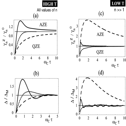
Figure 1: (a) Ratio between the effective decay rate $\gamma_{n}^{Z}(\tau)$ and the Markovian decay rate $\gamma^{n}_{0}$ for high $T$. Solid line $r=0.5$, dotted line $r=1$, dashed line $r=10$. (b) Ratio between the diffusion coefficient $\Delta(\tau)$ and its Markovian value $\Delta_{M}$ for high $T$. Solid line $r=0.5$, dotted line $r=1$, dashed line $r=10$. (c) Ratio between the effective decay rate $\gamma_{n}^{Z}(\tau)$ and the Markovian decay rate $\gamma^{n}_{0}$ for $T\simeq 0$ and $n\gg 1$. Solid line $r=0.1$, dotted line $r=0.5$, dashed line $r=10$. (d) Ratio between the diffusion coefficient $\Delta(\tau)$ and its Markovian value $\Delta_{M}$ for $T\simeq 0$. Solid line $r=0.1$, dotted line $r=0.5$, dashed line $r=10$. A comparison between (a) and (c) shows the temperature dependence of the Zeno–anti-Zeno crossover.

Equation (10) tells us that, for high $T$ reservoirs and/or $n\gg 1$ the effective decay rate depends only on the diffusion coefficient $\Delta(t)$, which in turn describes EID. This yields a new physical explanation of the occurrence of either Zeno or anti-Zeno effects for QBM . The eigenstates of the quantum harmonic oscillator are highly nonclassical states. They are not localized, either in position or in momentum, and therefore they are very sensitive to environment induced decoherence. If the average EID in the interval between two measurements, quantified by $\int_{0}^{\tau}\Delta(t)dt/\tau$, is smaller than the Markovian one, quantified by $\Delta_{M}$, then when the system “restarts”  the evolution after each measurement, the effect of EID is again less than in the Markovian case. Essentially the measurements force the system to experience repeatedly an effective EID which is less strong than the Markovian one. In this case the QZE occurs. On the contrary, whenever the average increase of EID in the interval between two measurements is greater than its Markovian value, then the measurements force the system to experience always a stronger decoherence, and hence the system decay is accelerated (AZE).

An important consequence of Eq. (10) is that the quantum–classical border can be manipulated by means of the QZE and of the AZE. When the QZE occurs, indeed, an initial delocalized state of the harmonic oscillator such as its energy eigenstate remains delocalized for longer times, hence the QZE “moves forward in time”  the quantum–classical border. The opposite situation happens when the AZE occurs.

The analytic expression of the diffusion coefficient allows us to single out the relevant system and reservoir parameters ruling the crossover between the QZE and the AZE. The time $\tau^{*}$ at which $\gamma^{Z}(\tau^{*})=\gamma_{0}$, when it exists and is finite, can be seen as a transition time between Zeno and anti-Zeno phenomena FacchiPRL01 . Our analysis shows that there exist two other relevant parameters, namely the ratio $r=\omega_{c}/\omega_{0}$, quantifying the asymmetry of the spectral distribution, and the ratio $k_{B}T/\hbar\omega_{0}$. For a fixed time interval $\tau$, a change in the values of $r$ and $T$ may lead to a passage from Zeno dynamics to anti-Zeno dynamics and vice versa.

For high $T$, it is easy to prove that a Zeno–anti-Zeno crossover exists only for values of $r<1$, i.e. for $\omega_{0}>\omega_{c}$, as it is shown in Fig 1 (a). This can be understood in terms of EID by looking at the short time dynamics of $\Delta(t)$ in the time interval $0<t<\tau$, i.e. before the first measurement is performed (see Fig. 1 (b)).

The situation changes drastically for the case of a zero-$T$ reservoir, characterized by an asymmetric spectral density. For $n\gg 1$, indeed, in contrast to the high $T$ case, the Zeno–anti-Zeno crossover exists also for values of $r\gg 1$. i.e. in the case $\omega_{0}\ll\omega_{c}$. The region in which only Zeno dynamics may occur now appears at the edge of the spectral density function, i.e. for $\omega_{0}\simeq\omega_{c}$. The reason of such a different dynamics for small values of $\omega_{0}$ stems from the strong decoherence, showing up at low temperatures not only when $r\ll 1$ (as in the high $T$ case), but also for $r\gg 1$ (See Figs. 1 (c)-(d)). Summarizing, the occurrence of the Zeno or anti-Zeno effects is directly related to the absence or presence, respectively, of the so-called initial jolt of the diffusion coefficient $\Delta(t)$ HuPazZhang , which is the signal of strong initial decoherence.

Another interesting aspect stemming from our results concerns the Zeno-anti–Zeno crossover for an initial ground state ($n=0$) of the system oscillator. The high $T$ behaviour is given by Eq. (10) [See Fig. 1 (a)-(b)]. For very low reservoir temperatures ($T\simeq 0$), $\Delta_{M}\simeq\gamma_{M}$ and therefore the denominator of Eq. (9) approaches zero, implying that $\gamma^{Z}(\tau)/\gamma_{0}\gg 1$ always, i.e. the measurements always enhance the decay (AZE). Summarizing, in this case, by changing the reservoir temperature, e.g. starting from high $T$ and lowering the temperature, one observes a passage from the situation depicted in Fig. 1 (a) to a situation in which only the AZE is practically observable.

The possibility of controlling both the environment and the system-environment coupling would allow one to monitor the transition from Zeno to anti-Zeno dynamics. The use of artificial controllable engineered environments has been recently demonstrated for single trapped ions engineerNIST . In Ref. Maniscalco04a it has been shown that the engineered amplitude reservoir realized by applying noisy electric fields to the trap electrodes in engineerNIST can be used to simulate quantum Brownian motion and to reveal the quadratic short time dynamics. Shuttering these noisy electric fields one could model a fast switch off–on of the environment. Actually, when the noise is off, the reservoir simply does not exist anymore. The action of the sudden switch off-on of the environment may be seen as a physical implementation of the operation of trace over the reservoir degrees of freedom. The operation of trace is a typical example of a non-selective measurement (see, e.g., Ref. petruccionebook , p. 321). Hence a succession of short switch off-on periods, realized by shuttering the engineered applied noise, would induce Zeno or anti-Zeno dynamics depending on the value of the system and reservoir parameters and of the shuttering period. This is the core idea for monitoring the Zeno–anti-Zeno crossover with trapped ions.

It is worth underlining that since the measurements causing the acceleration or inhibition of the decay, implemented by a fast switch off-on of the noisy electric field, are non-selective, they do not disturb the vibrational state of the ion. Therefore, by using the set up of Ref. engineerNIST , a comparison between the population $P_{n}^{(N)}(t)$ of the initial vibrational state (e.g. the vibrational ground state $|n=0\rangle$) in presence of shuttered noise (with $N$ the number of switching off-on periods), and the population $P_{n}(t)$ in presence of un-shuttered noise, would show that $P_{n}^{(N)}(t)>P_{n}(t)$ (QZE) or $P_{n}^{(N)}(t)<P_{n}(t)$ (AZE) depending on the choice of the parameters.

All the parameters $\omega_{0}$, $\omega_{c}$, $T$ and $\tau$, driving the Zeno–anti-Zeno crossover, may be varied in the experiments. Although the value of $\omega_{0}$ may be modified only within a certain range and under certain constrains, the modification of both $\omega_{c}$ and $T$ may be obtained by simply filtering the applied noise and varying the noise fluctuations, respectively Maniscalco04a . Since all the parameters ruling the Zeno – anti-Zeno crossover are easily adjustable in the experiments, its observation in the trapped ion context should be already in the grasp of the experimentalists.

The authors acknowledge financial support from the Academy of Finland (projects 207614, 206108, 108699,105740), the Magnus Ehrnrooth Foundation, and the EU’s project CAMEL (Grant No. MTKD-CT-2004-014427). Stimulating discussions with David Wineland, Paolo Facchi and Saverio Pascazio are gratefully acknowledged.

References

- (1) B. Misra and E.C.G. Sudarshan, J. Math. Phys. 18, 756 (1977).
- (2) A.M. Lane, Phys. Lett. A 99, 359 (1983); W.C. Schieve, L.P. Horwits, and J. Levitan, Phys. Lett. A 136, 264 (1989); A.G. Kofman and G. Kurizki, Nature (London) 405, 546 (2000).
- (3) B.L. Hu, J.P. Paz, and Y. Zhang, Phys. Rev. D 45 2843 (1992).
- (4) S. Maniscalco, J. Piilo, F. Intravaia, F. Petruccione, and A. Messina, Phys. Rev. A 70, 032113 (2004).
- (5) U. Weiss, Quantum Dissipative Systems, 2nd edition (World Scientific Publishing, Singapore, 1999).
- (6) W.H. Zurek, Rev. Mod. Phys. 75, 715 (2003).
- (7) J.R. Anglin, and W.H. Zurek, Phys. Rev. D 53, 7327 (1996).
- (8) I. Joichi, Sh. Matsumoto, and M. Yoshimura, Phys. Rev. A 57, 798-804 (1998).
- (9) P. Hänggi, P. Talkner, and M. Borkovec, Rev. Mod. Phys. 62, 251-341 (1990).
- (10) P. Facchi and S. Pascazio, in Progress in Optics, edited by E. Wolf (Elsevier, Amsterdam, 2001), Vol. 42, Chap. 3, p. 147.
- (11) G. Gordon, G. Kurizki, A.G. Kofman, and S. Pellegrin, J. Quant. Inf. Comp. 5, 285 (2005).
- (12) C. J. Myatt et al., Nature 403, 269 (2000); Q.A. Turchette et al., Phys. Rev. A 62, 053807 (2000).
- (13) F. Intravaia, S. Maniscalco, and A. Messina, Eur. Phys. J. B 32, 97 (2003).
- (14) F. Intravaia, S. Maniscalco, and A. Messina, Phys. Rev. A 67, 042108 (2003).
- (15) H.-P. Breuer and F. Petruccione, The Theory of Open Quantum systems (Oxford University Press, 2002).
- (16) P. Facchi, H. Nakazato, and S. Pascazio, Phys. Rev. Lett. 86, 2699 (2001).
- (17) M. Lax, Phys. Rev. 145, 110 (1966).
- (18) P. Facchi et al., Phys. Rev. A 71, 022302 (2005).
- (19) S. Maniscalco , J. Piilo, F. Intravaia, F. Petruccione, and A. Messina, Phys. Rev. A 69, 052101 (2004).