One-and-a-half quantum de Finetti theorems

Abstract

When $n-k$ systems of an $n$-partite permutation-invariant state are traced out, the resulting state can be approximated by a convex combination of tensor product states. This is the quantum de Finetti theorem. In this paper, we show that an upper bound on the trace distance of this approximation is given by $2\frac{kd^{2}}{n}$, where $d$ is the dimension of the individual system, thereby improving previously known bounds. Our result follows from a more general approximation theorem for representations of the unitary group. Consider a pure state that lies in the irreducible representation $U_{\mu+\nu}\subset U_{\mu}\otimes U_{\nu}$ of the unitary group $\mathsf{U}(d)$, for highest weights $\mu$, $\nu$ and $\mu+\nu$. Let $\xi_{\mu}$ be the state obtained by tracing out $U_{\nu}$. Then $\xi_{\mu}$ is close to a convex combination of the coherent states $U_{\mu}(g)|v_{\mu}\rangle$, where $g\in\mathsf{U}(d)$ and $|v_{\mu}\rangle$ is the highest weight vector in $U_{\mu}$.

For the class of symmetric Werner states, which are invariant under both the permutation and unitary groups, we give a second de Finetti-style theorem (our “half” theorem). It arises from a combinatorial formula for the distance of certain special symmetric Werner states to states of fixed spectrum, making a connection to the recently defined shifted Schur functions OkoOls96 . This formula also provides us with useful examples that allow us to conclude that finite quantum de Finetti theorems (unlike their classical counterparts) must depend on the dimension $d$. The last part of this paper analyses the structure of the set of symmetric Werner states and shows that the product states in this set do not form a polytope in general.

I Introduction

There is a famous theorem about classical probability distributions, the de Finetti theorem deFinetti37 , whose quantum analogue has stirred up some interest recently. The original theorem states that a symmetric probability distribution of $k$ random variables, $P^{(k)}_{X_{1}\cdots X_{k}}$, that is infinitely exchangeable, i.e. can be extended to an $n$-partite symmetric distribution for all $n>k$, can be written as a convex combination of identical product distributions, i.e. for all $x_{1},\ldots,x_{k}$

$$P_{X_{1}\cdots X_{k}}(x_{1},\ldots,x_{k})=\int P_{X}(x_{1})\cdots P_{X}(x_{k})d\mu(P_{X}),$$ (1)

where $\mu$ is a measure on the set of probability distributions, $P_{X}$, of one variable. In the quantum analogue stormer ; HudMoo76 ; petz ; cavesfuchsschack ; fuchsschacksecond ; FuScSc04 a state $\rho^{k}$ on $\mathcal{H}^{\otimes k}$ is said to be infinitely exchangeable if it is symmetric (or permutation-invariant), i.e. $\pi\rho^{k}\pi^{\dagger}=\rho^{k}$ for all $\pi\in S_{k}$ and, for all $n>k$, there is a symmetric state $\rho^{n}$ on $\mathcal{H}^{\otimes n}$ with $\rho^{k}=\mathsf{tr}_{n-k}\rho^{n}$. The theorem then states that

$$\rho^{k}=\int\sigma^{\otimes k}dm(\sigma)$$ (2)

for a measure $m$ on the set of states on $\mathcal{H}$.

However, the versions of this theorem that have the greatest promise for applications relax the strong assumption of infinite exchangeability KoeRen05 ; Ren05 . For instance, one can assume that $\rho^{k}$ is $n$-exchangeable for some specific $n>k$, viz. that $\rho^{k}=\mathsf{tr}_{n-k}\rho^{n}$ for some symmetric state $\rho^{n}$. In that case, the exact statement in equation (2) is replaced by an approximation

$$\rho^{k}\approx\int\sigma^{\otimes k}dm(\sigma),$$ (3)

as proved in KoeRen05 , where it was shown that the error is bounded by an expression proportional to $\frac{kd^{6}}{\sqrt{n-k}}$.

Our paper is structured as follows. In section II we derive an approximation theorem for states in spaces of irreducible representations of the unitary group. Our main application of this theorem is an improvement of the error bound in the approximation in  (3) to $2\frac{kd}{n}$ for Bose-symmetric states and to $2\frac{kd^{2}}{n}$ for arbitrary permutation-invariant states. The last step from Bose-symmetry to permutation-invariance is achieved by embedding permutation-invariant states into the symmetric subspace, a technique which might be of independent interest. We conclude this section with a discussion of the optimality of our bounds and explain how our results can be generalised to permutation-symmetry with respect to an additional system.

In section III, we prove the “half” theorem of our title. This refers to a de Finetti theorem for a particular class of states, the symmetric Werner states Werner89 , which are invariant under the action on the tensor product space of both the unitary and symmetric groups. In order to prove our result we derive an exact combinatorial expression for the distance of extremal $n$-exchangeable Werner states to product states of fixed spectrum. This has some mathematical interest because of the connection it makes with shifted Schur functions OkoOls96 . It also provides us with a rich supply of examples that can be used to test the tightness of the bounds of the error in equation (3) and, in section  IV, to explore the structure of the set of convex combinations of tensor product states.

II On Coherent States and the de Finetti theorem

II.1 Approximation by coherent states

In order to state our result we need to introduce some notation from Lie group theory CarterSegalMacDonald95 . Let $\mathsf{U}(d)$ be the unitary group and fix a basis $\{|i\rangle\}_{i=0}^{d-1}$ of $\mathbb{C}^{d}$ in order to distinguish the diagonal matrices with respect to this basis as the Cartan subgroup $\mathsf{H}(d)$ of $\mathsf{U}(d)$. A weight vector with weight $\lambda=(\lambda_{1},\ldots,\lambda_{d})$, where each $\lambda_{i}$ is an integer, is a vector $|v\rangle$ in the representation $U$ of $\mathsf{U}(d)$ satisfying $U(h)|v\rangle=\prod h_{i}^{\lambda_{i}}|v\rangle$, where $h_{1},\ldots,h_{d}$ are the diagonal entries of $h\in\mathsf{H}(d)$. We can equip the set of weights with an ordering: $\lambda$ is said to be (lexicographically) higher than $\lambda^{\prime}$ if $\lambda_{i}>\lambda^{\prime}_{i}$ for the smallest $i$ with $\lambda_{i}\neq\lambda^{\prime}_{i}$. It is a fundamental fact of representation theory that every irreducible representations of $\mathsf{U}(d)$ has a unique highest weight vector (up to scaling); the corresponding weights must be dominant, i.e. $\lambda_{i}\geq\lambda_{i+1}$. Two irreducible representations are equivalent if and only if they have identical highest weights. It is therefore convenient to label irreducible representations by their highest weights and write $U_{\lambda}$ for the irreducible representation of $\mathsf{U}(d)$ with highest weight $\lambda$. It will also be convenient to choose the normalisation of the highest weight vector $|v_{\lambda}\rangle$ to be $\langle v_{\lambda}|v_{\lambda}\rangle=1$ in order to be able to view $|v_{\lambda}\rangle\langle v_{\lambda}|$ as a quantum state.

Given two irreducible representations $U_{\mu}$ and $U_{\nu}$ with corresponding spaces $\mathcal{U}_{\mu}$ and $\mathcal{U}_{\nu}$ we can define the tensor product representation $U_{\mu}\otimes U_{\nu}$ acting on $\mathcal{U}_{\mu}\otimes\mathcal{U}_{\nu}$ by

$$(U_{\mu}\otimes U_{\nu})(g)=U_{\mu}(g)\otimes U_{\nu}(g),$$

for any $g\in\mathsf{U}(d)$. In general this representation is reducible and decomposes as

$$U_{\mu}\otimes U_{\nu}\cong\bigoplus_{\lambda}c_{\mu\nu}^{\lambda}U_{\lambda}.$$

The multiplicities $c_{\mu\nu}^{\lambda}$ are known as Littlewood-Richardson coefficients. It follows from the definition of the tensor product that $|v_{\mu}\rangle\otimes|v_{\nu}\rangle$ is a vector of weight $\mu+\nu$, where $(\mu+\nu)_{i}=\mu_{i}+\nu_{i}$. By the ordering of the weights, $\mu+\nu$ is the highest weight in $U_{\mu}\otimes U_{\nu}$ and $|v_{\mu}\rangle\otimes|v_{\nu}\rangle$ is the only vector with this weight. We therefore identify $|v_{\mu+\nu}\rangle$ with $|v_{\mu}\rangle\otimes|v_{\nu}\rangle$ and remark that $U_{\mu+\nu}$ appears exactly once in $U_{\mu}\otimes U_{\nu}$.

Our first result is an approximation theorem for states in the spaces of irreducible representations of $\mathsf{U}(d)$. Consider a normalised vector $|\Psi\rangle$ in the space $\mathcal{U}_{\mu+\nu}$ of the irreducible representation $U_{\mu+\nu}$. By the above discussion we can embed $U_{\mu+\nu}$ uniquely into the tensor product representation $U_{\mu}\otimes U_{\nu}$. This allows us to define the reduced state of $|\Psi\rangle$ on $\mathcal{U}_{\mu}$ by $\xi_{\mu}=\mathsf{tr}_{\nu}|\Psi\rangle\langle\Psi|$. We shall prove that the reduced state on $\mathcal{U}_{\mu}$ is approximated by convex combinations of rotated highest weight states:

Definition II.1.

For $g\in\mathsf{U}(d)$, let $|v_{\mu}^{g}\rangle:=U_{\mu}(g)|v^{\mu}\rangle$ be the rotated highest weight vector in $\mathcal{U}_{\mu}$. Let $\mathcal{P}_{\mu}(\mathbb{C}^{d})$ be the set of states of the form $\int|v_{\mu}^{g}\rangle\langle v_{\mu}^{g}|dm(g)$, where $m$ is a probability measure on $\mathsf{U}(d)$.

Here, the states $|v_{\mu}^{g}\rangle$, with $g\in\mathsf{U}(d)$, are coherent states in the sense of Perelomov86 . For $d=2$ and $\mu=(k,0)\equiv(k)$, these states are the well-known $\mathsf{SU}(2)$-coherent states.

In the following theorem, we use the trace distance, which is induced by the trace norm $\|A\|:=\frac{1}{2}\mathsf{tr}|A|$ on the set of hermitian operators.

Theorem II.2 (Approximation by coherent states).

Let $|\Psi\rangle$ be in $\mathcal{U}_{\mu+\nu}$ which we consider to be embedded into $\mathcal{U}_{\mu}\otimes\mathcal{U}_{\nu}$ as described above. Then $\xi_{\mu}=\mathsf{tr}_{\nu}|\Psi\rangle\langle\Psi|$ is $\varepsilon$-close to $\mathcal{P}_{\mu}(\mathbb{C}^{d})$, where $\varepsilon:=2(1-\frac{\dim U^{d}_{\nu}}{\dim U^{d}_{\mu+\nu}})$. That is, there exists a probability measure $m$ on $\mathsf{U}(d)$ such that

$$\|\xi_{\mu}-\int|v_{\mu}^{g}\rangle\langle v_{\mu}^{g}|dm(g)\|\leq\varepsilon\ .$$

Proof.

By the definition of $|v^{g}_{\tau}\rangle$ and Schur’s lemma, the operators $E^{g}_{\tau}:=\dim U_{\tau}|v^{g}_{\tau}\rangle\langle v^{g}_{\tau}|$, $g\in\mathsf{U}(d)$ together with the normalised uniform (Haar) measure $dg$ on $U(d)$ form a POVM on $\mathcal{U}_{\tau}$, i.e.,

$$\int E^{g}_{\tau}dg=\openone_{\mathcal{U}_{\tau}}\ .$$ (4)

This allows us to write

$$\xi_{\mu}=\int w_{g}\xi^{g}_{\mu}dg\ ,$$ (5)

where $\xi^{g}_{\mu}$ is the residual state on $\mathcal{U}_{\mu}$ obtained when applying $\{E^{g}_{\nu}\}$ to $|\Psi\rangle$, i.e.,

$$w_{g}\xi_{\mu}^{g}=\mathsf{tr}_{\nu}((\openone_{\mathcal{U}_{\mu}}\otimes E^{g}_{\nu})|\Psi\rangle\langle\Psi|)\ ,$$

where $w_{g}dg$ determines the probability of outcomes.

We claim that $\xi_{\mu}$ is close to a convex combination of the states $|v^{g}_{\mu}\rangle$, with coefficients corresponding to the outcome probabilities when measuring $|\Psi\rangle$ with $\{E^{g}_{\mu+\nu}\}$. That is, we show that the probability measure $m$ on $\mathsf{U}(d)$ in the statement of the theorem can be defined as $dm(g):=\mathsf{tr}(E^{g}_{\mu+\nu}|\Psi\rangle\langle\Psi|)dg$. Our goal is thus to estimate

$$\|\xi_{\mu}-\int\mathsf{tr}(E^{g}_{\mu+\nu}|\Psi\rangle\langle\Psi|)|v^{g}_{\mu}\rangle\langle v^{g}_{\mu}|dg\| =\|S-\delta\|\ ,$$

where, using (5),

$$S :=\int w_{g}\xi^{g}_{\mu}-\frac{\dim U_{\nu}}{\dim U_{\mu+\nu}}\mathsf{tr}(E^{g}_{\mu+\nu}|\Psi\rangle\langle\Psi|)|v^{g}_{\mu}\rangle\langle v^{g}_{\mu}|dg\ ,$$

$$\delta :=(1-\frac{\dim U_{\nu}}{\dim U_{\mu+\nu}})\int\mathsf{tr}(E^{g}_{\mu+\nu}|\Psi\rangle\langle\Psi|)|v^{g}_{\mu}\rangle\langle v^{g}_{\mu}|dg\ .$$

Because $\|\delta\|=\frac{1}{2}(1-\frac{\dim U_{\nu}}{\dim U_{\mu+\nu}})$, it suffices to show that $\|S\|\leq\frac{3}{2}(1-\frac{\dim U_{\nu}}{\dim U_{\mu+\nu}})$. Since $U_{\mu+\nu}\subset U_{\mu}\otimes U_{\nu}$ and $|v_{\mu}\rangle\otimes|v_{\nu}\rangle=|v_{\mu+\nu}\rangle$, we have

$$\frac{\dim U_{\nu}}{\dim U_{\mu+\nu}}\mathsf{tr}(E^{g}_{\mu+\nu}|\Psi\rangle\langle\Psi|) =\langle v^{g}_{\mu}|\mathsf{tr}_{\nu}((\openone_{\mu}\otimes E^{g}_{\nu})|\Psi\rangle\langle\Psi|)|v^{g}_{\mu}\rangle$$

$$=w_{g}\langle v^{g}_{\mu}|\xi^{g}_{\mu}|v^{g}_{\mu}\rangle.$$

So

$$S=\int w_{g}\bigl{(}\xi^{g}_{\mu}-|v^{g}_{\mu}\rangle\langle v^{g}_{\mu}|\xi^{g}_{\mu}|v^{g}_{\mu}\rangle\langle v^{g}_{\mu}|\bigr{)}dg$$ (6)

Now, for all operators $A,B$, we have

$$A-BAB=(A-BA)+(A-AB)-(\openone-B)A(\openone-B)\ ,$$

so putting $A=\xi_{\mu}^{g}$ and $B=|v^{g}_{\mu}\rangle\langle v^{g}_{\mu}|$ in (6), we have

$$S=\alpha+\beta-\gamma,$$

where

$$\alpha :=\int w_{g}(\xi^{g}_{\mu}-|v^{g}_{\mu}\rangle\langle v^{g}_{\mu}|\xi^{g}_{\mu})dg$$

$$\beta :=\int w_{g}(\xi^{g}_{\mu}-\xi^{g}_{\mu}|v^{g}_{\mu}\rangle\langle v^{g}_{\mu}|)dg$$

$$\gamma :=\int w_{g}(\openone_{U_{\mu}}-|v^{g}_{\mu}\rangle\langle v^{g}_{\mu}|)\xi^{g}_{\mu}(\openone_{U_{\mu}}-|v^{g}_{\mu}\rangle\langle v^{g}_{\mu}|)dg.$$

Combining $w_{g}|v^{g}_{\mu}\rangle\langle v^{g}_{\mu}|\xi^{g}_{\mu}=\mathsf{tr}_{\nu}\big{(}(|v^{g}_{\mu}\rangle\langle v^{g}_{\mu}|\otimes E^{g}_{\nu})|\Psi\rangle\langle\Psi|\big{)}=\frac{\dim U_{\nu}}{\dim U_{\mu+\nu}}\mathsf{tr}_{\nu}E^{g}_{\mu+\nu}|\Psi\rangle\langle\Psi|$ with (4) and (5), we get

$$\alpha =\bigl{(}1-\frac{\dim U_{\nu}}{\dim U_{\mu+\nu}}\bigr{)}\mathsf{tr}_{\nu}|\Psi\rangle\langle\Psi|\ .$$

Similarly,

$$\beta =\bigl{(}1-\frac{\dim U_{\nu}}{\dim U_{\mu+\nu}}\bigr{)}\mathsf{tr}_{\nu}|\Psi\rangle\langle\Psi|\ ,$$

and hence

$$\|\alpha\|=\|\beta\|=\frac{1}{2}\left(1-\frac{\dim U_{\nu}}{\dim U_{\mu+\nu}}\right)\ .$$

Note that for a projector $P$ and a state $\xi$ on $\mathcal{H}$, we have

$$\frac{1}{2}\mathsf{tr}(P\xi)=\|P\xi P\|\ ,$$

as a consequence of the cyclicity of the trace and the fact that the operator $P\xi P=(\sqrt{\xi}P)^{\dagger}(\sqrt{\xi}P)$ is nonnegative. This identity together with the convexity of the trace distance applied to the projectors $\openone_{\mathcal{U}_{\mu}}-|v^{g}_{\mu}\rangle\langle v^{g}_{\mu}|$ gives

$$\|\gamma\| \leq\int w_{g}\|(\openone_{\mathcal{U}_{\mu}}-|v^{g}_{\mu}\rangle\langle v^{g}_{\mu}|)\xi^{g}_{\mu}(\openone_{\mathcal{U}_{\mu}}-|v^{g}_{\mu}\rangle\langle v^{g}_{\mu}|)\|dg$$

$$=\frac{1}{2}\mathsf{tr}\Bigl{(}\int w_{g}(\xi^{g}_{\mu}-|v^{g}_{\mu}\rangle\langle v^{g}_{\mu}|\xi^{g}_{\mu})dg\Bigr{)}$$

$$=\|\alpha\|\ .$$

This concludes the proof because

$$\|\xi_{\mu}-\int\mathsf{tr}(E^{g}_{\mu+\nu}|\Psi\rangle\langle\Psi|) |v^{g}_{\mu}\rangle\langle v^{g}_{\mu}|dg\|$$

$$\leq\|S\|+\|\delta\|$$

$$\leq\|\alpha\|+\|\beta\|+\|\gamma\|+\|\delta\|\$$

and each of the quantities in the sum on the r.h.s. is upper bounded by $\frac{1}{2}(1-\frac{\dim U_{\nu}}{\dim U_{\mu+\nu}})$. ∎

An important special case of Theorem II.2 is the case where $\mu=(k)\equiv(k,\underbrace{0,\ldots,0}_{d-1})$ and $\mu+\nu=(n)$. In this case, $U_{(k)}\cong\mathsf{Sym}^{k}(\mathbb{C}^{d})$ (and likewise for $U_{(n)}$) is the symmetric subspace of $(\mathbb{C}^{d})^{\otimes k}$. Its importance stems from the fact that any $n$-exchangeable density operator has a symmetric purification, and this leads to a new de Finetti theorem for general mixed symmetric states (cf. Section II.2).

Corollary II.3.

Let $|\Psi\rangle\in\mathsf{Sym}^{n}(\mathbb{C}^{d})$ be a symmetric state and let $\xi^{k}:=\mathsf{tr}_{n-k}|\Psi\rangle\langle\Psi|$, $k\leq n$, be the state obtained by tracing out $n-k$ systems. Then $\xi^{k}$ is $\varepsilon$-close to $\mathcal{P}_{(k)}(\mathbb{C}^{d})$, where $\varepsilon:=2\frac{dk}{n}$. Equivalently, there exists a probability measure $m$ on pure states on $\mathbb{C}^{d}$ such that

$$\|\xi^{k}-\int|\varphi\rangle\langle\varphi|^{\otimes k}dm(\varphi)\|\leq\varepsilon\ .$$

Proof.

Put $\mu=(k)$, $\nu=(n-k)$ in Theorem II.2. Then $|\Psi\rangle\in\mathcal{U}_{(n)}=\mathsf{Sym}^{n}(\mathbb{C}^{d})$ is a symmetric state, the highest weight vector of $U_{\mu}$ is just the product $|0\rangle^{\otimes k}$, and tracing out $U_{\nu}$ corresponds to tracing out $(\mathbb{C}^{d})^{\otimes n-k}$. Since $U_{\mu}(g)|v^{\mu}\rangle=(g|0\rangle)^{\otimes k}$, an arbitrary state $|\varphi\rangle\in\mathbb{C}^{d}$ can be written as $g|0\rangle$ for some $g\in\mathsf{U}(d)$.

For the symmetric representation $U_{(l)}$, $\dim U_{(l)}=\binom{l+d-1}{l}$, so the error in the theorem is $\varepsilon:=2(1-\frac{\binom{n-k+d-1}{n-k}}{\binom{n+d-1}{n}})$, and

$$\frac{\binom{n-k+d-1}{n-k}}{\binom{n+d-1}{n}} =\frac{(n-k+d-1)!}{(n-k)!(d-1)!}\frac{n!(d-1)!}{(n+d-1)!}$$

$$=\left(\frac{n-k+1}{n+1}\right)\cdots\left(\frac{n-k+d-1}{n+d-1}\right)$$

$$\geq\left(\frac{n-k+1}{n+1}\right)^{d-1}$$

$$=\left(1-\frac{k}{n+1}\right)^{d-1}$$

$$\geq 1-\frac{(d-1)k}{n+1}$$

$$\geq 1-\frac{dk}{n}\ .$$

The first inequality here follows from $\frac{n+i}{n+k+i}\leq\frac{n+j}{n+k+j}$, which holds for all $i\leq j$, and the second to last inequality is also known as the ‘union bound’ in probability theory. ∎

Example II.4.

To get some feel for the more general case, where $U_{\mu+\nu}$ is not the symmetric representation, let $1\leq p\leq d$ and consider $\mu=(j^{p})\equiv\underbrace{(j,\ldots,j)}_{p}$, $\nu=((m-j)^{p})$ and $\mu+\nu=(m^{p})$. We can consider the representation $U_{\mu+\nu}$ given by the Weyl tensorial construction Weyl50 , with the tableau numbering running from $1$ to $p$ down the first column, $p+1$ to $2p$ down the second, and so on. Then the embedding $U_{\mu+\nu}\subset U_{\mu}\otimes U_{\nu}$ corresponds to the factoring of tensors in $(\mathbb{C}^{d})^{\otimes n}=(\mathbb{C}^{d})^{\otimes k}\otimes(\mathbb{C}^{d})^{\otimes n-k}$, where $k=jp$ and $n=mp$.

The fact that the Young projector is obtained by symmetrising over rows and antisymmetrising over columns implies that

$$U_{\mu+\nu}\subset\mathsf{Sym}^{m}({\bigwedge}^{p}(\mathbb{C}^{d})),$$

where $\bigwedge^{p}$ is the antisymmetric subspace on $p$ systems corresponding to a column in the diagram. States in $\mathcal{U}_{\mu+\nu}$ can thus be regarded as symmetric states of $m$ systems of dimension $q=\dim\bigwedge^{p}(\mathbb{C}^{d})$, and one can apply Corollary II.3 to deduce that $\xi_{\mu}$ is close to $\mathcal{P}_{(j)}(\mathbb{C}^{q})$. However, Theorem II.2 makes the assertion that $\xi_{\mu}$ is close to $\mathcal{P}_{\mu}(\mathbb{C}^{d})$. This statement is stronger in certain cases.

For instance, when $p=2$, the highest weight vector $|v_{\mu}\rangle$ is $(\frac{1}{\sqrt{2}}|01-10\rangle)^{\otimes k}$ and Theorem II.2 says that $\xi_{\mu}$ is close to a convex combination of states $|\varphi\rangle\langle\varphi|^{\otimes k/2}$ where $|\varphi\rangle$ is of the form $(g\otimes g)\frac{1}{\sqrt{2}}|01-10\rangle$ with $g\in\mathsf{U}(d)$. Note that the single-system reduced density operator of every such $|\varphi\rangle$ has rank $2$. By contrast, Corollary II.3 allows the $|\varphi\rangle$’s to lie in ${\bigwedge}^{2}(\mathbb{C}^{d})$, i.e. in the span of the basis elements $\frac{1}{\sqrt{2}}|i_{1}i_{2}-i_{2}i_{1}\rangle$, for $1\leq i_{1}<i_{2}\leq d$. This includes $|\varphi\rangle$’s whose reduced density operator has rank larger than $2$, if $d>3$.

II.2 Symmetry and purification

We now show how the symmetric-state version of our de Finetti theorem, Corollary II.3, can be generalised to prove a de Finetti theorem for arbitrary (not necessarily pure) $n$-exchangeable states $\rho^{k}$ on $\mathcal{H}^{\otimes k}$. We say a (mixed) state $\xi^{n}$ on $\mathcal{H}^{\otimes n}$ is permutation-invariant or symmetric if $\pi\xi^{n}\pi^{\dagger}=\xi^{n}$, for any permutation $\pi\in S_{n}$.

Here, the symmetric group $S_{n}$ acts on $\mathcal{H}^{\otimes n}$ by permuting the $n$ subsystems, i.e. every permutation $\pi\in S_{n}$ gives a unitary $\pi$ on $\mathcal{H}^{\otimes n}$ defined by

$$\pi|e_{i_{1}}\rangle\otimes\cdots\otimes|e_{i_{n}}\rangle=|e_{i_{\pi^{-1}(1)}}\rangle\otimes\cdots\otimes|e_{i_{\pi^{-1}(n)}}\rangle$$ (7)

for an orthonormal basis $\{|e_{i}\rangle\}_{i=1}^{d}$ of $\mathcal{H}$. Note that, as a unitary operator, $\pi^{\dagger}$ corresponds to the action of $\pi^{-1}\in~{}S_{n}$.

Lemma II.5.

Let $\xi$ be a permutation-invariant state on $\mathcal{H}^{\otimes n}$. Then there exists a purification of $\xi$ in $\mathsf{Sym}^{n}(\mathcal{K}\otimes\mathcal{H})$ with $\mathcal{K}\cong\mathcal{H}$.

Proof.

Let $A$ be the set of eigenvalues of $\xi$ and let $\mathcal{H}_{a}$, for $a\in A$, be the eigenspace of $\xi$, so $\xi|\phi\rangle=a|\phi\rangle$, for any $|\phi\rangle\in\mathcal{H}_{a}$. Because $\xi$ is invariant under permutations, we have $\pi^{\dagger}\xi\pi|\phi\rangle=a|\phi\rangle$, for any $|\phi\rangle\in\mathcal{H}_{a}$ and $\pi\in S_{n}$. Applying the unitary operation $\pi$ to both sides of this equality gives $\xi\pi|\phi\rangle=a\pi|\phi\rangle$; so $\pi|\phi\rangle\in\mathcal{H}_{a}$. This proves that the eigenspaces $\mathcal{H}_{a}$ of $\xi$ are invariant under permutations. Since the eigenspaces of $\sqrt{\xi}$ are identical to those of $\xi$, $\sqrt{\xi}$ is invariant under permutations, too. We now show how this symmetry carries over to the vector

$$|\Psi_{\xi}\rangle:=(\openone\otimes\sqrt{\xi})|\Psi\rangle,$$

where $|\Psi\rangle=(\sum_{i}|e_{i}\rangle\otimes|e_{i}\rangle)^{\otimes n}\in(\mathcal{K}\otimes\mathcal{H})^{\otimes n}$ for an orthonormal basis $\{|e_{i}\rangle\}_{i=1}^{d}$ of $\mathcal{K}\cong\mathcal{H}$. Observe that $|\Psi\rangle$ is invariant under permutations, i.e. $(\pi\otimes\pi)|\Psi\rangle=|\Psi\rangle$. Using this fact and the permutation invariance of $\sqrt{\xi}$ we find

$$(\pi\otimes\pi)(\openone\otimes\sqrt{\xi})|\Psi\rangle = \left(\openone\otimes\pi\sqrt{\xi}\pi^{\dagger}\right)(\pi\otimes\pi)|\Psi\rangle$$

$$= (\openone\otimes\sqrt{\xi})|\Psi\rangle,$$

so $|\Psi_{\xi}\rangle$ is invariant under permutations, and hence an element of $\mathsf{Sym}^{n}(\mathcal{K}\otimes\mathcal{H})$. Computing the partial trace over $\mathcal{K}^{\otimes n}$ gives

$$\mathsf{tr}_{\mathcal{K}^{\otimes n}}\left((\openone\otimes\sqrt{\xi})|\Psi\rangle\langle\Psi|(\openone\otimes\sqrt{\xi})^{\dagger}\right)=\sqrt{\xi}\openone\sqrt{\xi}^{\dagger}=\xi,$$

which shows that $|\Psi_{\xi}\rangle$ is a symmetric purification of $\xi$. ∎

Definition II.6.

Let $\mathcal{P}^{k}=\mathcal{P}^{k}(\mathcal{H})$ be the set of states of the form $\int\sigma^{\otimes k}dm(\sigma)$, where $m$ is a probability measure on the set of (mixed) states on $\mathcal{H}$.

Theorem II.7 (Approximation of symmetric states by product states).

Let $\xi^{n}$ be a permutation-invariant density operator on $(\mathbb{C}^{d})^{\otimes n}$ and $k\leq n$. Then $\xi^{k}:=\mathsf{tr}_{n-k}(\xi^{n})$ is $\varepsilon$-close to $\mathcal{P}^{k}(\mathbb{C}^{d})$ for $\varepsilon:=2\frac{d^{2}k}{n}$.

Proof.

By Lemma II.5, there is a purification $|\Psi\rangle\in\mathsf{Sym}^{n}(\mathbb{C}^{d}\otimes\mathbb{C}^{d})$ of $\xi^{n}$, and the partial trace $\mathsf{tr}_{n-k}|\Psi\rangle\langle\Psi|$ is $\varepsilon$-close to $\mathcal{P}_{(k)}(\mathbb{C}^{d^{2}})$ by Corollary II.3. The claim then is a consequence of the fact that the trace-distance does not increase when systems are traced out. ∎

We close this section by looking at a stronger notion of symmetry than permutation-invariance. This is Bose-symmetry, defined by the condition that $\pi\xi^{n}=\xi^{n}$ for every $\pi\in S_{n}$. Bose-exchangeability is then defined in the obvious way. In the course of their paper proving an infinite-exchangeability de Finetti theorem, Hudson and Moody HudMoo76 also showed that if $\xi^{k}$ is infinitely Bose-exchangeable, then $\xi^{k}$ is in $\mathcal{P}_{(k)}(\mathbb{C}^{d})$. We now show that this results holds (approximately) for Bose-$n$-exchangeable states.

Theorem II.8 (Approximation of Bose symmetric states by pure product states).

Let $\xi^{n}$ be a Bose-symmetric state on $(\mathbb{C}^{d})^{\otimes n}$, and let $\xi^{k}:=\mathsf{tr}_{n-k}(\xi^{n})$, $k\leq n$. Then $\xi^{k}$ is $\varepsilon$-close to $\mathcal{P}_{(k)}(\mathbb{C}^{d})$, for $\varepsilon:=2\frac{dk}{n}$.

Proof.

We can decompose $\xi^{n}$ as

$$\xi^{n}=\sum_{i}a_{i}|\psi_{i}\rangle\langle\psi_{i}|$$

where $|\psi_{i}\rangle$ is a set of orthonormal eigenvectors of $\xi^{n}$ with strictly positive eigenvalues $a_{i}$. For all $\pi\in S_{n}$ we have

$$\pi|\psi_{i}\rangle=\frac{1}{a_{i}}\pi\xi^{n}|\psi_{i}\rangle=\frac{1}{a_{i}}\xi^{n}|\psi_{i}\rangle=|\psi_{i}\rangle,$$

making use of the assumption $\pi\xi^{n}=\xi^{n}$. This shows that all $|\psi_{i}\rangle$ are elements of $\mathsf{Sym}^{n}(\mathbb{C}^{d})$. By Corollary II.3, every $\xi^{k}_{\psi_{i}}=\mathsf{tr}_{n-k}|\psi_{i}\rangle\langle\psi_{i}|$ is $\epsilon$-close to a state $\sigma_{\psi_{i}}^{k}$ that is in $\mathcal{P}_{(k)}(\mathbb{C}^{d})$. This leads to

$$\|\sum_{i}a_{i}\xi_{\psi_{i}}^{k}-\sum_{i}a_{i}\sigma_{\psi_{i}}^{k}\|\leq\sum_{i}a_{i}\|\xi_{\psi_{i}}^{k}-\sigma_{\psi_{i}}^{k}\|\leq\epsilon,$$

and concludes the proof. ∎

II.3 Optimality

The error bound we obtain in Theorem II.7 is of size $\frac{d^{2}k}{n}$, which is tighter than the $\frac{d^{6}k}{\sqrt{n-k}}$ bound obtained in KoeRen05 . Is there scope for further improvement? For classical probability distributions, Diaconis and Freedman DiaFre80 showed that, for $n$-exchangeable distributions, the error, measured by the trace distance, is bounded by $\min\{\frac{dk}{n},\frac{k(k-1)}{2n}\}$, where $d$ is the alphabet size. This implies that there is a bound, $\frac{k(k-1)}{2n}$, that is independent of $d$. The following example shows that there cannot be an analogous dimension-independent bound for a quantum de Finetti theorem.

Example II.9.

Suppose $n=d$, and define a permutation-invariant state on $(\mathbb{C}^{n})^{\otimes n}$ by

$$\xi^{n}={1\over n!}\sum_{\pi,\pi^{\prime}}\mathsf{sign}(\pi)\mathsf{sign}(\pi^{\prime})\pi|12\cdots n\rangle\langle 12\cdots n|\pi^{\prime\dagger}\ ,$$

where $\{|i\rangle\}_{i=1}^{n}$ is an orthonormal basis of $\mathbb{C}^{n}$. This is just the normalised projector onto $\bigwedge^{n}(\mathbb{C}^{n})$. Tracing out $n-2$ systems gives the projector onto $\bigwedge^{2}(\mathbb{C}^{n})$, i.e. the state

$$\xi^{2}={2\over n(n-1)}\sum_{1\leq i<j\leq n}|ij-ji\rangle\langle ij-ji|,$$ (8)

which has trace distance at least $1/2$ from $\mathcal{P}^{2}(\mathbb{C}^{n})$, as will be shown by Corollary III.9 and Example IV.3.

We must therefore expect our quantum de Finetti error bound to depend on $d$, as is indeed the case for the error term $\frac{kd^{2}}{n}$ in Theorem II.7. By generalising this example, we will show in Lemma III.9 that the error term must be at least $\frac{d}{2n}(1-\frac{1}{d^{2}})$.

This example shows that some aspects of the de Finetti theorem cannot be carried over from probability distributions to quantum states. The following argument shows that probability distributions can, however, be used to find lower bounds for the quantum case.

Given an $n$-partite probability distribution $P_{X}=P_{X_{1}\cdots X_{n}}$ on $\mathcal{X}^{n}$, define a state

$$|\Psi\rangle:=\sum_{x\in\mathcal{X}^{n}}\sqrt{P_{X}(x)}|x_{1}\rangle\otimes\cdots\otimes|x_{n}\rangle\in\mathcal{H}^{\otimes n}$$

where $\{|x\rangle\}_{x\in\mathcal{X}}$ is an orthonormal basis of $\mathcal{H}$. Applying the von Neumann measurement $\mathcal{M}$ defined by this basis to every system of $\xi^{k}:=\mathsf{tr}_{n-k}(|\Psi\rangle\langle\Psi|)$ gives a measurement outcome distributed according to $\mathcal{M}^{\otimes k}(\xi^{k})=P_{X}$. If $m$ is a normalised measure on the set of states on $\mathcal{H}$, then measuring $\int\sigma^{\otimes k}dm(\sigma)$ gives a distribution of the form $\mathcal{M}^{\otimes k}(\int\sigma^{\otimes k}dm(\sigma))=\int P_{X}^{k}d\mu(P_{X})$. Because the trace distance of the distributions obtained by applying the same measurement is a lower bound on the distance between two states, this implies that

$$\inf_{\mu}\|P_{X_{1}\cdots X_{k}}-\int P_{X}^{k}d\mu(P_{X})\|\leq\|\xi^{k}-\int\sigma^{\otimes k}dm(\sigma)\|\ ,$$ (9)

where the infimum is over all normalised measures $\mu$ on the set of probability distributions on $\mathcal{X}$.

If $P_{X}$ is permutation-invariant, that is, if $P_{X}(x_{1},\ldots,x_{n})=P_{X}(x_{\pi^{-1}(1)},\ldots,x_{\pi^{-1}(n)})$ for all $(x_{1},\ldots,x_{n})\in\mathcal{X}^{n}$ and $\pi\in S_{n}$, then $|\Psi\rangle\in\mathsf{Sym}^{n}(\mathcal{H})$. Applying this to a distribution $P_{X}$ studied by Diaconis and Freedman DiaFre80 , and using their lower bound on the quantity on the l.h.s. of (9) gives the following result.

Theorem II.10.

There is a state $|\Psi\rangle\in\mathsf{Sym}^{n}(\mathbb{C}^{2})$ such that the distance of $\xi^{k}=\mathsf{tr}_{n-k}|\Psi\rangle\langle\Psi|$ to $\mathcal{P}^{k}$ is lower bounded by

$$\frac{1}{\sqrt{2\pi e}}\cdot\frac{k}{n}+o(\frac{k}{n})\qquad\textrm{if }n\rightarrow\infty\ \textrm{and}\ k=o(n)$$

$$\phi(\alpha)+o(1)\qquad\qquad\textrm{ if }n\rightarrow\infty\ \textrm{and }\ {k}/{n}\rightarrow\alpha\in]0,{1}/{2}[,$$

where $\phi(\alpha):=\frac{1}{2\sqrt{2\pi}}\int|1-(1-\alpha)^{\frac{1}{2}}e^{\alpha u^{2}/2}|e^{-u^{2}/2}du$.

For a fixed dimension and up to a multiplicative factor, the dependence on $k$ and $n$ in Corollary II.3 and Theorem II.7 is therefore tight.

II.4 De Finetti representations relative to an additional system

A state $\xi^{An}$ on $\mathcal{H}_{A}\otimes\mathcal{H}^{\otimes n}$ is called permutation-invariant or symmetric relative to $\mathcal{H}_{A}$ if $({\openone_{A}\otimes\pi})\xi^{An}({\openone_{A}\otimes\pi^{\dagger}})=\xi^{An}$, for any permutation $\pi\in S_{n}$ (see fannesetal ; raggiowerner ; KoeRen05 ). This property is strictly stronger than symmetry of the partial state $\xi^{n}:=\mathsf{tr}_{A}(\xi^{An})$, since symmetry of $\xi^{n}$ does not necessarily imply symmetry of $\xi^{An}$ relative to $\mathcal{H}_{A}$, as the pure state $\frac{1}{\sqrt{2}}(|001\rangle+|110\rangle)\in\mathbb{C}^{2}\otimes(\mathbb{C}^{2})^{\otimes 2}$ illustrates. Taking a broader view where $\xi^{n}$ is part of a state on a larger Hilbert space thus gives rise to additional structure.

As we shall see, this stronger notion of symmetry also yields stronger de Finetti style statements. These are useful in applications, for instance those related to separability problems (cf. Ioannou06 and doherty06com , where an alternative extended de Finetti-type theorem has been proposed). More precisely, symmetry of a state $\xi^{An}$ on $\mathcal{H}_{A}\otimes\mathcal{H}^{\otimes n}$ relative to $\mathcal{H}_{A}$ implies that the partial state $\xi^{Ak}:=\mathsf{tr}_{n-k}(\xi^{An})$ is close to a convex combination of states where the part on $\mathcal{H}^{\otimes k}$ has product form and, in addition, is independent of the part on $\mathcal{H}_{A}$. In particular, $\xi^{Ak}$ is close to being separable with respect to the bipartition $\mathcal{H}_{A}$ versus $\mathcal{H}^{\otimes n}$. This property is formalised by the following definition which generalises Definition II.6.

Definition II.6^′.

Let $\mathcal{P}^{k}(\mathcal{H}_{A},\mathcal{H})$ be the set of states of the form $\int\xi^{A}_{\sigma}\otimes\sigma^{\otimes k}dm(\sigma)$, where, $m$ is a probability measure on the set of (mixed) states on $\mathcal{H}$ and where $\{\xi^{A}_{\sigma}\}_{\sigma}$ is a family of states on $\mathcal{H}_{A}$ parameterised by states on $\mathcal{H}$.

The main results of Section II.2 can be extended as follows.

Theorem II.7^′ (Approximation of symmetric states by product states).

Let $\xi^{An}$ be a density operator on $\mathcal{H}_{A}\otimes(\mathbb{C}^{d})^{\otimes n}$ which is symmetric relative to $\mathcal{H}_{A}$ and let $k\leq n$. Then $\xi^{Ak}:=\mathsf{tr}_{n-k}(\xi^{An})$ is $\varepsilon$-close to $\mathcal{P}^{k}(\mathcal{H}_{A},\mathbb{C}^{d})$ for $\varepsilon:=2\frac{d^{2}k}{n}$.

A state $\xi^{An}$ on $\mathcal{H}_{A}\otimes\mathcal{H}^{\otimes n}$ is called Bose-symmetric relative to $\mathcal{H}_{A}$ if $({\openone_{A}\otimes\pi})\xi^{An}=\xi^{n}$, for any $\pi\in S_{n}$.

Theorem II.8^′ (Approximation of Bose symmetric states by product states).

Let $\xi^{An}$ be a state on $\mathcal{H}_{A}\otimes(\mathbb{C}^{d})^{\otimes n}$ which is Bose-symmetric relative to $\mathcal{H}_{A}$, and let $\xi^{Ak}:=\mathsf{tr}_{n-k}(\xi^{An})$, $k\leq n$. Then $\xi^{Ak}$ is $\varepsilon$-close to $\mathcal{P}^{k}(\mathcal{H}_{A}\otimes\mathbb{C}^{d})$, for $\varepsilon:=2\frac{dk}{n}$.

The proofs of these theorems are obtained by a simple modification of the arguments used for the derivation of the corresponding statements of Section II.2. The main ingredient are straightforward generalisations of Theorem II.2 and Lemma II.5.

Theorem II.2^′ (Approximation by coherent states).

Let $|\Psi\rangle$ be in $\mathcal{H}_{A}\otimes\mathcal{U}_{\mu+\nu}$ and define $\xi_{\mu}:=\mathsf{tr}_{\nu}|\Psi\rangle\langle\Psi|$. Then there exists a probability measure $m$ on $\mathsf{U}(d)$ and a family $\{\tau_{g}\}_{g\in\mathsf{U}(d)}$ of states on $\mathcal{H}_{A}$ such that

$$\|\xi_{\mu}-\int\tau_{g}\otimes|v_{\mu}^{g}\rangle\langle v_{\mu}^{g}|dm(g)\|\leq 2(1-\frac{\dim U^{d}_{\nu}}{\dim U^{d}_{\mu+\nu}})\ .$$

Lemma II.5^′.

Let $\xi$ be a state on $\mathcal{H}_{A}\otimes\mathcal{H}^{\otimes n}$ which is permutation-invariant relative to $\mathcal{H}_{A}$. Then there exists a purification of $\xi$ in $\mathcal{H}_{A}\otimes\mathcal{K}_{A}\otimes\mathsf{Sym}^{n}(\mathcal{K}\otimes\mathcal{H})$ with $\mathcal{H}_{A}\cong\mathcal{K}_{A}$ and $\mathcal{K}\cong\mathcal{H}$.

III On Werner States and the de Finetti theorem

III.1 Symmetric Werner states

We now consider a more restricted class of states, the Werner states Werner89 . Their defining property is that they are invariant under the action of the unitary group given by equation (11). Werner states are an interesting class of states because they exhibit many types of phenomena, for example different kinds of entanglement, but have a simple structure that makes them easy to analyse.

One reason for narrowing our focus to these special states is that a de Finetti theorem can be proved for them using entirely different methods from the proof of Theorem II.2. We also obtain a rich supply of examples that give insight into the structure of exchangeable states and provide us with an $O(\frac{d}{n})$ lower bound for Theorem II.7.

Schur-Weyl duality gives a decomposition

$$(\mathbb{C}^{d})^{\otimes k}\cong\bigoplus_{\lambda\in\mathrm{Par}(k,d)}U^{d}_{\lambda}\otimes V_{\lambda}\ ,$$ (10)

with respect to the action of the symmetric group $S_{k}$ given by (7) and the action of the unitary group $\mathsf{U}(d)$ on $(\mathbb{C}^{d})^{\otimes k}$ given by

$$g|\psi\rangle=g^{\otimes k}|\psi\rangle,\$$ (11)

for $g\in\mathsf{U}(d)$ and $|\psi\rangle\in(\mathbb{C}^{d})^{\otimes k}$. Here $\mathrm{Par}(k,d)$ denotes the set of Young diagrams with $k$ boxes and at most $d$ rows, $U^{d}_{\lambda}$ is the irreducible representation of $\mathsf{U}(d)$ with highest weight $\lambda$, and $V_{\lambda}$ is the corresponding irreducible representation of $S_{k}$.

Let $\rho^{k}$ be a symmetric Werner state on $(\mathbb{C}^{d})^{\otimes k}$. Schur’s lemma tells us that $\rho^{k}$ must be proportional to the identity on each irreducible component $U^{d}_{\lambda}\otimes V_{\lambda}$, so

$$\rho^{k}=\sum_{\lambda}w_{\lambda}\rho^{k}_{\lambda}\ ,$$ (12)

where $\rho^{k}_{\lambda}=P_{\lambda}/(\dim U^{d}_{\lambda}\dim V_{\lambda})$, with $P_{\lambda}$ the projector onto $U^{d}_{\lambda}\otimes V_{\lambda}$, and $w_{\lambda}\geq 0$ for all $\lambda$, with $\sum w_{\lambda}=1$.

Let $\mathbb{T}^{k}(\rho^{k})$ denote the state obtained by “twirling” a state $\rho^{k}$ on $(\mathbb{C}^{d})^{\otimes k}$, i.e.,

$$\mathbb{T}^{k}(\rho^{k}):=\int g^{\otimes k}\rho^{k}(g^{\otimes k})^{\dagger}dg\,$$

where the Haar measure on $\mathsf{U}(d)$ with normalisation $\int dg=1$ is used. A state of the form $\mathbb{T}^{k}(\sigma^{\otimes k})$ is a symmetric Werner state since its product structure ensures symmetry and twirling makes it invariant under unitary action. We call such a state a “twirled product state”. Any two states with the same spectra are equivalent under twirling, so $\sigma\mapsto\mathbb{T}^{k}(\sigma^{\otimes k})$ defines a map $\mathsf{f}^{k}:\mathsf{Spec}^{d}\to\mathcal{W}^{k}$, where $\mathsf{Spec}^{d}$ is the set of possible $d$-dimensional spectra and $\mathcal{W}^{k}$ the set of symmetric Werner states on $(\mathbb{C}^{d})^{\otimes k}$. The map $\mathsf{f}^{k}$ can be characterised as follows:

Lemma III.1.

Given $r=(r_{1},\ldots,r_{d})\in\mathsf{Spec}^{d}$, the twirled product state $\mathsf{f}^{k}(r)$ on $(\mathbb{C}^{d})^{\otimes k}$ satisfies

$$\mathsf{f}^{k}(r)=\sum_{\lambda\in\mathrm{Par}(k,d)}w_{\lambda}(r)\rho^{k}_{\lambda}\ ,$$

where $w_{\lambda}(r)=\dim V_{\lambda}s_{\lambda}(r)$ and $s_{\lambda}(r)$ is the Schur function (cf. equation (16)).

Proof.

Since $\mathsf{f}^{k}(r)$ is a symmetric Werner state, equation (12) shows that it has the required form and it remains to compute the coefficients $w_{\lambda}(r)$. Since the states $\rho_{\lambda}^{k}$ are supported on orthogonal subspaces,

$$w_{\lambda}(r)=\mathsf{tr}\ P_{\lambda}\mathsf{f}^{k}(r)\ ,$$

where $P_{\lambda}$ is the projector onto the component $U_{\lambda}^{d}\otimes V_{\lambda}$ of the Schur-Weyl decomposition of $(\mathbb{C}^{d})^{\otimes k}$. Let $\sigma=\mathrm{diag}(r)$ be a state with spectrum $r$. By the linearity and cyclicity of the trace,

$$\mathsf{tr}(P\mathbb{T}^{k}(Q))=\mathsf{tr}(\mathbb{T}^{k}(P)Q)$$ (13)

for all operators $P$ and $Q$ on $(\mathbb{C}^{d})^{\otimes k}$, hence we obtain

$$w_{\lambda}(r) =\mathsf{tr}\left[P_{\lambda}\mathbb{T}^{k}(\sigma^{\otimes k})\right]$$

$$=\mathsf{tr}\left[\mathbb{T}^{k}(P_{\lambda})\sigma^{\otimes k}\right]$$

$$=\mathsf{tr}\left[P_{\lambda}\sigma^{\otimes k}\right]\ .$$

In the last step, we used the fact that $P_{\lambda}$ is invariant under the action (11). Note that $P_{\lambda}$ projects onto the isotypic subspace of the irreducible representation $U_{\lambda}^{d}$ in the $k$-fold tensor product representation of $\mathsf{U}(d)$. On the one hand, this shows that $\mathsf{tr}P_{\lambda}\sigma^{\otimes k}$ is the character of the representation

$$\tilde{\sigma}\mapsto P_{\lambda}\tilde{\sigma}^{\otimes k}P_{\lambda}\ ,$$

evaluated at $\tilde{\sigma}=\sigma$. On the other hand this representation is equivalent to $\dim V_{\lambda}$ copies of $U_{\lambda}^{d}$, whose character equals $s_{\lambda}(r)$. Hence, $w_{\lambda}(r)=\dim V_{\lambda}s_{\lambda}(r)$. ∎

III.2 A combinatorial formula

We know from equation (12) that the states $\rho^{n}_{\lambda}$ with $\lambda\in\mathrm{Par}(n,d)$ are the extreme points of the set of symmetric Werner states. A de Finetti theorem for the $n$-exchangeable states

$$\mathsf{tr}_{n-k}\rho^{n}_{\lambda}\ ,\qquad\mbox{for }\lambda\in\mathrm{Par}(n,d)\ ,$$ (14)

therefore implies a de Finetti theorem for arbitrary $n$-exchangeable Werner states by the convexity of the trace distance.

Note further that a de Finetti-type statement about all states of the form (14) applies to general $n$-exchangeable Werner states, that is, to states $\rho^{k}\in\mathcal{W}^{k}$ such that there is some symmetric state $\tau^{n}$ on $(\mathbb{C}^{d})^{\otimes n}$ with $\rho^{k}=\mathsf{tr}_{n-k}\tau^{n}$. This is because we can assume that $\tau^{n}$ is a Werner state as $\rho^{k}=\mathsf{tr}_{n-k}\mathbb{T}^{n}(\tau^{n})$ and $\mathbb{T}^{n}(\tau^{n})\in\mathcal{W}^{n}$.

Our main step in the derivation of a de Finetti theorem for symmetric Werner states is a combinatorial formula for the distance of $\mathsf{tr}_{n-k}\rho^{n}_{\lambda}$ and the symmetric Werner state $\mathsf{f}^{k}(r)$. Note that for every $r\in\mathsf{Spec}^{d}$, the state $\mathsf{f}^{k}(r)$ is a convex combination of $k$-fold product states with spectrum $r$, since

$$\mathsf{f}^{k}(r)=\int(g\ \mathrm{diag}(r)\ g^{\dagger})^{\otimes k}dg\ .$$ (15)

In order to present our formula for $\|\mathsf{tr}_{n-k}\rho^{n}_{\lambda}-\mathsf{f}^{k}(r)\|$, we need to introduce the well-known Schur functions and also the more recently defined shifted Schur functions.

We first recall the combinatorial description of the Schur function $s_{\mu}$ by

$$s_{\mu}(\lambda_{1},\ldots,\lambda_{d})=\sum_{T}\prod_{\alpha\in\mu}\lambda_{T(\alpha)}\ ,$$ (16)

where the sum is over all semi-standard tableaux $T$ of shape $\mu$ with entries between $1$ and $d$. A semi-standard (Young) tableau of shape $\mu$ is a Young frame filled with numbers weakly increasing to the right and strictly increasing downwards. The product is over all boxes $\alpha$ of $\mu$ and $T(\alpha)$ denotes the entry of box $\alpha$ in tableaux $T$. Note that $s_{\mu}(\lambda)$ is homogeneous of degree $k$, where $k$ is the number of boxes in $\mu$.

It is easy to see that the sum over semi-standard tableaux in (16) can be replaced by a sum over all reverse tableaux $T$ of shape $\mu$, where, in a reverse tableau, the entries decrease left to right along each row (weakly) and down each column (strictly). In the sequel, all the sums will be over reverse tableaux.

The shifted Schur functions are given by the following combinatorial formula (OkoOls96, , Theorem (11.1)):

$$s^{*}_{\mu}(\lambda_{1},\ldots,\lambda_{d})=\sum_{T}\prod_{\alpha\in\mu}(\lambda_{T(\alpha)}-c(\alpha))\ ,$$ (17)

where $c(\alpha)$ is independent of $T$ and is defined by $c(\alpha)=j-i$ if $\alpha=(i,j)$ is the box in the $i$-th row and $j$-th column of $\mu$.

Theorem III.2 (Distance to a twirled product state).

Let $\lambda\in\mathrm{Par}(n,d)$ and $r\in\mathsf{Spec}^{d}$. Let $\mathsf{f}^{k}(r)$ be the twirled product state defined in (15). The distance between the partial trace $\mathsf{tr}_{n-k}\rho^{n}_{\lambda}$ of the symmetric Werner state $\rho^{n}_{\lambda}$ and $\mathsf{f}^{k}(r)$ is given by

$$\|\mathsf{tr}_{n-k}\rho^{n}_{\lambda}-\mathsf{f}^{k}(r)\|=\frac{1}{2}\sum_{\mu\in\mathrm{Par}(k,d)}\dim V_{\mu}|\frac{s^{\star}_{\mu}(\lambda)}{(n\downharpoonright k)}-s_{\mu}(r)|\ ,$$ (18)

where the falling factorial $(n\downharpoonright k)$ is defined to be
$n(n-1)\cdots(n-k+1)$ if $k>0$ and $1$ if $k=0$.

In order to prove the theorem we will need a number of lemmas. Our first step is to express the coefficients in $\mathsf{tr}_{n-k}\rho^{n}_{\lambda}$ in terms of Littlewood-Richardson coefficients.

Lemma III.3.

Let $\lambda\in\mathrm{Par}(n,d)$ and let $P_{\lambda}$ be the projector onto $U_{\lambda}^{d}\otimes V_{\lambda}$ embedded in $(\mathbb{C}^{d})^{\otimes n}$. Then

$$\mathsf{tr}((P_{\mu}\otimes P_{\nu})P_{\lambda})=c^{\lambda}_{\mu\nu}\dim U_{\lambda}^{d}\dim V_{\mu}\dim V_{\nu}$$

for all $\mu\in\mathrm{Par}(k,d)$ and $\nu\in\mathrm{Par}(n-k,d)$, where $c^{\lambda}_{\mu\nu}$ is the Littlewood-Richardson coefficient.

Proof.

The Littlewood-Richardson coefficient $c_{\mu\nu}^{\lambda}$ is the multiplicity of the irreducible representation $U_{\lambda}^{d}$ in the decomposition of the tensor product representation ${U_{\mu}^{d}\otimes U_{\nu}^{d}}$ of $\mathsf{U}(d)$, i.e.,

$$U_{\mu}^{d}\otimes U_{\nu}^{d}\cong\bigoplus_{\lambda}c_{\mu\nu}^{\lambda}U_{\lambda}^{d}\ .$$ (19)

This implies that the image of $P_{\mu}\otimes P_{\nu}$ in $(\mathbb{C}^{d})^{\otimes n}$ is isomorphic to

$$\bigoplus_{\lambda}\underbrace{\bigl{(}\bigoplus_{i=1}^{c^{\lambda}_{\mu\nu}}U_{\lambda,i}^{d}\otimes(V_{\mu,i}\otimes V_{\nu,i})\bigr{)}}\ ,$$

as a representation of $\mathsf{U}(d)\times S_{n}$ where, for each $\lambda$, the underbraced part consists of $c^{\lambda}_{\mu\nu}\dim V_{\mu}\dim V_{\nu}$ copies of $U^{d}_{\lambda}$ and is contained in the component $U^{d}_{\lambda}\otimes V_{\lambda}$ of the Schur-Weyl decomposition of $(\mathbb{C}^{d})^{\otimes n}$. The conclusion follows from this. ∎

Lemma III.3 allows us to compute the partial trace of the projector $P_{\lambda}$.

Lemma III.4.

Let $\lambda\in\mathrm{Par}(n,d)$ and let $P_{\lambda}$ be the projector onto $U^{d}_{\lambda}\otimes V_{\lambda}$ embedded in $(\mathbb{C}^{d})^{\otimes n}$. Then

$$\mathsf{tr}_{n-k}P_{\lambda}=\dim U^{d}_{\lambda}\sum_{\mu\nu}c_{\mu\nu}^{\lambda}\frac{\dim V_{\nu}}{\dim U^{d}_{\mu}}P_{\mu}\ ,$$

where the sum extends over all $\mu\in\mathrm{Par}(k,d)$ and $\nu\in\mathrm{Par}(n-k,d)$.

Proof.

Since $\mathsf{tr}_{n-k}P_{\lambda}$ is symmetric and invariant under the action of $\mathsf{U}(d)$, it has the form (cf. (12))

$$\mathsf{tr}_{n-k}P_{\lambda}=\sum_{\mu}\alpha_{\mu}P_{\mu}\ .$$

The claim then immediately follows from

$$\dim U^{d}_{\mu}\dim V_{\mu}\alpha_{\mu} =\mathsf{tr}(P_{\mu}\mathsf{tr}_{n-k}P_{\lambda})$$

$$=\mathsf{tr}((P_{\mu}\otimes\openone^{\otimes n-k})P_{\lambda})$$

$$=\mathsf{tr}((P_{\mu}\otimes\sum_{\nu}P_{\nu})P_{\lambda})$$

and Lemma III.3. ∎

In the special case where $n=k+1$ we obtain a statement that has recently been derived by Audenaert (Audenaert04, , Proposition 4).

We now show how the expression for $\mathsf{tr}_{n-k}P_{\lambda}$ in Lemma III.4 can be rewritten in terms of shifted Schur functions. To do so we use the following result expressing $\dim\lambda/\mu$, the number of standard tableaux of shape $\lambda/\mu$, in terms of shifted Schur functions.

Theorem III.5 ((OkoOls96, , Theorem 8.1)).

Let $\lambda\in\mathrm{Par}(n,d)$, $\mu\in\mathrm{Par}(k,d)$ be such that $\mu_{i}\leq\lambda_{i}$ for all $i$. Then

$$\frac{\dim\lambda/\mu}{\dim V_{\lambda}}=\frac{s^{\star}_{\mu}(\lambda)}{(n\downharpoonright k)}\ .$$

Okounkov and Olshanski give a number of proofs for this theorem, the second of which only uses elementary representation theory.

The shifted Schur functions allow us to express partial traces of Werner states in a form analogous to Lemma III.1.

Lemma III.6.

Let $\lambda\in\mathrm{Par}(n,d)$. The partial trace of the symmetric Werner state $\rho_{\lambda}^{n}$ on $(\mathbb{C}^{d})^{\otimes n}$ satisfies

$$\mathsf{tr}_{n-k}\rho_{\lambda}^{n}=\sum_{\mu\in\mathrm{Par}(k,d)}\alpha^{\lambda}_{\mu}\rho_{\mu}^{k}\$$

where

$$\alpha^{\lambda}_{\mu}=\dim V_{\mu}\frac{s_{\mu}^{\star}(\lambda)}{(n\downharpoonright k)}\ .$$

Proof.

Lemma III.4 gives

$$\alpha^{\lambda}_{\mu}=\dim V_{\mu}\sum_{\nu\in\mathrm{Par}(n-k,d)}c^{\lambda}_{\mu\nu}\frac{\dim V_{\nu}}{\dim V_{\lambda}}\ .$$

Note that $c^{\lambda}_{\mu\nu}=0$ (by the Littlewood-Richardson rule) and $s_{\mu}^{\star}(\lambda)=0$ (by (OkoOls96, , Theorem 3.1)) unless $\mu_{i}\leq\lambda_{i}$ for all $i$. The claim therefore follows from Theorem III.5 and the identity (see (fulton97, , p. 67))

$$\dim\lambda/\mu=\sum_{\nu\in\mathrm{Par}(n-k,d)}c^{\lambda}_{\mu\nu}\dim V_{\nu}\ .$$

∎

We are now ready to give the proof of the combinatorial formula.

Proof of Theorem III.2.

This is an immediate consequence of Lemmas III.1 and III.6, since

$$\|\mathsf{tr}_{n-k}\rho^{n}_{\lambda}-\mathsf{f}^{k}(r)\| =\|\sum_{\mu}\alpha^{\lambda}_{\mu}\rho_{\mu}^{k}-\sum_{\mu}w_{\mu}(r)\rho_{\mu}^{k}\|$$

$$=\frac{1}{2}\sum_{\mu}|\alpha^{\lambda}_{\mu}-w_{\mu}(r)|\ ,$$

where we used the fact that the support of the $\rho_{\mu}^{k}$’s is orthogonal. ∎

III.3 A de Finetti theorem for Werner states

The following de Finetti style theorem is a consequence of Theorem III.2. We call it “half a theorem” as it is a quantum de Finetti theorem for a restricted class of quantum states, the Werner states.

Theorem III.7 (Approximation by twirled products).

Let $\lambda\in\mathrm{Par}(n,d)$ and define $\bar{\lambda}:=(\frac{\lambda_{1}}{n},\ldots,\frac{\lambda_{d}}{n})\in\mathsf{Spec}^{d}$. Let $\mathsf{f}^{k}(\bar{\lambda})$ be defined as in (15). Then the partial trace $\mathsf{tr}_{n-k}\rho^{n}_{\lambda}$ of the symmetric Werner state $\rho^{n}_{\lambda}$ satisfies

$$||\mathsf{tr}_{n-k}\rho^{n}_{\lambda}-\mathsf{f}^{k}(\bar{\lambda})||\leq\frac{3}{4}\cdot\frac{k(k-1)}{\lambda_{\ell}}+O(\frac{k^{4}}{\lambda_{\ell}^{2}})\ ,$$

where $\lambda_{\ell}$ is the smallest non-zero row of $\lambda$.

The dimension $d$ does not appear explicitly in this bound, nor in the order term $O(\cdot)$.

Proof.

First note that we can restrict the sum to diagrams $\mu$ with no more than $\ell$ rows, since by definition of $\ell$, $\lambda_{q}=0$ for $q>\ell$, and $s_{\mu}(\lambda_{1},\ldots,\lambda_{\ell},0,\ldots,0)=s^{\star}_{\mu}(\lambda_{1},\ldots,\lambda_{\ell},0,\ldots,0)=0$ for $\mu_{\ell+1}>0$. Furthermore, Schur as well as shifted Schur functions satisfy the stability condition OkoOls96

$$s_{\mu}(\lambda_{1},\ldots,\lambda_{\ell},0,\ldots,0) =s_{\mu}(\lambda_{1},\ldots,\lambda_{\ell})$$

$$s_{\mu}^{\star}(\lambda_{1},\ldots,\lambda_{\ell},0,\ldots,0) =s_{\mu}^{\star}(\lambda_{1},\ldots,\lambda_{\ell})\ ,$$

so that we can safely assume that $\lambda$ has $\ell$ (non-vanishing) rows and that the tableaux are numbered from 1 to $\ell$ only. Note that

$$\frac{1}{(n\downharpoonright k)}=n^{-k}(1+\frac{k(k-1)}{2n}+O(\frac{k^{4}}{n^{2}})).$$ (20)

and

$$n^{-k}s_{\mu}^{\star}(\lambda) =\sum_{T}\prod_{\alpha}(\bar{\lambda}_{T(\alpha)}-\frac{c(\alpha)}{n})$$

$$=\sum_{T}\prod_{\beta}\bar{\lambda}_{T(\beta)}\Big{(}1-\sum_{\alpha}\frac{c(\alpha)}{\lambda_{T(\alpha)}}$$

$$\qquad\quad+\frac{1}{2}\prod_{\alpha\neq\alpha^{\prime}}\frac{c(\alpha)c(\alpha^{\prime})}{\lambda_{T(\alpha)}\lambda_{T(\alpha^{\prime})}}+\cdots\Big{)}$$

where we have made use of (17) in the first line. Using (16), the bound $|c(\alpha)|\leq k-1$ and the fact that $\alpha$ enumerates $k$ boxes, we find the bounds

$$|n^{-k}s_{\mu}^{\star}(\lambda)-s_{\mu}(\bar{\lambda})|\leq s_{\mu}(\bar{\lambda})\left(\frac{k(k-1)}{\lambda_{\ell}}+O(\frac{k^{4}}{\lambda_{\ell}^{2}})\right)$$

Combining this with the estimate (20) we obtain

$$\frac{1}{2}\Bigl{|}\frac{s_{\mu}^{\star}(\lambda)}{(n\downharpoonright k)s_{\mu}(\bar{\lambda})}-1\Bigr{|}\leq\frac{3}{4}\frac{k(k-1)}{\lambda_{\ell}}+O\Big{(}\frac{k^{4}}{\lambda_{\ell}^{2}}\Big{)},$$ (21)

where we have used $\lambda_{\ell}\leq n$. Since $\|\mathsf{tr}_{n-k}\rho^{n}_{\lambda}-\mathsf{f}^{k}(\bar{\lambda})\|$ is a convex combination with weights $\mathsf{tr}(P_{\mu}\mathsf{f}^{k}(\bar{\lambda}))=\dim V_{\mu}s_{\mu}(\bar{\lambda})$ of the terms on the l.h.s. of (21), this concludes the proof. ∎

Example III.8.

Three special cases may be noted:

• Fix $\bar{\lambda}$ and consider $\lambda=n\bar{\lambda}$ for an integer $n$. The bound then turns into

  $$O(\frac{k^{2}}{n})$$

  just as in the classical case. Thus when one restricts attention to a particular diagram shape $\bar{\lambda}$, one obtains the same type of dimension-independent bound as Diaconis and Freedman DiaFre80 . (This does not contradict Example II.9 where we focus on single diagram with $\lambda_{\ell}=1$. The bound of Theorem III.7 gives no information here.)

• For $\lambda=(\sqrt{n},\ldots,\sqrt{n})$ we have an error of order

  $$O(\frac{k^{2}}{\sqrt{n}})\ .$$

• Finally, $\lambda=(n)$: In this case, $\mathsf{tr}_{n-k}\rho^{n}_{\lambda}=\mathsf{f}^{k}(1,0,\ldots,0)$ which means that $\mathsf{tr}_{n-k}\rho^{n}_{\lambda}$ has a product form and an application of Theorem III.7 is not needed.

Note that in Theorem III.7 we only kept the dependence on the last nonzero row $\lambda_{\ell}$ of $\lambda$. For specific applications (or for cases such as $\lambda=(\lambda_{1},\ldots,\lambda_{\ell-1},1)$) one may want to derive bounds that depend on more details of $\lambda$.

By the (infinite) quantum de Finetti theorem, convex combinations of tensor product states are the same thing as infinitely exchangeable states. In this light, a finite de Finetti theorem says how close $n$-exchangeable states are to $\infty$-exchangeable states, and one can generalise the notion of a de Finetti theorem, and ask

How well can $n$-exchangeable states be approximated by $m$-exchangeable states, where $m\geq n$?

In the realm of symmetric Werner states, this amounts to bounding the distance $\|\mathsf{tr}_{n-k}\rho^{n}_{n\bar{\lambda}}-\mathsf{tr}_{m-k}\rho^{m}_{m\bar{\lambda}}\|$, which is

$$\frac{1}{2}\sum_{\mu\in\mathrm{Par}(k,d)}\dim V_{\mu}|\frac{s^{\star}_{\mu}(n\bar{\lambda})}{(n\downharpoonright k)}-\frac{s^{\star}_{\mu}(m\bar{\lambda})}{(m\downharpoonright k)}|\ .$$

A straightforward calculation very similar to the proof of Theorem III.7 leads to an interpolation between the trivial case where $m$ equals $n$ and the case where $m\rightarrow\infty$ which we have considered in Theorem III.7.

III.4 Necessity of $d$-dependence

We end this section with a lower bound, which is a direct corollary to Theorem III.2.

Corollary III.9.

Let $k<d$ and let $\lambda=(m^{d})$ be the diagram consisting of $d$ rows of length $m$. Then the distance of $\mathsf{tr}_{n-k}\rho^{n}_{\lambda}$ to $\mathcal{P}^{k}$ is lower bounded by $\frac{d}{2(n-1)}(1-\frac{1}{d^{2}})$, where $n=md$.

Note that this bound can be seen as a generalisation of Example II.9, where we set $d=n$. It implies that any quantum de Finetti theorem can only give an interesting statement if $d$ is small compared to $n$.

Proof.

Note first that the functions $s_{\mu}(\bar{\lambda})$ and $s_{\mu}^{\star}(\lambda)$ take a particularly simple form for the diagram $\lambda$ under consideration. From equation (16)

$$s_{\mu}(\bar{\lambda})=d^{-k}\dim U_{\mu}^{k}\ ,$$ (22)

since $\dim U_{\mu}^{k}$ is equal to the number of semi-standard tableaux $T$ of shape $\mu$, and from equation (17)

$$n^{-k}s_{\mu}^{\star}(\lambda) =d^{-k}\dim U_{\mu}^{k}\prod_{\alpha}\bigl{(}1-\frac{c(\alpha)d}{n}\bigr{)}\ .$$ (23)

Because the trace distance does not increase when tracing out systems, and $\mathsf{tr}_{k-2}\tau^{k}\in\mathcal{P}^{2}$ for every $\tau^{k}\in\mathcal{P}^{k}$, we can bound the distance of $\mathsf{tr}_{n-k}\rho^{n}_{\lambda}$ to $\mathcal{P}^{k}$ as follows:

$$\min_{\tau^{k}\in\mathcal{P}^{k}}\|\mathsf{tr}_{n-k}\rho^{n}_{\lambda}-\tau^{k}\|\geq\min_{\tau^{2}\in\mathcal{P}^{2}}\|\mathsf{tr}_{n-2}\rho^{n}_{\lambda}-\tau^{2}\|\ .$$

Let $\mu=(1^{2})$. We show below that

$$\max_{r}s_{\mu}(r)=s_{\mu}(\bar{\lambda})\ ,$$ (24)

where the maximisation ranges over all spectra. With $\dim V_{\mu}=1$, this gives for every $\tau^{2}\in\mathcal{P}^{2}$

$$\|\mathsf{tr}_{n-2}\rho^{n}_{\lambda}-\tau^{2}\| \geq\mathsf{tr}(P_{\mu}(\mathsf{tr}_{n-2}\rho^{n}_{\lambda}-\tau^{2}))$$

$$\geq\mathsf{tr}(P_{\mu}\mathsf{tr}_{n-2}\rho^{n}_{\lambda})-\max_{\sigma}\mathsf{tr}(P_{\mu}\sigma^{\otimes 2})$$

$$\geq\frac{s_{\mu}^{\star}(\lambda)}{(n\downharpoonright 2)}-s_{\mu}(\bar{\lambda})\ ,$$

by Lemma III.6 and Lemma III.1. Equation (23) implies

$$n^{-2}s_{\mu}^{\star}(\lambda)=d^{-2}\dim U_{\mu}^{2}(1+\frac{d}{n})\ .$$ (25)

We thus obtain

$$\frac{s_{\mu}^{\star}(\lambda)}{(n\downharpoonright 2)}-s_{\mu}(\bar{\lambda}) =d^{-2}\dim U_{\mu}^{2}\Bigl{(}\frac{1}{1-\frac{1}{n}}(1+\frac{d}{n})-1\Bigr{)}$$

$$=\dim U_{\mu}^{2}\frac{d+1}{(n-1)d^{2}}$$ (26)

by (22) and (25). The claim then immediately follows from $\dim U_{\mu}^{2}=\binom{d}{2}$.

It remains to prove (24). According to definition (16), for $\mu=(1^{2})$,

$$s_{\mu}(r_{1},\ldots,r_{d})=\sum_{i_{1}<i_{2}}r_{i_{1}}r_{i_{2}}$$

where the sum is over all indices $i_{1},i_{2}\in\{1,\ldots,d\}$. We claim that

$$s_{\mu}(r_{1},\ldots,r_{d})\leq s_{\mu}\bigl{(}\frac{r_{1}+r_{2}}{2},\frac{r_{1}+r_{2}}{2},r_{3},\ldots,r_{d}\bigr{)}\ .$$ (27)

This follows from the fact that we can write

$$s_{\mu}(r)=r_{1}r_{2}+(r_{1}+r_{2})\sum_{i\geq 3}r_{i}+\sum_{3\leq i_{1}<i_{2}}r_{i_{1}}r_{i_{2}}$$

and the inequality

$$\sqrt{r_{1}r_{2}}\leq\frac{r_{1}+r_{2}}{2}$$

relating the geometric and the arithmetic mean of $r_{1}$, $r_{2}$. Inequality (27) and the symmetry of $s_{\mu}$ imply (24).

∎

IV The structure of $\mathcal{P}^{k}$ for Werner states

We focus now on the set $\mathbb{T}^{k}(\mathcal{P}^{k})=\mathcal{P}^{k}\cap\mathcal{W}^{k}$ of Werner states that are convex combinations of product states. Theorem III.2 approximates elements of $\mathcal{W}^{k}$ by elements of $\mathcal{P}^{k}\cap\mathcal{W}^{k}$. We can ask whether it is possible for a symmetric Werner state to be closer to $\mathcal{P}^{k}$ than to the set $\mathcal{P}^{k}\cap\mathcal{W}^{k}$. The negative answer is given by the following lemma.

Lemma IV.1.

The closest state $\tau^{k}\in\mathcal{P}^{k}$ to a symmetric Werner state $\rho^{k}\in\mathcal{W}^{k}$ is itself a Werner state, i.e., an element of $\mathcal{P}^{k}\cap\mathcal{W}^{k}$.

Proof.

Suppose $\tau^{k}\in\mathcal{P}^{k}$ is the nearest (not necessarily Werner) product state, so $\|\rho^{k}-\tau^{k}\|$ is minimal. Then, using the convexity of the distance

$$\|\rho^{k}-\mathbb{T}^{k}(\tau^{k})\| = \|\mathbb{T}^{k}(\rho^{k}-\tau^{k})\|$$

$$\leq \int\|g^{\otimes k}(\rho^{k}-\tau^{k})(g^{\dagger})^{\otimes k}\|dg$$

$$= \|\rho^{k}-\tau^{k}\|,$$

so the Werner state $\mathbb{T}^{k}(\tau^{k})$ is at least as close to $\rho^{k}$ as $\tau^{k}$ (and in fact the triangle inequality is strict unless $\tau$ is $\mathsf{U}(d)$-invariant). This means that the closest state $\tau^{k}$ is an element of $\mathcal{P}^{k}\cap\mathcal{W}^{k}$. ∎

A symmetric Werner state $\rho^{k}_{\lambda}$, for $\lambda\in\mathrm{Par}(k,d)$, has the following optimality property:

Lemma IV.2.

Let $\lambda\in\mathrm{Par}(k,d)$. The state $\rho^{k}_{\lambda}\in\mathcal{W}^{k}$ is closer to $\mathcal{P}^{k}$ than any other state $\rho^{k}$ with support on $U^{d}_{\lambda}\otimes V_{\lambda}$.

Proof.

Let $\rho^{k}$ be a state with support on $U^{d}_{\lambda}\otimes V_{\lambda}$, and let $\tau^{k}\in\mathcal{P}^{k}$ be the state that is closest to $\rho^{k}$. By Schur’s Lemma, $\rho^{k}_{\lambda}=\mathbb{T}^{k}(\Sigma(\rho^{k}))$, where $\Sigma(\rho^{k}):=\frac{1}{k!}\sum_{\pi\in S_{k}}\pi\rho^{k}\pi^{\dagger}$. Thus, using the triangle inequality and the unitary invariance of the trace norm,

$$\|\rho^{k}_{\lambda}-\mathbb{T}^{k}(\tau^{k})\| = \|\mathbb{T}^{k}(\Sigma(\rho^{k}))-\mathbb{T}^{k}(\Sigma(\tau^{k}))\|$$

$$\leq \|\rho^{k}-\tau^{k}\|\ .$$

∎

The set $\mathbb{T}^{k}(\mathcal{P}^{k})$ is the convex hull of all twirled tensor products $\mathbb{T}^{k}(\sigma^{\otimes k})$, which is the convex hull of $\mathsf{f}^{k}(\mathsf{Spec}^{d})$. Since $\mathsf{f}^{k}(\pi r)=\mathsf{f}^{k}(r)$, for any permutation $\pi$ of $r_{1},..,r_{d}$, we can restrict $\mathsf{f}^{k}$ to the simplex $\Delta(d)=\mathsf{Spec}^{d}/S_{d}$. The vertices of $\Delta(d)$ are the points $x^{q}\in\mathsf{Spec}^{d}$ whose first $q$ coordinates are $1/q$ and the remainder zero, for $q=1,....,d$. Thus $\mathsf{f}^{k}(x^{1})$ is just the twirl of $|0\rangle\langle 0|^{\otimes k}$, which is the projector onto $\mathsf{Sym}^{k}(\mathcal{H})$, and $\mathsf{f}^{k}(x^{d})=(\openone/d)^{\otimes k}$ is the fully mixed state.

The set of Werner states in $\mathcal{P}^{k}$ is thus the convex hull of $\mathsf{f}^{k}(\Delta(d))$ (see Figure 1). What does this set look like?

Figure 1: This shows schematically the maps underlying Theorem III.7. From the Young diagram $\lambda$ on $n$ systems, one can go to $\mathcal{W}^{k}$ by taking the state $\rho_{\lambda}^{n}$ and tracing out $n-k$ systems, or one can go to $\Delta(d)$ by normalising the row lengths of $\lambda$. From the latter space, the map $\mathsf{f}^{k}$ takes one to $\mathcal{W}^{k}$, and the two routes approximately end up at the same point.

Example IV.3.

Let us look first at the case where $k=2$ and $d$ is arbitrary. By Lemma III.1, the point $r$ in $\Delta(d)$ is mapped to $s_{(2)}(r)\rho_{(2)}+s_{(1^{2})}(r)\rho_{(1^{2})}$, and it is easy to check that $s_{(1^{2})}(r)=\sum_{i<j}r_{i}r_{j}$ is maximised by $r=x^{d}$, giving $s_{(1^{2})}(r)=1/2(1-1/d)$. The states in $\mathsf{f}^{2}(\Delta(d))$ are therefore those of the form $a\rho_{(2)}+b\rho_{(1^{2})}$ with $b\leq 1/2(1-1/d)$. Thus $\mathcal{P}^{2}\cap\mathcal{W}^{2}$ has a rather trivial polytope structure, being a line segment. It follows that the state $a\rho_{(2)}+b\rho_{(1^{2})}$ lies at a distance $\max(0,b-1/2(1-1/d))$ from $\mathcal{P}^{2}\cap\mathcal{W}^{2}$. By Lemma IV.1, this is also the minimum distance to $\mathcal{P}^{2}$. This result implies that the state $\xi^{2}=\rho_{(1^{2})}$ considered in Example II.9, equation (8), has distance at least $1/2$ from $\mathcal{P}^{2}$, showing the impossibility of a dimension-free bound on the error of a quantum de Finetti theorem (see remarks following Corollary III.9). In fact, Lemma IV.2 implies that any symmetric state with support on $\Lambda^{2}(\mathbb{C}^{d})$ has distance at least $\frac{1}{2}$ to $\mathcal{P}^{2}$.

Example IV.4.

Consider next the case $d=3$, $k=3$. We will henceforth regard the set of Werner states $\mathcal{W}^{3}$ as a subset of $\mathbb{R}^{3}$ by identifying a state $\rho=\sum_{\lambda}v_{\lambda}\rho_{\lambda}$ with the vector $v=(v_{(3)},v_{(2,1)},v_{(1^{3})})$. If $\sigma=r_{1}|1\rangle\langle 1|+r_{2}|2\rangle\langle 2|+r_{3}|3\rangle\langle 3|$, Lemma III.1 tells us that

$$\mathsf{f}^{3}(r) = (s_{(3)}(r),2s_{(2,1)}(r),s_{(1^{3})}(r))$$

$$= (\sum r_{i}^{3}+\sum_{i\neq j}r_{i}^{2}r_{j}+r_{1}r_{2}r_{3},$$

$$2\sum_{i\neq j}r_{i}^{2}r_{j}+4r_{1}r_{2}r_{3},r_{1}r_{2}r_{3}).$$

The vertices of $\Delta(d)$ are mapped to

$$\mathsf{f}^{3}(x^{1})=(1,0,0),$$

$$\mathsf{f}^{3}(x^{2})=\left({1\over 2},{1\over 2},0\right),$$

$$\mathsf{f}^{3}(x^{3})=\left({10\over 27},{16\over 27},{1\over 27}\right),$$

and comparison of equation (IV.4) and the coordinates of the vertices gives

$$\mathsf{f}^{3}(r) = (\sum r_{i}^{3}-\sum r_{i}^{2}r_{j}+3r_{1}r_{2}r_{3})\mathsf{f}^{3}(x^{1})$$

$$+ (4\sum r_{i}^{2}r_{j}-24r_{1}r_{2}r_{3})\mathsf{f}^{3}(x^{2})+(27r_{1}r_{2}r_{3})\mathsf{f}^{3}(x^{3}).$$

and one can show that the polynomial coefficients are positive. So $\mathsf{f}^{3}(r)$ lies in the convex span of $\{\mathsf{f}^{3}(x^{1}),\mathsf{f}^{3}(x^{2}),\mathsf{f}^{3}(x^{3})\}$. Note that $\mathsf{f}^{3}(\Delta(d))$ is a subset of the set of triseparable Werner states studied in eggelingwerner00 .

Thus for $d=3$, $\mathcal{P}^{3}\cap\mathcal{W}^{3}$ is a polytope (see Figure 2), as in the previous example. However, if the number of diagrams with a given value of $k$ and $d$ exceeds $d$, the situation is different:

Theorem IV.5.

Let $k,d$ be such that $|\mathrm{Par}(k,d)|>d$. Then the set $\mathbb{T}^{k}(\mathcal{P}^{k})$ is not a polytope.

Proof.

Let $X$ denote the subspace spanned by $\mathsf{f}^{k}(x^{q})$ for $q=1,\ldots,d$, where we identify $\mathcal{W}^{k}$ with a subset of $\mathbb{R}^{|\mathrm{Par}(k,d)|}$, as in Example IV.4. Since $|\mathrm{Par}(k,d)|>d$, there is a non-zero vector $v$ in $\mathbb{R}^{|\mathrm{Par}(k,d)|}$ that is orthogonal to $X$ with respect to the Euclidean scalar product in $\mathbb{R}^{|\mathrm{Par}(k,d)|}$. Suppose $\mathsf{f}^{k}(r)$ lies in $X$ for all $r\in\Delta(d)$. Then $\mathsf{f}^{k}(r).v=0$, for all $r$, so from Lemma III.1 we have for all $r\in\Delta(d)$

$$\sum_{\lambda\in\mathrm{Par}(k,d)}(v_{\lambda}\dim V_{\lambda})s_{\lambda}(r)=0\ ,$$ (29)

where $v=\sum_{\lambda}v_{\lambda}\rho_{\lambda}$. Since the Schur polynomials are homogeneous, equation (29) extends from $\Delta(d)$ to all $r$ with non-negative components, and therefore all derivatives of the polynomial on the l.h.s. of this equation are zero at the origin. Since every coefficient of this polynomial is proportional to one of these derivatives, it must be identically zero. But the Schur functions $s_{\lambda}$ form a basis for the space of homogeneous symmetric polynomials of degree $k$ in $d$ variables, and therefore no such relationship can hold.

Therefore $\mathbb{T}^{k}(\mathcal{P}^{k})$ includes a point outside $X$. If $\mathbb{T}^{k}(\mathcal{P}^{k})$ is a polytope, it has a vertex $w$ not in $X$. Since $\mathbb{T}^{k}(\mathcal{P}^{k})$ is the convex hull of $\mathsf{f}^{k}(\Delta(d))$, $w$ has the form $w=\mathsf{f}^{k}(a)$. As $w$ not in $X$, $a$ is not a vertex of $\Delta(d)$, which implies that there is a line segment in $\Delta(d)$ passing through $a$. Because $\mathsf{f}^{k}$ is smooth, the image under $\mathsf{f}^{k}$ of the line segment $t\mapsto a+t\xi$ has a tangent vector at the vertex $w$. If this tangent vector does not vanish, then we have a contradiction, since then the curve must contain points outside the polytope $\mathbb{T}^{k}(\mathcal{P}^{k})$ in any neighbourhood of $w$, however small.

It remains to show that, for any point $a\in\Delta(d)$ that is not a vertex, there is a vector $\mathsf{\xi}\in\mathbb{R}^{d}$ such that

1. the line segment $t\mapsto a+t\xi$ lies within $\Delta(d)$ for sufficiently small absolute values of the real parameter $t$, and

2. the derivative of $\mathsf{f}^{k}$ in the direction $\mathsf{\xi}$ at the point $a$ has non-vanishing tangent vector, i.e. $\frac{\partial{\mathsf{f}^{k}(a+t\xi)}}{\partial t}|_{t=0}\neq 0$.

It is enough to show that the component of this tangent vector in some direction $\mathsf{\tau}\in\mathbb{R}^{|\mathrm{Par}(k,d)|}$ is non-vanishing, i.e. that

$$\frac{\partial{(\tau.\mathsf{f}^{k}(a+t\xi))}}{\partial t}\Big{|}_{t=0}=\xi.(\nabla_{r}(\tau.\mathsf{f}^{k}(r)))\Big{|}_{r=a}\neq 0\ .$$ (30)

We choose $\mathsf{\xi}$ as follows: Suppose $a$ lies in the convex hull of the $h$ vertices $x^{q_{1}},\ldots,x^{q_{h}}$ of $\Delta(d)$, arranged in increasing size of the index $q_{i}$, with $2\leq h\leq d$. Thus

$$a=\sum_{i=1}^{h}u_{i}x^{q_{i}},\mbox{ with }0<u_{i}<1\mbox{ for }1\leq i\leq h.$$ (31)

Define

$$\mathsf{\xi} ={q_{1}q_{2}\over q_{2}-q_{1}}\left(x^{q_{1}}-x^{q_{2}}\right)\ ,$$ (32)

$$=(\underbrace{1,\ldots,1}_{q_{1}},\underbrace{\beta,\ldots,\beta}_{q_{2}-q_{1}},0,\ldots,0)\in\mathbb{R}^{d}$$

where $\beta={-q_{1}\over q_{2}-q_{1}}$. Then $a+t\mathsf{\xi}$ lies within the convex hull of $x^{q_{1}},\ldots,x^{q_{h}}$, and hence in $\Delta(d)$, for small enough values of $|t|$.

To define $\mathsf{\tau}$, we use the fact the monomial symmetric functions $m_{\lambda}$, for $\lambda\in\mathrm{Par}(k,d)$, also form a basis of the homogeneous symmetric polynomials of degree $k$ in $d$ variables. In particular,

$$m_{(d)}(r)=\sum r_{i}^{d}=\sum_{\lambda}\kappa_{\lambda,(d)}s_{\lambda}(r)\ ,$$

where the coefficients $\kappa_{\lambda\mu}$ constitute the transition matrix, which is given by the inverse of the matrix of Kostka numbers Mac79 . We now take

$$\mathsf{\tau}=\sum_{\lambda}{\kappa_{\lambda,(d)}\over\dim V_{\lambda}}\rho_{\lambda}\ ,$$

which implies that

$$\mathsf{\tau}.\mathsf{f}^{k}(r)=\sum r_{i}^{d}\ .$$

From (30) and (32) therefore

$$\xi.(\nabla_{r}(\tau.\mathsf{f}^{k}(r)))|_{r=a} = \sum_{i}\mathsf{\xi}_{i}\frac{\partial\left(\sum_{j}r_{j}^{d}\right)}{\partial r_{i}}\Big{|}_{r=a}$$

$$= d\sum_{i=1}^{q_{1}}a_{i}^{d-1}-{dq_{1}\over q_{2}-q_{1}}\sum_{i=q_{1}+1}^{q_{2}}a_{i}^{d-1}$$

$$> 0\ ,$$

the last inequality holding because equation (31) implies

$$a_{1}=\cdots=a_{q_{1}}>a_{q_{1}+1}=\cdots=a_{q_{2}}\ .$$

The tangent vector at $a$ in the direction $\mathsf{\xi}$ is therefore non-vanishing, which completes the proof. ∎

Figure 2 shows an example where $d=3$, $k=4$ and $|\mathrm{Par}(k,d)|=4>d$.

One might wonder whether Theorem IV.5 is tight, in the sense that, for $|\mathrm{Par}(k,d)|\leq d$, the set $\mathbb{T}^{k}(\mathcal{P}^{k})$ is a polytope. For $k=3$, $d=3$, where $|\mathrm{Par}(k,d)|=d$, we have seen that this is true. However, for $k=4$, $d=5$, which also gives $|\mathrm{Par}(k,d)|=d$, empirical evidence suggests that $\mathbb{T}^{k}(\mathcal{P}^{k})$ is not a polytope, having a convex boundary. This is shown in Figure 3, which also plots the images of traced-out states $\mathsf{tr}_{n-k}\rho^{n}_{\lambda}$ with $n=10$ and $n=60$ and shows how the approximation to $\mathbb{T}^{k}(\mathcal{P}^{k})$ improves as more systems are traced out; it also reveals some intriguing striations in the case $n=60$, corresponding to diagrams whose top rows are the same length. Thus the characterisation of the set $\mathcal{P}^{k}\cap\mathcal{W}^{k}$ seems to be quite subtle, and Werner states again uphold their reputation for exhibiting an interesting variety of phenomena.

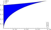
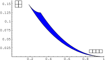
Figure 2: Left: the image $\mathsf{f}^{k}(\Delta(d))$ for $d=3$, $k=3$, projected onto the coordinates $\rho_{(1^{3})}$ and $\rho_{(2,1)}$. The convex hull of $\mathsf{f}^{k}(\Delta(d))$ is a polytope (see Example IV.4). Right: the image $\mathsf{f}^{k}(\Delta(d))$ for $d=3$, $k=4$ projected onto $\rho_{(4)}$ and $\rho_{(2,2)}$. The convex hull of this figure is not a polytope; since it is equal to the projection of the convex hull of $\mathsf{f}^{k}(\Delta(d))$, the latter set, $\mathcal{P}^{4}\cap\mathcal{W}^{4}$, cannot be a polytope.

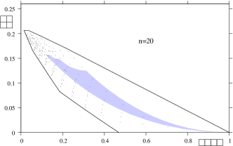
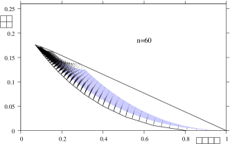
Figure 3: The figures show the image $\mathsf{f}^{k}(\Delta(d))$ (shaded region) for $d=5$, $k=4$, projected onto the coordinates $\rho_{(4)}$ and $\rho_{(2,2)}$. The image has a smooth convex boundary, so $\mathcal{P}^{4}\cap\mathcal{W}^{4}$ cannot be a polytope. Also shown are the points obtained by tracing out $n-k$ systems from states in $\mathcal{W}^{n}$. Each point corresponds to a diagram with $n=10$ boxes (top figure), $n=20$ (centre figure) and $n=60$ boxes (bottom figure); the line segments demarcate the convex hull of all the points. As expected, $\mathsf{f}^{k}(\Delta(d))$ is approximated more closely as $n$ increases.

V Conclusions

Although the quantum de Finetti theorem is usually thought of as a theorem about symmetric states, the unitary group shares the limelight in the results described here. Our highest weight version of the de Finetti theorem (Theorem II.2) generalises the usual symmetric-state version, but the extra generality almost comes free; indeed, one could argue that the structure of the proof is made clearer by taking the broader viewpoint. One can regard a highest weight vector as the state in a representation that is as unentangled as possible; this point of view has been taken by Klyachko Klyachko02 . It is therefore natural to regard highest weight vectors as analogues of product states, which is the role they have in our theorem.

In the special case of symmetric states, our Theorem II.7 gives bounds for the distance between the $n$-exchangeable state $\rho^{k}$ and the set $\mathcal{P}^{k}$ of convex combinations of products $\sigma^{\otimes k}$; these bounds are optimal in their dependence on $n$ and $k$, the theorem giving an upper bound of order $k/n$ and there being examples of states that achieve this bound (see Theorem II.10). The dependence of the bound on the dimension $d$ is less clear, the theorem giving a factor of $d^{2}$ whereas in the classical case Diaconis and Freedman DiaFre80 obtained a bound with a dimension factor of order $d$.

Diaconis and Freedman also obtained a bound, $\frac{k(k-1)}{2n}$, that is independent of the dimension. No such bound can exist for quantum states, as Example II.9 shows; one can find a state $\rho^{n}$ with the property that $\rho^{2}$, obtained by tracing out all but two of the systems, lies at a distance at least ${1}/{2}$ from $\mathcal{P}^{2}$. This example is a Werner state, in fact the fully antisymmetric state on $d=n$ systems, and it is an illustration of the usefulness of this family of states in giving information about $\mathcal{P}^{k}$.

Lemma III.6 shows that the shifted Schur functions OkoOls96 are closely connected with partial traces of Werner states. The meaning of this connection needs to be further explored: does the algebra of shifted symmetric functions have a quantum-informational significance?

Another intriguing connection is with the theorem of Keyl and Werner KeyWer01PRA . They show that the spectrum of a state $\rho$ can be measured by carrying out a von Neumann measurement of $\rho^{\otimes n}$ on the subspaces $U_{\lambda}\otimes V_{\lambda}$ in the Schur-Weyl decomposition of $(\mathbb{C}^{d})^{\otimes n}$ (equation (10)); if $\lambda$ is obtained, then $\bar{\lambda}=(\frac{\lambda_{1}}{n},\ldots,\frac{\lambda_{d}}{n})$ approximates the spectrum of $\rho$. Our theorem tells us that $\rho^{k}=\mathsf{tr}_{n-k}\rho^{n}_{\lambda}$ can be approximated by the twirled product $\sigma^{\otimes k}$, where $\sigma$ has spectrum $\bar{\lambda}$. By the Keyl-Werner theorem, the state $\mathsf{tr}_{n-k}\rho^{n}_{\lambda}$ must therefore project predominantly into subspaces $U_{\mu}\otimes V_{\mu}$ with $\mu$ close to $\lambda$ in shape (but rescaled by $k/n$). In this sense, tracing out a Werner state approximately ‘preserves the shape’ of its diagram. We can get an intuition for why this should be by iterating the special case of Lemma III.4 where one box is removed (cf. (Audenaert04, , Proposition 4)). This shows that tracing out is approximately equivalent, for large $n$, to a process that selects a row of a diagram with probability proportional to the length of that row and then removes a box from the end of the row.

There have been many applications of the de Finetti theorem to topics including foundational issues fuchsschacksecond ; Hudson81 , mathematical physics fannes ; raggiowerner and quantum information theory Ren05 ; bruncavesschack ; dohertyetal ; audenart ; terhaldoherty ; Ioannou06 ; there have also been various generalisations DiaFre80 ; HudMoo76 ; stormer ; fannesetal ; raggiowerner ; petz ; cavesfuchsschack ; fuchsschacksecond ; KoeRen05 ; Ren05 . We have taken one-and-a-half footsteps along this route.

- (1) A. Okounkov and G. Olshanski, (1996), q-alg/9605042.
- (2) B. de Finetti, Ann. Inst. H. Poincaré 7, 1 (1937).
- (3) E. Størmer, J. Funct. Anal. 3, 48 (1969).
- (4) R. L. Hudson and G. R. Moody, Z. Wahrschein. verw. Geb. 33, 343 (1976).
- (5) D. Petz, Prob. Th. Rel. Fields. 85 (1990).
- (6) C. M. Caves, C. A. Fuchs, and R. Schack, J. Math. Phys. 43, 4537 (2002), quant-ph/0104088.
- (7) C. A. Fuchs and R. Schack, (2004), quant-ph/0404156.
- (8) C. A. Fuchs, R. Schack, and P. F. Scudo, Phys. Rev. A 69, 062305 (2004), quant-ph/0307198.
- (9) R. König and R. Renner, J. Math. Phys. 46, 122108 (2005).
- (10) R. Renner, Security of Quantum Key Distribution, PhD thesis, ETH Zurich, 2005, quant-ph/0512258.
- (11) R. F. Werner, Phys. Rev. A 40, 4277 (1989).
- (12) R. Carter, G. Segal, and I. MacDonald, Lectures on Lie Groups and Lie Algebras, London Mathematical Society Student Texts Vol. 32, 1 ed. (cup, 1995).
- (13) A. Perelomov, Generalized coherent states and their applicationTexts and Monographs in Physics (Springer-Verlag, Berlin, 1986).
- (14) H. Weyl, The Theory of Groups and Quantum Mechanics (Dover Publications, Inc., New York, 1950).
- (15) P. Diaconis and D. Freedman, The Annals of Probability 8, 745 (1980).
- (16) M. Fannes, J. T. Lewis, and A. Verbeure, Lett. Math. Phys. 15, 255 (1988).
- (17) G. A. Raggio and R. F. Werner, Helv. Phys. Acta 62, 980 (1989).
- (18) L. M. Ioannou, Deterministic computational complexity of the quantum separability problem, quant-ph/0603199; to appear in QIP, 2006.
- (19) A. Doherty, personal communication, 2006.
- (20) K. Audenaert, (2004), available at http://qols.ph.ic.ac.uk/~kauden/QITNotes_files/irreps.pdf.
- (21) W. F. Fulton, Young Tableaux (Cambridge University Press, 1997).
- (22) T. Eggeling and R. F. Werner, Phys. Rev. A 63 (2000).
- (23) I. G. Macdonald, Symmetric functions and Hall polynomials (Clarendon Press, Oxford, 1979).
- (24) A. Klyachko, (2002), quant-ph/0206012.
- (25) M. Keyl and R. F. Werner, Phys. Rev. A 64, 052311 (2001).
- (26) R. L. Hudson, Found. Phys. 11, 805 (1981).
- (27) M. Fannes, H. Spohn, and A. Verbeure, J. Math. Phys. 21, 355 (1980).
- (28) T. A. Brun, C. M. Caves, and R. Schack, Phys. Rev. A 63, 042309 (2001).
- (29) A. C. Doherty, P. A. Parillo, and F. M. Spedalieri, Phys. Rev. A 69, 022308 (2004).
- (30) K. M. R. Audenaert, Proceedings of MTNS2004 (2004), quant-ph/0402076.
- (31) B. M. Terhal, A. C. Doherty, and D. Schwab, Phys. Rev. Lett 90, 157903 (2003).