Local aspects of disentanglement induced by spontaneous emission

Abstract

We consider spontaneous emission of two two-level atoms interacting with vacuum fluctuations. We study the process of disentanglement in this system and show the possibility of changing disentanglement time by local operations.

I Introduction

Creation of the entangled quantum states and its ability to transmit information is the base for quantum information NC . Recently, the subject has been intensively studied basically for two reasons. Firstly, the understanding of entanglement creation gives deep insight into the quantum mechanics foundations, and secondly, possible applications in quantum cryptography, quantum computing or teleportation of states are very promising. Hence, one of the main aims of such study is to get the knowledge about the complex nature of entanglement and its evolution in time.

In practice, every quantum system is open and susceptible to interaction with its environment. This may lead to the dissipation and destruction of correlations. Due to that, entanglement may disappear even though the system was initially in the entangled state. To control the process of disentanglement it is important to preserve as much entanglement as possible, because if entanglement once has been lost, it cannot be restored by local operations.

Spontaneous emission in two-atomic systems is an example of such noise which can diminish entanglementFT2 . On the other hand, due to the possible photon exchange between atoms, even in that case some separable initial states can evolve to entangled states JJ1 . In particular, when the interatomic distance is very small (compared with radiation wave length), the produced entanglement remains non-zero also for asymptotic states J .

In the present paper we study the simpler model of two atoms situated in independent thermostats at zero temperature. Since the atoms are separated by large distance, dipol - dipol interaction and photon exchange between atoms are negligible. Reduced dynamics of the system is given (in the Markovian approximation) by the semi - group of completely positive linear mappings A with generator $L$ parametrized only by the spontaneous emission rate of the single atom. In this model, the dynamics brings all initial states into unique asymptotic pure state, in which two atoms are in their ground states. Contrary to the infinite temperature case considered in JJ , where the neighbourhood of the asymptotic state contains only separable states, this asymptotic state lies on the boundary of the set of all states and there are separable as well as entangled states which are close to it. So there are initial entangled states which need only finite time to become separable during the evolution (they have finite disentanglement time), and on the other hand some initial states disentangle asymptotically (they have infinite disentanglement time).

The main goal of the present paper is to study local aspects of the process of disentanglement induced by spontaneous emission. We address the following question: what influence on the process of disentanglement can local operations performed on initial states have? As we show, local operations can change the robustness of initial entanglement against the noise, leading in some cases to enlarging the time needed to disentangle the state. In some classes of pure states, simple local operation can even change this time from finite to infinite. The same is true for Werner states. (Similar phenomenon was studied in E1 ).

We consider also non-local properties of quantum states which are manifested by violation of Bell - CHSH inequalities. As we show, during the evolution of the system initial states violating these inequalities become local after the finite time, even if disentanglement time is infinite.

II Spontaneous emission and evolution of entangled two-atomic systems

Let us consider two two-level atoms $A$ and $B$. Their excited states $|{1}\rangle_{A(B)}$ and ground states $|{0}\rangle_{A(B)}$ we identify with vectors $e_{1}=\left(\begin{array}[]{c}1\\ 0\\ \end{array}\right)$ and $e_{2}=\left(\begin{array}[]{c}0\\ 1\\ \end{array}\right)$ in $\mathbb{C}^{2}$. Since the atoms are separated by the long distance, it can be assumed that they are located inside two independent environments. The time evolution of density matrix of the considered system can be described by the master equation A :

$$\frac{d\varrho}{dt}=L\varrho\,=\,\,\frac{\Gamma_{AA}}{2}\,[\,\,2\,\sigma_{-}^{A}\,\varrho\,\sigma_{+}^{A}\,-\,\sigma_{+}^{A}\,\sigma_{-}^{A}\,\varrho\,-\,\varrho\,\sigma_{+}^{A}\,\sigma_{-}^{A}\,]+\,\frac{\Gamma_{BB}}{2}\,[\,\,2\,\sigma_{-}^{B}\,\varrho\,\sigma_{+}^{B}\,-\,\,\sigma_{+}^{B}\,\sigma_{-}^{B}\,\varrho\,-\,\varrho\,\sigma_{+}^{B}\,\sigma_{-}^{B}\,]$$ (II.1)

with definitions

$$\sigma_{\pm}^{A}=\sigma_{\pm}\otimes\mathbb{I},\quad\sigma_{\pm}^{B}=\mathbb{I}\otimes\sigma_{\pm},\quad\sigma_{3}^{A}=\sigma_{3}\otimes\mathbb{I},\quad\sigma_{3}^{B}=\mathbb{I}\otimes\sigma_{3},\quad\sigma_{\pm}=\frac{\displaystyle 1}{\displaystyle 2}\,(\sigma_{1}\pm\,i\sigma_{2})$$

In the following we consider two identical atoms, so $\Gamma_{AA}=\Gamma_{BB}=\Gamma_{0}$, where $\Gamma_{0}$ is the single atom sponatneous emission rate. Equation (II.1) can be used to obtain the equation of matrix elements of density matrix with respect to the basis $|1\rangle\otimes|1\rangle$,   $|1\rangle\otimes|0\rangle$,    $|0\rangle\otimes|1\rangle$,    $|0\rangle\otimes|0\rangle$

$$\rho_{11}(t) =e^{-2\Gamma_{0}t}\,\rho_{11}(0)$$ (II.2)

$$\rho_{12}(t) =e^{\frac{3}{2}\,\Gamma_{0}t}\,\rho_{12}(0)$$ (II.3)

$$\rho_{13}(t) =e^{\frac{3}{2}\,\Gamma_{0}t}\,\rho_{13}(0)$$ (II.4)

$$\rho_{14}(t) =e^{-\Gamma_{0}t}\,\rho_{14}(0)$$ (II.5)

$$\rho_{22}(t) =e^{-\Gamma_{0}t}\,(\rho_{22}(0)+\rho_{11}(0))-e^{-2\Gamma_{0}t}\,\rho_{11}(0)$$ (II.6)

$$\rho_{23}(t) =e^{-\Gamma_{0}t}\,\rho_{23}(0)$$ (II.7)

$$\rho_{24}(t) =e^{-\frac{1}{2}\,\Gamma_{0}t}\,(\rho_{13}(0)+\rho_{24}(0))-e^{-2\Gamma_{0}t}\,\rho_{13}(0)$$ (II.8)

$$\rho_{33}(t) =e^{-\,\Gamma_{0}t}\,(\rho_{33}(0)+\rho_{11}(0))-e^{-2\Gamma_{0}t}\,\rho_{11}(0)$$ (II.9)

$$\rho_{34}(t) =e^{-\frac{1}{2}\,\Gamma_{0}t}\,(\rho_{12}(0)+\rho_{34}(0))-e^{-\frac{3}{2}\,\Gamma_{0}t}\,\rho_{12}(0)$$ (II.10)

$$\rho_{44}(t) =1+\,e^{-2\Gamma_{0}t}\,\rho_{11}(0)-\,e^{-\Gamma_{0}t}\,(1-\rho_{44}(0)+\rho_{11}(0))$$ (II.11)

The remaining matrix elements can be obtained using the hermiticity condition $\rho_{kj}=\overline{\rho}_{jk}$. In this model the relaxation process brings all initial states to the unique asymptotic state when both atoms are in their ground states.

$$\rho_{\infty}=\begin{pmatrix}0&0&0&0\\ 0&0&0&0\\ 0&0&0&0\\ 0&0&0&1\end{pmatrix}$$ (II.12)

As a measure of the amount of entanglement of the given state of compound system $AB$, we take entanglement of formation Bennett which for for mixed states is given by

$$E\,(\,\rho\,)\,=\min\,\sum_{k}\,\lambda_{k}E\,(\,P_{k}\,),$$ (II.13)

where the minimum is taken over all possible decompositions

$$\rho\,=\,\sum_{k}\,\lambda_{k}\,P_{k}$$ (II.14)

In the special case of four-level systems, $E(\rho)$ is the function of another useful quantity $C(\rho)$ called concurrence, which we use here as a measure of entanglement HW ; Woo . The concurrence is defined as

$$C=\max\left(0,\,\sqrt{\lambda_{1}}-\sqrt{\lambda_{2}}-\sqrt{\lambda_{3}}-\sqrt{\lambda_{4}}\right)$$ (II.15)

where $\lambda_{i}$ are eigenvalues of the matrix

$$\hat{\rho}=(\,\rho^{\frac{1}{2}}\,\widetilde{\rho}\,\rho^{\frac{1}{2}}\,)^{\frac{1}{2}}$$ (II.16)

with $\widetilde{\rho}$ given by

$$\widetilde{\rho}=(\sigma_{2}\otimes\sigma_{2})\bar{\rho}(\sigma_{2}\otimes\sigma_{2})$$ (II.17)

where $\bar{\rho}$ is the complex conjugation of the matrix $\rho$. The range of concurrence is from 0 for separable states, to 1 for maximally entangled pure states.
In general concurrence is difficult to calculate analytically, so we consider the class of density matrices $\rho$

$$\rho=\begin{pmatrix}\rho_{11}&0&0&\rho_{14}\\ 0&\rho_{22}&\rho_{23}&0\\ 0&\rho_{23}&\rho_{33}&0\\ \rho_{41}&0&0&\rho_{44}\end{pmatrix}$$ (II.18)

One can check that the class of states given by (II.18) is invariant with respect to the time evolution considered in the paper, and

$$C(\rho)=\max\,\{\,0,\,C_{1},\,C_{2}\}$$ (II.19)

where

$$C_{1}=2(\,|\rho_{14}|-\sqrt{\rho_{22}\rho_{33}}\,)$$ (II.20)

$$C_{2}=2(\,|\rho_{23}|-\sqrt{\rho_{11}\rho_{44}}\,)$$ (II.21)

In particular when $\rho_{14}=0$ one can see that $C_{1}$ cannot be positive, so only $C_{2}$, if it is positive, contributes to the concurrence. Analogously when $\rho_{23}=0$ only $C_{1}$ can be considered.

Consider now the evolution of initial states (II.18). If $\rho_{14}=0$, then

$$\rho_{t}=\begin{pmatrix}\rho_{11}(t)&0&0&\rho_{14}(t)\\ 0&\rho_{22}(t)&0&0\\ 0&0&\rho_{33}(t)&0\\ \rho_{41}(t)&0&0&\rho_{44}(t)\end{pmatrix}$$ (II.22)

and

$$C(\rho_{t})=\max\,\{\,0,\,C_{1}(t)\}$$ (II.23)

where

$$C_{1}(t)=2e^{-\Gamma_{0}t}\left[|\rho_{14}|-\sqrt{e^{-2\Gamma_{0}t}\rho_{11}^{2}-e^{-\Gamma_{0}t}\rho_{11}(1-\rho_{44}+\rho_{11})+(\rho_{11}+\rho_{22})(\rho_{11}+\rho_{33})}\right]$$ (II.24)

In the equation (II.24), $\rho_{jk}$ denote matrix elements of the initial state.

On the other hand, if $\rho_{23}=0$, then

$$\rho_{t}=\begin{pmatrix}\rho_{11}(t)&0&0&0\\ 0&\rho_{22}(t)&\rho_{23}(t)&0\\ 0&\rho_{32}(t)&\rho_{33}(t)&0\\ 0&0&0&\rho_{44}(t)\end{pmatrix}$$ (II.25)

and

$$C(\rho_{t})=\max\,\{\,0,\,C_{2}(t)\}$$ (II.26)

where

$$C_{2}(t)=2e^{-\Gamma_{0}t}\left[|\rho_{23}|-\sqrt{1+e^{-2\Gamma_{0}t}\rho_{11}^{2}-e^{-\Gamma_{0}t}\rho_{11}(1+\rho_{11}-\rho_{44})}\right]$$ (II.27)

III Disentanglement time

In this section we study in details the time evolution of concurrence for some classes of initial states. Depending on the initial state, concurrence can reach value equal to zero asymptotically or at finite time. What is much more interesting, locally equivalent initial states with the same concurrence can disentangle at different times. It is even possible to change the time of disentanglement from finite to infinite. We show that this phenomenon happens for some classes of pure states and for Werner states.

III.1 Some pure initial states

Let

$$\phi=\frac{1}{\sqrt{2}}(\sqrt{1+\sqrt{1-C^{2}}},0,0,\sqrt{1-\sqrt{1-C^{2}}})$$ (III.1)

and $P_{\phi}$ be the corresponding projection operator

$$P_{\phi}=\frac{1}{2}\begin{pmatrix}1+\sqrt{1-C^{2}}&0&0&C\\ 0&0&0&0\\ 0&0&0&0\\ C&0&0&1-\sqrt{1-C^{2}}\end{pmatrix}$$ (III.2)

Then

$$P_{\phi}(t)=\begin{pmatrix}\tilde{c}e^{-2\Gamma_{0}t}&0&0&\frac{C}{2}e^{-\Gamma_{0}t}\\ 0&\tilde{c}(e^{-\Gamma_{0}t}-e^{-2\Gamma_{0}t})&0&0\\ 0&0&\tilde{c}(e^{-\Gamma_{0}t}-e^{-2\Gamma_{0}t})&0\\ \frac{C}{2}e^{-\Gamma_{0}t}&0&0&1-2\tilde{c}e^{-\Gamma_{0}t}+\tilde{c}e^{-2\Gamma_{0}t}\end{pmatrix}$$ (III.3)

where

$$\tilde{c}=\frac{1}{2}(1+\sqrt{1-C^{2}})$$ (III.4)

By (II.24) the time evolution of this initial concurrence C is described by the following function

$$C(P_{\phi}(t))=e^{-2\Gamma_{0}t}(1+\sqrt{1-C^{2}})-e^{-\Gamma_{0}t}(1+C+\sqrt{1-C^{2}})$$ (III.5)

We see that this function becomes equal to zero at time $t_{d}(\phi)$ (time of disentanglement), which is given by

$$t_{d}(\phi)=\frac{\ln(\frac{1}{2}(1+\sqrt{\frac{1+C}{1-C}}))}{\Gamma_{0}}$$ (III.6)

This time is finite for $C\in[0,1)$. When $C=1$ the states are maximally entangled and disentangle asymptotically. On the other hand, for locally equivalent pure states $\psi=(\sigma_{1}\otimes I_{2})\,\phi$:

$$\psi=\frac{1}{\sqrt{2}}(0,\sqrt{1+\sqrt{1-C^{2}}},\sqrt{1-\sqrt{1-C^{2}}},0)$$ (III.7)

with projection operator

$$P_{\psi}=\frac{1}{2}\begin{pmatrix}0&0&0&0\\ 0&1+\sqrt{1-C^{2}}&C&0\\ 0&C&1-\sqrt{1-C^{2}}&0\\ 0&0&0&0\end{pmatrix}$$ (III.8)

time evolution is given by

$$P_{\psi}(t)=\begin{pmatrix}0&0&0&0\\ 0&\frac{1}{2}(1+\sqrt{1-C^{2}})e^{-\Gamma_{0}t}&\frac{C}{2}e^{-\Gamma_{0}t}&0\\ 0&\frac{C}{2}e^{-\Gamma_{0}t}&\frac{1}{2}(1-\sqrt{1-C^{2}})e^{-\Gamma_{0}t}&0\\ 0&0&0&1-e^{-\Gamma_{0}t}\end{pmatrix}$$ (III.9)

and

$$C(P_{\psi}(t))=e^{-\Gamma_{0}t}C$$ (III.10)

We see that this function asymptotically goes to zero, so we can say that states (III.8) disentangle at infinite time. Thus we show that locally equivalent pure states with the same entanglement behave very differently during the time evolution and simple local unitary operation performed on initial state can change disentanglement time from finite to infinite.

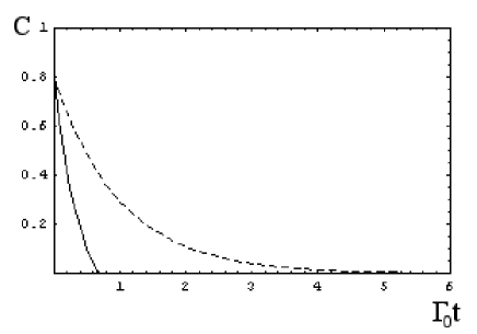
Figure 1: Concurrence as function of the time for initial state (III.8) (solid line) and (III.2) (dotted line) with $C=\frac{4}{5}$

III.2 Werner states

Similar phenomenon occurs for some mixed states. Consider the class of Werner states W

$$W_{\Psi_{\pm}}\,=\,(\,1\,-\,p\,)\,\frac{\mathbb{I}_{4}}{4}\,+\,p\,|\Psi_{\pm}\,\rangle\,\langle\,\Psi_{\pm}\,|,$$ (III.11)

$$W_{\Phi_{\pm}}\,=\,(\,1\,-\,p\,)\,\frac{\mathbb{I}_{4}}{4}\,+\,p\,|\Phi_{\pm}\,\rangle\,\langle\,\Phi_{\pm}\,|,$$ (III.12)

where $p\,\in\,[\,0,\,1\,]$ and $\,\Phi_{\pm}\,$,   $\Psi_{\pm}$ are maximally entangled pure Bell states defined as follows:

$$\Psi_{\pm}=\frac{1}{\sqrt{2}}\,[\,e_{1}\otimes e_{2}\pm e_{2}\otimes e_{1}\,],$$ (III.13)

and

$$\Phi_{\pm}=\frac{1}{\sqrt{2}}\,[\,e_{1}\otimes e_{1}\pm e_{2}\otimes e_{2}\,]$$ (III.14)

Since

$$W_{\Phi_{\pm}}(t)=\begin{pmatrix}\frac{1}{4}e^{-2\gamma\,\,t}(1+p)&0&0&\pm\frac{1}{2}e^{-\gamma\,\,t}p\\ 0&\frac{1}{2}e^{-\gamma\,\,t}-\frac{1}{4}e^{-2\gamma\,\,t}(1+p)&0&0\\ 0&0&\frac{1}{2}e^{-\gamma\,\,t}-\frac{1}{4}e^{-2\gamma\,\,t}(1+p)&0\\ \pm\frac{1}{2}e^{-\gamma\,\,t}p&0&0&1-\frac{1}{2}e^{-\gamma\,\,t}+\frac{1}{4}e^{-2\gamma\,t}(1+p)\end{pmatrix}$$ (III.15)

and

$$C(W_{\Phi_{\pm}}(t))=e^{-\Gamma_{0}t}p-\frac{1}{2}\left|e^{-2\Gamma_{0}t}(1+p)-2\right|$$ (III.16)

we see that

$$t_{d}(W_{\Phi_{\pm}})=\frac{\ln(\frac{1}{2}(\frac{1+p}{1-p}))}{\Gamma_{0}}$$ (III.17)

and this time is finite if $p\,\in\,[\,\frac{1}{3},\,1\,]$. On the other hand

$$W_{\Psi_{\pm}}(t)=\begin{pmatrix}\frac{1}{4}e^{-2\gamma\,\,t}(1-p)&0&0&0\\ 0&\frac{1}{2}e^{-\gamma\,\,t}-\frac{1}{4}e^{-2\gamma\,\,t}(1-p)&\pm\frac{1}{2}e^{-\gamma\,\,t}p&0\\ 0&\pm\frac{1}{2}e^{-\gamma\,\,t}p&\frac{1}{2}e^{-\gamma\,\,t}-\frac{1}{4}e^{-2\gamma\,\,t}(1-p)&0\\ 0&0&0&1-\frac{1}{2}e^{-\gamma\,\,t}+\frac{1}{4}e^{-2\gamma\,t}(1-p)\end{pmatrix}$$ (III.18)

and

$$C(W_{\Psi_{\pm}}(t))=e^{-\Gamma_{0}t}p-\frac{1}{2}e^{-\Gamma_{0}t}\sqrt{e^{-2\Gamma_{0}t}(1-p)^{2}-4(1-p)(1-e^{-\Gamma_{0}t})}$$ (III.19)

When $p\,\in\,[\,\frac{1}{3},\,\frac{-1+\sqrt{5}}{2}\,)$ this function is monotonically decreasing and reaches zero at time

$$t_{d}(W_{\Psi_{\pm}})=\frac{1}{\Gamma_{0}}\ln\frac{-1+p-\sqrt{(-1+p)^{2}p(1+p)}}{2(1-p-p^{2})}$$ (III.20)

But when $p\,\in\,[\,\frac{-1+\sqrt{5}}{2}\,,1],\;C(W_{\Psi_{\pm}}(t))$ goes to zero asymptotically, so we conclude that the disentanglement time is infinite.

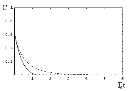
Figure 2: Concurrence as function of the time for initial state $W_{\Psi_{\pm}}$ (solid line) and $W_{\Phi_{\pm}}$ (dotted line) with $p=\frac{3}{4}$

Notice that

$$W_{\Phi_{+}}=(\mathbb{I}_{2}\otimes i\sigma_{2})\,W_{\Psi_{-}}(\mathbb{I}_{2}\otimes-i\sigma_{2}),\quad W_{\Phi_{-}}=(\mathbb{I}_{2}\otimes\sigma_{1})\,W_{\Psi_{-}}\,(\mathbb{I}_{2}\otimes\sigma_{1})$$

If $p\,\in\,[\,\frac{-1+\sqrt{5}}{2}\,,1]$ then the states $W_{\Phi_{\pm}}$ have the finite disentanglement time, whereas locally equivalent to them $W_{\Psi_{\pm}}$ disentangle asymptotically.

IV CHSH inequalities

Let us discuss now violation of Bell - CHSH inequalities by states evolving in time. It is known that all pure states violate Bell - CHSH inequalities whenever they are entangled. In the case of mixed states of two two-level systems, we can apply the following criterion HHH ; HH : Let

$$m(\rho)=\max_{j<k}\;(u_{j}+u_{k})$$ (IV.1)

where $u_{j},\,j=1,2,3$ are the eigenvalues of real symmetric matrix $U_{\rho}$ given by

$$U_{\rho}=T_{\rho}^{T}\,T_{\rho}$$ (IV.2)

with $T_{\rho}=(t_{nm})$,   $t_{nm}=\mathrm{tr}\,(\rho\,\sigma_{n}\otimes\sigma_{m})$. Than $\rho$ violates Bell - CHSH inequalities if and only if $m(\rho)\geq 1$. For the class (II.18)

$$m(\rho)=\max\left(\,u_{1},\,u_{2}\right)$$ (IV.3)

where

$$u_{1}=8(|\rho_{14}|^{2}+|\rho_{23}|^{2})$$ (IV.4)

and

$$u_{2}=4(|\rho_{14}|^{2}+|\rho_{23}|^{2})+\sqrt{(\rho_{23}+\rho_{32})^{2}(4|\rho_{14}|^{2}+(\rho_{23}-\rho_{32})^{2})}+(-1+2(\rho_{11}+\rho_{44}))^{2}$$ (IV.5)

Since interaction with environment destroys correlations, we expect that states which initially violate Bell - CHSH inequalities, during the evolution become local i.e. non-violating these inequalities. Consider for example pure initial states (III.2). One can check that

$$m(P_{\phi}(t))=\max\left(\,u_{1},\,u_{2}\right)$$ (IV.6)

where

$$u_{1}=2e^{-2\Gamma_{0}t}C^{2}$$ (IV.7)

and

$$u_{2}=e^{-2\Gamma_{0}t}C^{2}+(1-2e^{-\Gamma_{0}t})^{2}$$ (IV.8)

From the condition $m(\rho)=1$ we can calculate the locality time $t_{loc}$, after which Bell-CHSH inequalities are satisfied, and we obtain

$$t_{loc}=\left\{\begin{array}[]{ll}\frac{\ln(1+\frac{C^{2}}{4})}{\Gamma_{0}},&\qquad C\in[\,0,\,\,2(-1+\sqrt{2})]\\ \frac{\ln 2C^{2}}{2\Gamma_{0}},&\qquad C\in[\,2(-1+\sqrt{2})],\,\,1]\end{array}\right.$$ (IV.9)

For all $t\in[\,0,\,t_{loc}\,]$ the states $P_{\phi}(t)$ are entangled and violate Bell - CHSH inequalities.

On the other hand, in the case of initial states (III.8) this time is the same. We see that even if locally equivalent initial states disentangle at different times, the time after which they become local is the same. Similar calculations can be done for Werner initial states. Consider $p\,\in\,[\,\frac{1}{\sqrt{2}},\,1\,]$. Then initial states violate Bell - CHSH inequalities and

$$m(W_{\Psi_{\pm}}(t))=m(W_{\Phi_{\pm}}(t))=2e^{-2\Gamma_{0}t}p^{2}$$ (IV.10)

so

$$t_{loc}=\frac{\ln 2p^{2}}{2\Gamma_{0}}$$ (IV.11)

References

• (1) M.A. Nielsen, I.L. Chuang, Quantum Computation and Quantum Information, Cambridge University Press, Cambridge 2000.
• (2) R. TanaΕ›, Z. Ficek, J. Opt. B 6, S90(2004).
• (3) L. JakΓ³bczyk, A. JamrΓ³z, Phys. Lett. A 318, 318(2003).
• (4) L. JakΓ³bczyk, J. Phys. A 35, 6383(2002); J. Phys. A 36, 1573(2003), Corrigendum.
• (5) R.Alicki and K.Lendi K 1987 Quantum Dynamical Semigroups and Applications (Lecture Notes in Phys.vol 286) (Berlin: Springer).
• (6) L. JakΓ³bczyk, A. JamrΓ³z, Phys. Lett.A333, 35(2004).
• (7) Thing Yu, J.H.Eberly, Phys. Rev. Lett. 93, 140404(2004).
• (8) Ch. Bennett, P.D. DiVincenzo, J. Smolin, W.K. Wootters, Phys. Rev. A 54, 3824(1996).
• (9) S. Hill, W.K. Wooters, Phys. Rev. Lett. 78, 5022(1997).
• (10) W.K. Wooters, Phys. Rev. Lett. 80, 2254(1998).
• (11) R. Werner, Phys. Rev. A40, 4277(1989).
• (12) R. Horodecki, M. Horodecki, Phys. Rev. A 54, 1838(1996).
• (13) R. Horodecki, P. Horodecki, M. Horodecki, Phys. Lett. A 200, 340(1995).