Is there a prescribed parameter’s space for the adiabatic geometric phase?

Abstract. The Aharonov–Anandan and Berry phases are determined for the cyclic motions of a non–relativistic charged spinless particle evolving in the superposition of the fields produced by a Penning trap and a rotating magnetic field. Discussion about the selection of the parameter’s space and the relationship between the Berry phase and the symmetry of the binding potential is given.

PACS: 03.65 Ca, 03.65 Sq.

In 1984 Berry [1] discovered a geometric phase, which now is known as Berry’s or adiabatic phase and usually arises when an eigenstate of the Hamiltonian $H({\bf X}(t))$ evolves cyclically and adiabatically due to a cyclic and slow change of the parameters ${\bf X}(t)$. That phase was identified as a geometric property of the space of all possible values of ${\bf X}(t)$ (the parameter space) [2] and gave rise to the present interest on the geometric aspects of quantum theory [3–7]. An important generalization which does not need the adiabatic assumption (or equivalently that the initial state be an eigenstate of $H({\bf X}(t))$) was proposed by Aharonov and Anandan [3]. The essential requirement in the Aharanov–Anandan (AA) treatment is that the system performs a cyclic motion $|\psi(T)\rangle=e^{i\phi}|\psi(0)\rangle$, then the geometric phase is given by:

$$\beta=\phi+i\int_{0}^{T}\langle\psi(t)|{d\over{dt}}|\psi(t)\rangle dt.$$

$e^{i\beta}$ is the holonomy in the projective space of physical states, not a geometric property of the parameter space. However, as the adiabatic limit of the AA phase provides Berry phase (BP) this quantity can be considered also as a geometric property of the parameter space in this limit.

Recently, attention has been paid to the dynamics of systems interacting with magnetic fields and the determination of their cyclic motions [8–9]. For the situations involving a precessing magnetic field the AA phase and the BP have been calculated; in all these cases the BP turned out to be a linear function of $\cos\theta$, where $\theta$ is the semiangle of the cone swept by ${\bf B}(t)$ and is related to the solid angle by $\Delta\Omega=2\pi(1-\cos\theta)$. To the light of those results one might conclude that if a precessing magnetic field is involved in the cyclic evolution of a quantum system then the adiabatic phase will be simply a linear function of $\cos\theta$. This naive generalization is wrong because some facts must be taken into account. One of them is the ambiguity in choosing the parameter space when BP is evaluated according with the original Berry’s definition [1]. Because of the adiabatic nature of BP one could think that in its determination we only need to consider as forming the parameter space those quantities depending explicitly on time. However, in [1] the time–independent parameters were taken into account to achieve a geometric interpretation of BP (as the solid angle in the parameter space), but this is not a rule. For instance, if we consider a massive charged spherical oscillator with frequency $\omega_{0}$ interacting with ${\bf B}(t)$, the BP turns out proportional to $\cos\theta$ [9], then we don’t need to incorporate $\omega_{0}$ to the ${\bf B}(t)$–space. Other fact influencing on the BP is the symmetry of the binding potential. If we choose a binding potential with less symmetry than a spherical oscillator, the final BP will change, and this would lead us to conclude that the old parameter space (the ${\bf B}(t)$–space) must be modified in order to give a geometric interpretation of those results. These are the motivations for this paper, where we analize the geometric phases for a charged spinless particle evolving in the fields produced by a Penning trap with symmetry’s axis along the $x_{3}$–direction and simultaneously an orthogonally rotating magnetic field. The system is described by the Hamiltonian:

$$H(t)={1\over{2m}}\left({\bf p}+{e\over{2c}}{\bf r}\times{\bf B}(t)\right)^{2}+{m\over{2}}\omega_{0}^{2}\left(x_{3}^{2}-{{x_{1}^{2}+x_{2}^{2}}\over 2}\right),$$

where ${\bf B}(t)=(B\cos\omega t,B\sin\omega t,B_{0}),\ e<0$. In order to determine the cyclic motions, we first classify the system’s parameters according to the confined or unconfined nature induced by the Hamiltonian (2) on the quantum canonical trajectories. To simplify this classification, we take particular combinations of the parameters which for $B=0$ bring the evolution operator cyclically into the identity operator (the Penning loops [10], see also [11]). By restricting the parameters of the Penning loop and the rotating field to the confinement domain, we find the cyclic states of the system and evaluate their AA phases and BP. We discuss briefly the physical significance of these phases when the system is under the effect of an external periodic perturbation. Some remarks about the selection of the parameter space will be made. Finally we will compare graphically both the contributions to the BP of the three independent modes in which the system can be decomposed and $\cos\theta$. So, besides determining the geometric phases for a physically interesting system we give an evidence that the simple relationship between the BP and $\cos\theta$ for the systems previously studied is rather a consequence of the spherical symmetry possessed by the binding potential, which is lacking in the problem treated here.

The dynamics of a non–relativistic quantum system is governed by the Schrödinger’s equation, which in operator’s version reads ($\hbar=1$):

$${d\over{dt}}U(t)=-iH(t)U(t);\ \ \ \ \ U(0)=I.$$

If the Hamiltonian has the form (2), then the evolution operator $U(t)$ can be obtained by means of the “transition to the rotating frame” (see [12–14]), which maps (3) into a similar equation but with a time–independent Hamiltonian $G=H(0)-\omega L_{3}$. Hence, the solution of (3) has the disentangled form:

$$U(t)=e^{-i\omega tL_{3}}e^{-iGt}.$$

Note that $H(t)$ and $G$ are quadratic forms of the canonical 6–vector ${\bf u}^{\rm T}=({\bf r},{\bf p})$. Hence, the general motion’s properties of the system are determined by the kind of symplectic transformation induced by $e^{-iGt}$ on ${\bf u}$, ${\bf u}(t)=e^{iGt}{\bf u}e^{-iGt}=e^{\Lambda t}{\bf u}$, where $\Lambda$ is a $6\times 6$ matrix obtained of $[iG,{\bf u}]=\Lambda{\bf u}$ [12]. For the case in which $\Lambda$ is diagonalizable, we find two different behaviors, determined by the values taken by the three dimensionless parameters $\{\alpha={{|e|B}\over{2mc\omega}},\ \alpha_{0}={{|e|B_{0}}\over{2mc\omega}},\ w={{\omega_{0}}\over{\omega}}\}$. In one case all the six roots of the characteristic polynomial of $\Lambda$, $D(\lambda)=Det(\lambda I-\Lambda)$, are imaginary, and the spectral decomposition of the symplectic matrix $e^{\Lambda t}$ will induce confined motions on the canonical trajectories ${\bf u}(t)$. In the other case, at least two roots of $D(\lambda)$ have a non–null real part, and $e^{\Lambda t}$ will produce unconfined motions for ${\bf u}(t)$. The above two cases induce a similar classification on the $\alpha-\alpha_{0}-w$ space according to the roots of $D(\lambda)$ and, consequently, to the kind of generic motion possessed by the system at each point $(\alpha,\ \alpha_{0},\ w)$. For the sake of simplicity, we will restrict ourselves to physical situations in which, when $B=0$ the evolution operator (4) returns periodically into the identity operator (the Penning loops [10–11]). Moreover, we will take the simplest Penning loop which appears if we put $\omega_{0}={{2|e|B_{0}}\over{3mc}}$ ($w={4\over 3}\alpha_{0}$). With this choice, we have plotted the confinement and unconfinement regions in the $\alpha-\alpha_{0}$ diagram of Fig.1. The confinement domain consists of four disjoint regions, marked as $T_{i},i=1,\cdots,4$ and evaluated through a numerical calculation, while the unconfinement domain consists on the two remaining regions. Note that when $\alpha_{0}\rightarrow 0$ we recover the classification of the $\alpha$–line obtained in [12].

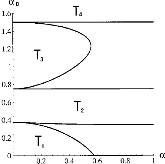
Figure 1: Classification of the $\alpha-\alpha_{0}$ plane according to the confined or unconfined canonical trajectories induced by $e^{\Lambda t}$ at each point $(\alpha,\alpha_{0})$ for a charged spinless particle evolving in the fields produced by the Penning loop with $w=4\alpha_{0}/3$ plus a rotating magnetic field. The confinement domain consists of the four disjoint regions $T_{i},i=1,\cdots,4$ while the remaining regions are the unconfinement domain.

Suppose the parameters $(\alpha,\alpha_{0})$ lie in some of the $T_{j}$–regions of Fig.1. Therefore, the eigenvalues of $\Lambda$ take the form $\{\pm i\omega_{1},\pm i\omega_{2},\pm i\omega_{3}\}$, and the Hamiltonian in the rotating frame can be decomposed as [9,12]:

$$G=\sum_{i=1}^{3}\epsilon_{i}\omega_{i}\left(A_{i}^{{\dagger}}A_{i}+{{\epsilon_{i}}\over 2}\right),$$

where $A_{i}^{{\dagger}},\ A_{i}$ are the ladder operators satisfying $[A_{i},A_{j}^{{\dagger}}]=\epsilon_{j}\delta_{ij}$, and $\epsilon_{i}=\pm 1$. Note that when $\epsilon_{i}=1$, the $A_{i}^{{\dagger}}$ and $A_{i}$ are equivalent to the standard creation and annihilation operators respectively, while when $\epsilon_{i}=-1$ the correspondence is in the inverted order. Expressions (4–5) suggest that the eigenstates of $G$, denoted by $|n_{1},n_{2},n_{3}\rangle$ and associated to the eigenvalues ${\cal E}_{n_{1}n_{2}n_{3}}$, form a natural base of bounded states of the system. Suppose that $|\psi(0)\rangle=|n_{1},n_{2},n_{3}\rangle$, then we can see that the state $|\psi(t)\rangle=U(t)|\psi(0)\rangle$ is cyclic with period $T=2\pi/\omega$:

$$|\psi(T)\rangle=e^{-i{\cal E}_{n_{1}n_{2}n_{3}}T}|\psi(0)\rangle.$$

A direct calculation (see Eq. (1)) shows that the geometric AA phase associated to this cyclic motion takes the form:

$$\beta_{n_{1}n_{2}n_{3}}=2\pi\langle n_{1},n_{2},n_{3}|L_{3}|n_{1},n_{2},n_{3}\rangle.$$

We can go a step further by expressing $\beta_{n_{1}n_{2}n_{3}}$ in terms of ${\cal E}_{n_{1}n_{2}n_{3}}$ [9]. A simple calculation provides:

$$\beta_{n_{1}n_{2}n_{3}}=-2\pi{\partial\over{\partial\omega}}{\cal E}_{n_{1}n_{2}n_{3}}=-2\pi\sum_{i=1}^{3}\epsilon_{i}\left(n_{i}+{1\over 2}\right){{\partial\omega_{i}}\over{\partial\omega}},$$

where $n_{i}\in{\bf Z}^{+},\ i=1,2,3$. It is important to remark that relations (7–8) are valid even if the precession of the magnetic field is fast. Relation (8) is the simplest generic form for the geometric phase when the evolution operator possesses the disentangled form (4).

It is interesting at this point to discuss how the geometric phases (8) influence on the physical properties of our system (for other kind of systems see for instance [15–17]). To this end, take (2) as an unperturbed Hamiltonian and add to it a small periodic perturbation of frequency $\omega_{p}$. It is known from time-dependent perturbation theory that when $\omega_{p}\simeq{\cal E}_{n_{1}n_{2}n_{3}}-{\cal E}_{n^{\prime}_{1}n^{\prime}_{2}n^{\prime}_{3}}$, where ${\cal E}_{n_{1}n_{2}n_{3}}={\cal E}_{n_{1}n_{2}n_{3}}(\omega)$, ${\cal E}_{n^{\prime}_{1}n^{\prime}_{2}n^{\prime}_{3}}={\cal E}_{n^{\prime}_{1}n^{\prime}_{2}n^{\prime}_{3}}(\omega)$, resonance phenomena will occur [15]. Suppose now that $\omega$ changes slightly by $\delta\omega$, i. e. $\omega\to\omega+\delta\omega$, then the unperturbed Hamiltonian (2) will be modified to $H(\omega+\delta\omega)$. Accordingly, in the perturbed case, the new resonance peak will become $\omega^{\prime}_{p}\simeq{\cal E}_{n_{1}n_{2}n_{3}}(\omega+\delta\omega)-{\cal E}_{n^{\prime}_{1}n^{\prime}_{2}n^{\prime}_{3}}(\omega+\delta\omega)$. Taking only the first two terms of the Taylor series of $\omega^{\prime}_{p}$ with respect to $\delta\omega$ we have $\omega^{\prime}_{p}\simeq\omega_{p}-{1\over 2\pi}(\beta_{n_{1}n_{2}n_{3}}-\beta_{n^{\prime}_{1}n^{\prime}_{2}n^{\prime}_{3}})\delta\omega$. As we can see, the resonance peak shifts by a quantity which depends only on the geometric phases of the two ”quasienergy” levels under consideration. In particular if $\omega\to 0$ the resonance peak shifting depends on the adiabatic (Berry) phase.

For calculational goals, we can express ${{\partial\omega_{i}}\over{\partial\omega}}$ in terms of $\omega_{i}$ itself. This last relation is more involved than (8) but it is useful when specific values of the parameters of the system are given and we want to evaluate the contribution of ${{\partial\omega_{i}}\over{\partial\omega}}$ to the geometric phase for each degree of freedom in which the original problem has been decomposed. We determined ${{\partial\omega_{i}}\over{\partial\omega}}$ for the adiabatic case using this technique and taking the limit $\omega\rightarrow 0$. We present the results in Fig.2, where in Fig. 2a we have plotted $\cos\theta=B_{0}(B_{0}^{2}+B^{2})^{-1/2}$, closely related to the solid angle in the ${\bf B}(t)$–space, as a function of the ratio $k\equiv B/B_{0}>0$; the contributions ${{\partial\omega_{i}}\over{\partial\omega}}_{|\omega=0},\ i=1,2,3$ as functions of $k$ are shown in Figs. 2b, 2c and 2d respectively. As we can see, $\cos\theta$ and ${{\partial\omega_{1}}\over{\partial\omega}}$ are well defined for all $k>0$ while ${{\partial\omega_{i}}\over{\partial\omega}},i=2,3$ are defined just in the interval $0<k<k_{cr}\approx 0.25831$. This is so because, unlike $\omega_{1}$, outside that $k$–interval the two degrees of freedom associated to $\omega_{2},\omega_{3}$ are not equivalent to the harmonic oscillator Hamiltonian. Therefore, those two degrees of freedom will produce unconfined motion on the canonical trajectories of our system. In that case there are not cyclic motions and so our relations to evaluate BP loose sense. Formulae (5–8) are valid for values of $k$ inside that interval, and because the three ${{\partial\omega_{i}}\over{\partial\omega}}$ cannot be just linear functions on $\cos\theta$, then the quadrupolar Penning potential affects them in a sensible way in contrast with a harmonic oscillator potential where they become proportional to $B_{0}(B_{0}^{2}+B^{2})^{-1/2}$. In the oscillator case the adiabatic phase is a function just on the parameters in the ${\bf B}(t)$– space, for this reason the dependence of BP on the spherical symmetry of the potential is not obvious. If, however, we choose a cylindrically symmetric potential (as the Penning trap potential of this work), the geometric phase will be a function on the binding parameters and, therefore, that dependence becomes apparent. So, in determining the BP for a bounded system we have to take into account both, the evolving parameters of the system and the symmetry of the binding potential which affects the BP through the eigenstates of the Hamiltonian.

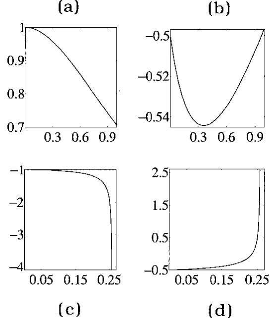
Figure 2: The relevant quantities for the Berry phase ${{\partial\omega_{i}}\over{\partial\omega}}_{|\omega=0},\ i=1,2,3$ as functions of $k=B/B_{0}$ are shown for two binding quadratic potentials having different symmetries. For a 3–dimensional oscillator (spherical symmetry) all three ${{\partial\omega_{i}}\over{\partial\omega}}_{|\omega=0},\ i=1,2,3$ are proportional to $\cos\theta=(1+k^{2})^{-1/2}$; in 2a we plot $\cos\theta$ versus $k$. For the Penning loop with $w=4\alpha_{0}/3$ (cylindrical symmetry) we display in 2b, 2c and 2d respectively the ${{\partial\omega_{i}}\over{\partial\omega}}_{|\omega=0},\ i=1,2,3$ as functions of $k$.

As an open question remains the possibility of finding a parameter’s space ${\bf X}(t)$ such that $\alpha({\bf X}(t))={\bf B}(t)$ with $\alpha$ being an automorphism of $R^{3}$, ${\bf X}(t)\in R^{3}$. It might be that in such a space the BP be again a linear function of $\cos\theta$.

To conclude, in this paper we have determined the confinement and unconfinement regions (see Fig.1) for the motion of a non–relativistic charged spinless particle evolving in the superposition of the fields produced by one of the Penning loops plus a rotating magnetic field. Working in the confinement domain we have calculated the AA phases and taking their adiabatic limit ($\omega\rightarrow 0$) the BP were obtained. We display graphically the differences between the relevant quantities for the BP associated to each degree of freedom in which the motion is decoupled and the corresponding ones obtained for a spherically symmetric binding potential. So, in Fig.2 the contrast between the two different symmetries is clearly shown, as might be expected for a quantity containing some of the geometric properties of the system.

D.J.F.C. acknowledges financial support from the Instituto de Cooperación Iberoamericana of the Agencia Española de Cooperación Internacional (Spain). N.B. acknowledges financial support from Dirección General de Investigación Científica y Técnica (Spain).

References

- [1] M.V. Berry, Proc. R. Soc. Lond. A 392, 45 (1984).
- [2] B. Simon, Phys. Rev. Lett. 51, 2167 (1983).
- [3] Y. Aharonov and J. Anandan, Phys. Rev. Lett. 58, 1593 (1987).
- [4] D.N. Page, Phys. Rev. A 36, 3479 (1987).
- [5] J. Anandan and Y. Aharonov, Phys. Rev. Lett. 65, 1697 (1990).
- [6] J. Anandan, in Quantum Coherence, J.A. Anandan Ed., World Scientific, Singapore (1990), p. 136.
- [7] L.J. Boya, J.F. Cariñena and J.M. Gracia–Bondía, Phys. Lett. A 161, 30 (1991).
- [8] D.J. Fernández C., L.M. Nieto, M.A. del Olmo and M. Santander, J. Phys. A 25, 5151 (1992).
- [9] D.J. Fernández C., M.A. del Olmo and M. Santander, J. Phys. A 25, 6409 (1992).
- [10] D.J. Fernández C., Nuovo Cim. B 107, 885 (1992).
- [11] B. Mielnik, J. Math. Phys. 27, 2290 (1986).
- [12] B. Mielnik and D.J. Fernández C., J. Math. Phys. 30, 537 (1989).
- [13] D.J. Moore and G.E. Stedman, J. Phys. A 23, 2049 (1990).
- [14] D.J. Moore, Phys. Rep. 210, 1 (1991).
- [15] Y. Wu and H. Li, Phys. Rev. B 38, 11907 (1988).
- [16] H.P. Breuer and M. Holthaus, Phys. Lett. A 140, 507 (1989).
- [17] M.V. Berry, Proc. R. Soc. Lond. A 430, 405 (1990).