Generation of bipartite spin entanglement via spin-independent scattering

Abstract

We consider the bipartite spin entanglement between two identical fermions generated in spin-independent scattering. We show how the spatial degrees of freedom act as ancillas for the creation of entanglement to a degree that depends on the scattering angle, $\theta$. The number of Slater determinants generated in the process is greater than 1, corresponding to genuine quantum correlations between the identical fermions. The maximal entanglement attainable of 1 e-bit is reached at $\theta=\pi/2$. We also analyze a simple $\theta$ dependent Bell’s inequality, which is violated for $\pi/4<\theta\leq\pi/2$. This phenomenon is unrelated to the symmetrization postulate but does not appear for unequal particles.

I Introduction

Bipartite and multipartite entanglement is the main resource that gives rise to many of the applications of quantum information and computation, like for example quantum teleportation Bennett et al. (1993); Bouwmeester et al. (1997) and quantum cryptography Wiesner (1983); Ekert (1991), among others (see for instance Refs. Nielsen and Chuang (2000); Galindo and Martín-Delgado (2002)). A compound system is entangled when it is impossible to attribute a complete set of properties to any of its parts. In this case, and for pure states, it is impossible to factor the state in a product of independent factors belonging to its parts. In this paper we will consider bipartite systems composed of two $s=\textstyle\frac{1}{2}$ fermions. Our aim is to uncover some specific features that apply when both particles are identical. They appear itemized in the next page.

States of two identical fermions have to obey the symmetrization postulate. This implies that they decompose into linear combinations of Slater determinants (SLs) of individual states. Naively, as these SLs cannot be factorized further, indistinguishability seems to imply entanglement. This is reinforced by the observation that the entropy of entanglement (EoE) is bounded from below by $S\geq 1$, well above the lower limit $S=0$ for a pair of non-entangled distinguishable particles. So, it looks like there is an inescapable amount of uncertainty, and hence of entanglement, in any state of two identical fermions. The above issue has been extensively examined in the literature Schliemann et al. (2001); Eckert et al. (2002); Ghirardi and Marinatto (2004) with the following result: Part of the uncertainty (giving $S=1$) corresponds to the impossibility to individuate which one is the first or the second particle of the system. This explains why the lower limit for the EoE is 1. Consider for instance two identical $s=\textstyle\frac{1}{2}$ fermions in a singlet state

$$\chi_{S}:=\frac{1}{\sqrt{2}}[\chi(1)^{\uparrow}\chi(2)^{\downarrow}-\chi(1)^{\downarrow}\chi(2)^{\uparrow}].$$

The antisymmetrization does not preclude the assignment of properties to the particles, but only assigning them precisely to particle 1 or particle 2. The reduced density matrix of any of the particles is $\rho=\frac{1}{2}\openone$ with an EoE $S(\rho)=1$. The portion of $S$ above 1 (if any) is genuine entanglement as it corresponds to the impossibility of attributing precise properties to the particles of the system Ghirardi and Marinatto (2004). Assume for instance that we endow the previous fermions with the capability of being outside ($\chi=\psi$) or inside ($\chi=\varphi$) the laboratory ($(\psi^{i},\psi^{j})=\delta^{ij}$, $(\varphi^{i},\varphi^{j})=\delta^{ij}$, $(\psi^{i},\varphi^{j})=0$, $i,j=\uparrow,\downarrow$). We now have two different possibilities: either the fermion outside has spin up ($\psi^{\uparrow}$) or spin down ($\psi^{\downarrow}$). Hence, there are two different SLs for a system built by a pair of particles with opposite spins, one outside, the other inside the laboratory

$${\rm SL}(1,2)_{1} = \frac{1}{\sqrt{2}}[\psi(1)^{\uparrow}\,\varphi(2)^{\downarrow}-\varphi(1)^{\downarrow}\,\psi(2)^{\uparrow}],$$

$${\rm SL}(1,2)_{2} = \frac{1}{\sqrt{2}}[\psi(1)^{\downarrow}\,\varphi(2)^{\uparrow}-\varphi(1)^{\uparrow}\,\psi(2)^{\downarrow}].$$ (1)

They form two different biorthogonal states, the combination $[{\rm SL}(1,2)_{1}-{\rm SL}(1,2)_{2}]/\sqrt{2}$ corresponding to the singlet and $[{\rm SL}(1,2)_{1}+{\rm SL}(1,2)_{2}]/\sqrt{2}$ to the triplet state (with respect to the total spin $\mathbf{s}=\mathbf{s}_{1}+\mathbf{s}_{2}$). An arbitrary state $\Phi(1,2)$ would then be a linear combination of these two SLs:

$$\Phi(1,2)\,=\,c_{1}{\rm SL}(1,2)_{1}\,+\,c_{2}{\rm SL}(1,2)_{2},\,\,\sum_{i}|c_{i}|^{2}=1,$$ (2)

giving an EoE

$$S\,=\,1-\sum_{i}|c_{i}|^{2}\,\log_{2}|c_{i}|^{2}\,\geq\,1.$$ (3)

Clearly, when $c_{1}$ or $c_{2}$ vanish, we come back to $S=1$, as the only uncertainty left is the very identity of the particles. Summarizing, while indistinguishability is an issue to be solved by antisymmetrization within each SL, entanglement is an issue pertaining to the superposition of different SLs Schliemann et al. (2001); Eckert et al. (2002); Ghirardi and Marinatto (2004). At the end, we could even decide to call 1 to the variables of the outside particle, and forget about symmetrization

$${\rm SL}(1,2)\rightarrow\,c_{1}\psi(1)^{\uparrow}\,\varphi(2)^{\downarrow}\,+\,c_{2}\psi(1)^{\downarrow}\,\varphi(2)^{\uparrow},$$ (4)

as both particles are far away from each other. In this case, the EoE $S=\,-\sum_{i}|c_{i}|^{2}\,\log_{2}|c_{i}|^{2}\geq 0$ is lesser than the one corresponding to antisymmetrized states by a quantity of 1, which is just the uncertainty associated to antisymmetrization. From now on we will consider the latter definition of $S$, which gives the genuine amount of entanglement between the two particles. Notice that for half-odd $s$, the number $\#{\rm{\rm SL}}$ of Slater determinants is bounded by $\#{\rm{\rm SL}}\leq(2s+1)d/2$, where $d$ is the dimension of each Hilbert space of the configuration or momentum degrees of freedom for each of the two fermions.

Much in the same way as above, we could consider one of the particles as right moving ($\chi=\psi_{0}$) the other as left moving ($\chi=\psi_{\pi}$), giving rise to two SLs in parallel with the above discussion. This is the first step towards the inclusion of the full set of commuting operators for the system. In addition to the spin components ($s_{1},s_{2}$) or helicities, there are the total $\mathbf{P}$ and relative $\mathbf{p}$ momenta. In the center of mass (CoM) frame we could consider the system described by the continuum of SLs

$${\rm SL}(1,2;\mathbf{p})_{s} = \frac{1}{\sqrt{2}}[\psi(1)_{0}^{s}\,\psi(2)_{\pi}^{-s}-\psi(1)_{\pi}^{-s}\,\psi(2)_{0}^{s}],$$

$${\rm SL}(1,2;\mathbf{p})_{-s} = \frac{1}{\sqrt{2}}[\psi(1)_{0}^{-s}\,\psi(2)_{\pi}^{s}-\psi(1)_{\pi}^{s}\,\psi(2)_{0}^{-s}],$$ (5)

where $\psi(1)_{0}^{s}=\langle 1|\mathbf{p}\,s\rangle$ and $\psi(1)_{\pi}^{s}=\langle 1|-\mathbf{p}\,s\rangle$. The labels 0 and $\pi$ are the azimuthal angles when we laid the axes along $\mathbf{p}$. Finally, there is a pair of SLs for each $\mathbf{p}$, so that a general state made with two opposite spin particles with relative momentum $\mathbf{p}$ could be written in the form:

$$\Phi(1,2)_{\mathbf{p}}^{0}\,=\,\sum_{s=\pm 1/2}\,c_{s}(\mathbf{p})\,{\rm SL}(1,2;\mathbf{p})_{s},$$ (6)

with $\sum_{s=\pm 1/2}\,|c_{s}(\mathbf{p})|^{2}=1$. Again, we run into the impossibility to tell which is 1 and which is 2. In addition there may be some uncertainty about the total spin state, whether a singlet or a triplet, or conversely, about the spin component of any of the particles, $\psi_{0}$ or $\psi_{\pi}$.

After this discussion it should be clear to what extent entanglement and distinguishability belong to different realms Schliemann et al. (2001); Eckert et al. (2002); Ghirardi and Marinatto (2004). The only requirement to include identical particles is to symmetrize the expressions used for unlike particles. Until now, we have only considered the free case. We have to examine the case of two interacting particles, as interaction is expected to be the source of subsequent entanglement Lamehi-Rachti and Mittig (1976); Törnqvist (1985); Pachos and Solano (2003); Manoukian and Yongram (2004); Aharonov et al. (2004); Saraga et al. (2004); Harshman (2005); Tal and Kurizki (2005); Lamata et al. (2006); Wang . Obviously, the answer may depend on a tricky way on the detailed form of the interaction, of its spin dependence in particular . It also seems that the role of particles identity, if any, will be played through symmetrization.

In the following we will show that spin entanglement is generated for the case of two interacting spin-$\textstyle\frac{1}{2}$ identical particles, with the following features:

• Spin-spin entanglement is generated even by spin independent interactions.

• In this case, it is independent of any symmetrization procedure.

• This phenomenon does not appear for unlike particles.

II Spin entanglement via spin-independent scattering

We first tackle the scattering of two unequal $s=\textstyle\frac{1}{2}$ particles $A$ and $B$ which run into each other with relative CoM momentum $\mathbf{p}$. We set the frame axes by the initial momentum $\mathbf{p}$ of particle $A$, and let the spin components be $s_{a}=s$ and $s_{b}=-s$ along an arbitrary but fixed axis. We will consider a spin independent Hamiltonian $H$, so the evolution conserves $\mathbf{s}_{a}$ and $\mathbf{s}_{b}$. We denote by $A_{\theta}^{s}$ $(B_{\theta}^{s})$ the state of particle $A$ ($B$) that propagates along direction $\theta$ with spin $s$. In these conditions the scattering proceeds as:

$$\Phi_{\mbox{in}}=\,A_{0}^{s}\,B_{\pi}^{-s}\longrightarrow\,\Phi_{\mbox{out}}(\theta)=\,f_{p}(\theta)\,A_{\theta}^{s}\,B_{\pi-\theta}^{-s},$$ (7)

where $\theta$ is the scattering angle and $f_{p}(\theta)$ the scattering amplitude. We will consider $\theta$ different from 0 or $\pi$ to avoid forward and backward directions. While the increase of uncertainty due to the interaction is clear, because a continuous manifold of final directions with probabilities $|f_{p}(\theta)|^{2}$ opened up from just one initial direction, spin remains untouched. The information about $s_{a}$ is the same before and after the scattering; as much as we knew the initial spin of $A$, we know its final spin whatever the final direction is. In other words, spin was not entangled by the interaction. We will now translate these well known facts to the case of identical particles, where they do not hold true.

Let particle $B$ be identical to $A$. Consider the same initial state as before: A particle $A$ with momentum $\mathbf{p}$ and spin $s$ runs into another $A$ with momentum $-\mathbf{p}$ and spin $-s$. Notice there is maximal information on the state. We could write $\Phi_{\mbox{in}}=\,A_{0}^{s}A_{\pi}^{-s}$, and eventually symmetrize. We now focus on the final state. It is no longer true that particle $A$ will come out with momentum $\mathbf{p^{\prime}}$ and spin $s$ with amplitude $f_{p}(\theta)$ while the amplitude for coming out with momentum $\mathbf{p^{\prime}}$ and spin $-s$ vanishes. Recalling that $B$ above did become $A$, the two cases $f_{p}(\theta)A_{\theta}^{s}B_{\pi-\theta}^{-s}$ and $f_{p}(\pi-\theta)A_{\pi-\theta}^{s}B_{\theta}^{-s}$ fuse into a unique state

$$\Phi_{\mbox{out}}(\theta)=f_{p}(\theta)\,A_{\theta}^{s}\,A_{\pi-\theta}^{-s}+f_{p}(\pi-\theta)\,A_{\pi-\theta}^{s}\,A_{\theta}^{-s},$$ (8)

as shown in Figure 1.

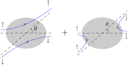
Figure 1: (Color online) Schematic picture of the two channels that contribute to the spin-independent scattering of two identical fermions. The shaded regions denote an arbitrary spin-independent interaction between the two fermions. The vertical arrows $\uparrow$, $\downarrow$ indicate the corresponding third component of spin.

Notice the uncertainty acquired by the spin: Now particle $A$ comes out from the interaction along $\theta$ either with spin $s$ or with spin $-s$, with relative amplitudes $f_{p}(\theta)$ and $f_{p}(\pi-\theta)$ respectively. In other words, spin was entangled during the spin independent evolution. Here, it is not the spin dependence of the interaction, but the existence of additional degrees of freedom which generate spin-spin entanglement. These, act as ancillas creating an effective spin-spin interaction that entangles the two fermions. The ancilla and the degree of entanglement depend on the scattering angle $\theta$. Notice that for $\theta=\pi/2$ both amplitudes $f_{p}(\theta)$ and $f_{p}(\pi-\theta)$ become equal, so that the degree of generated entanglement is maximal, 1 e-bit. On the other hand, for $\theta\simeq 0$, it generally holds $f_{p}(\theta)\gg f_{p}(\pi-\theta)$, so that in the forward and backward scattering almost no entanglement would be generated. However, this depends on the specific interaction. In Sec. III we will clarify this point with Coulomb interaction.

Symmetrization does not change this, it only expresses that we can not tell which one is 1 and which one is 2. The properly symmetrized initial state is

$$\Phi_{\mbox{in}} = {\rm SL}(1,2;\mathbf{p})_{s}$$ (9)

$$= \frac{1}{\sqrt{2}}[A(1)_{0}^{s}A(2)_{\pi}^{-s}-A(1)_{\pi}^{-s}A(2)_{0}^{s}].$$

The scattering process could be written in terms of SLs as

$${\rm SL}(1,2;\mathbf{p})_{s}\longrightarrow$$

$$f_{p}(\theta)\,{\rm SL}(1,2;\mathbf{p}^{\prime})_{s}-f_{p}(\pi-\theta)\,{\rm SL}(1,2;\mathbf{p}^{\prime})_{-s},$$ (10)

where $\mathbf{p}^{\prime}$ is the final momentum and the Slater determinants are given in (5). Both, this expression and Eq.(8), describe the same physical situation and lead to the same entanglement generation.

The bosonic case may be analyzed in an analogous way. The modification for two-dimensional spin Hilbert spaces (i.e. photons) would be a sign change in Eqs. (5), (9) and (10), as bosonic statistics has associated symmetric states. The equivalent of Eq. (10) for bosons is a genuine entangled state for $\theta\neq 0,\pi$, much as in the fermionic case.

III A specific example: Coulomb scattering at lowest order

We now consider Coulomb interaction at lowest order to illustrate the reasonings presented above. In this case

$$f_{p}(\theta) = \frac{N(e)}{t(\theta)},$$

$$f_{p}(\pi-\theta) = \frac{N(e)}{u(\theta)},$$ (11)

where $N(e)$ is a numerical factor depending on the charge $e$. $t(\theta)$ and $u(\theta)$ are two of the Mandelstam variables, associated to $t$ and $u$ channels respectively, and depending on the scattering angle $\theta$. for initial $p$ and final $p^{\prime}$ relative 4-momenta of the scattering fermions, they are given by $t=(p-p^{\prime})^{2}$, $u=(p+p^{\prime})^{2}$. In the CoM frame,

$$t(\theta)\!\! := 2(m^{2}-E^{2})(1-\cos\theta),$$

$$u(\theta)\!\! := 2(m^{2}-E^{2})(1+\cos\theta),$$ (12)

where $m$ is the mass of each fermion and $2E$ is the available energy.

According to this, the spin part of the state (8) for this case, properly normalized, is

$$|\chi_{\theta}\rangle=f_{+}(\theta)|\!\!\uparrow\downarrow\rangle-f_{-}(\theta)|\!\!\downarrow\uparrow\rangle,$$ (13)

being

$$f_{\pm}(\theta):=\frac{1\pm\cos\theta}{\sqrt{2(1+\cos^{2}\theta)}}.$$ (14)

The two amplitudes $f_{+}$ and $f_{-}$ vary monotonously as $\theta$ grows, becoming equal for $\theta=\pi/2$. The physical meaning for this is that for $\theta\rightarrow 0$, the knowledge about the system is maximal and the entanglement minimal (zero), and for increasing $\theta$ the knowledge of the system decreases continuously until reaching its minimum value at $\theta=\pi/2$. Accordingly, the entanglement grows with $\theta$ until reaching its maximum value for $\theta=\pi/2$.

We plot in Figure 2 the EoE Tal and Kurizki (2005) $S(\theta)=-f_{+}(\theta)^{2}\log_{2}f_{+}(\theta)^{2}-f_{-}(\theta)^{2}\log_{2}f_{-}(\theta)^{2}$ of state (13) as a function of $\theta$, for $0<\theta\leq\pi/2$. The entanglement grows monotonically until $\theta=\pi/2$, where it becomes maximal (1 e-bit).

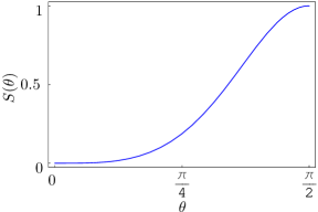
Figure 2: (Color online) EoE $S(\theta)$ as a function of $\theta$.

IV $\theta$-dependence of Bell’s inequality violation

In order to analyze the role the $\theta$ scattering angle plays in the generation of these genuine quantum correlations, we consider now the degree of violation of Bell’s inequality as a function of $\theta$. To this purpose, we define Bell (1964); Clauser and Shimony (1978) the observable

$$E(\mathbf{\hat{a}},\mathbf{\hat{b}}) := \langle\Phi|(\mathbf{\sigma}^{(1)}\cdot\mathbf{\hat{a}}\otimes\mathbf{\sigma}^{(2)}\cdot\mathbf{\hat{b}})|\Phi\rangle$$

$$= -[\hat{a}_{z}\hat{b}_{z}+2f_{p}(\theta)f_{p}(\pi-\theta)(\hat{a}_{x}\hat{b}_{x}+\hat{a}_{y}\hat{b}_{y})],$$

where $|\Phi\rangle:=|\Phi_{\rm out}(\theta)\rangle$ is the (normalized) state (8) and $\mathbf{\hat{a}}$, $\mathbf{\hat{b}}$ are arbitrary unit vectors. In Eq. (IV) we consider the amplitudes $f_{p}(\theta)$ and $f_{p}(\pi-\theta)$ normalized for each $\theta$, in the form $|f_{p}(\theta)|^{2}+|f_{p}(\pi-\theta)|^{2}=1$. We consider three coplanar unit vectors, $\mathbf{\hat{a}}$, $\mathbf{\hat{b}}$ and $\mathbf{\hat{c}}$. $(\widehat{\mathbf{\hat{a}},\mathbf{\hat{b}}})=\pi/3$, $(\widehat{\mathbf{\hat{a}},\mathbf{\hat{c}}})=2\pi/3$ and $(\widehat{\mathbf{\hat{b}},\mathbf{\hat{c}}})=\pi/3$. We have

$$|E(\mathbf{\hat{a}},\mathbf{\hat{b}})-E(\mathbf{\hat{a}},\mathbf{\hat{c}})|=1,$$

$$F(\theta):=1+E(\mathbf{\hat{b}},\mathbf{\hat{c}})=\frac{5}{4}-\frac{3}{2}f_{p}(\theta)f_{p}(\pi-\theta).$$ (16)

The Bell’s inequality, given by Bell (1964); Clauser and Shimony (1978)

$$|E(\mathbf{\hat{a}},\mathbf{\hat{b}})-E(\mathbf{\hat{a}},\mathbf{\hat{c}})|\leq 1+E(\mathbf{\hat{b}},\mathbf{\hat{c}}),$$ (17)

will then be

$$F(\theta)\geq 1.$$ (18)

For the particular case of Coulomb interaction at lowest order here considered, $2f_{p}(\theta)f_{p}(\pi-\theta)=2f_{+}(\theta)f_{-}(\theta)=(1-\cos^{2}\theta)/(1+\cos^{2}\theta)$ and thus the critical angle for which the inequality becomes violated is $\theta_{c}=\pi/4$ for $F(\theta_{c})=1$. For $\theta_{c}<\theta\leq\pi/2$ the Bell’s inequality does not hold. We show in Figure 3 the $\theta$ dependence of $F(\theta)$ together with the classical-quantum border, $F=1$, at $\theta_{c}=\pi/4$. Thus, for experiments with $\theta>\pi/4$ one could be able in principle to discriminate between local realism and quantum mechanics.

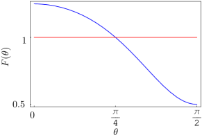
Figure 3: (Color online) $F(\theta)$ as a function of $\theta$. The classical-quantum border corresponds to $F(\theta_{c})=1$, with $\theta_{c}=\pi/4$.

This is in contrast with recent analysis of Bell’s inequalities violation in elementary particle systems Go (2004); Bramon et al. (2005); Törnqvist (1986), where the emphasis was placed on flavor entanglement, $K^{0}\bar{K}^{0}$, $B^{0}\bar{B}^{0}$, and the like. These analysis presented Bertlmann et al. (2004) two kinds of drawbacks coming from the lack of experimenter’s free will and from the unitary evolution with decaying states. These issues reduce the significance of the experiments up to the point of preventing their use as tests of quantum mechanics versus local realistic theories. The spin-spin entanglement analyzed in this paper does not have this kind of problems and could be used in principle for that purpose.

V Conclusions

In summary, we analyzed the relation between entanglement and antisymmetrization for identical particles, in the context of spin-independent particle scattering. We showed that, in order to create genuine spin-spin quantum correlations between two $s=\textstyle\frac{1}{2}$ fermions, spin-dependent interactions are not compulsory. The identity of the particles along with an interaction between degrees of freedom different from the spin, suffice for this purpose. The entanglement generated this way is not a fictitious one due to antisymmetrization, but a real one, and violates a certain Bell’s inequality for $\theta>\theta_{c}=\pi/4$.

References

- Bennett et al. (1993) C. H. Bennett, G. Brassard, C. Crépeau, R. Jozsa, A. Peres, and W. K. Wootters, Phys. Rev. Lett. 70, 1895 (1993).
- Bouwmeester et al. (1997) D. Bouwmeester, J. W. Pan, K. Mattle, M. Eibl, H. Weinfurter, and A. Zeilinger, Nature 390(6660), 575 (1997).
- Wiesner (1983) S. Wiesner, SIGACT News 15, 77 (1983).
- Ekert (1991) A. K. Ekert, Phys. Rev. Lett. 67, 661 (1991).
- Nielsen and Chuang (2000) M. A. Nielsen and I. L. Chuang, Quantum Computation and Quantum Information (Cambridge University Press, Cambridge, 2000).
- Galindo and Martín-Delgado (2002) A. Galindo and M. A. Martín-Delgado, Rev. Mod. Phys. 74, 347 (2002).
- Schliemann et al. (2001) J. Schliemann, J. I. Cirac, M. Kuś, M. Lewenstein, and D. Loss, Phys. Rev. A 64, 022303 (2001).
- Eckert et al. (2002) K. Eckert, J. Schliemann, D. Bruß, and M. Lewenstein, Ann. Phys. 299, 88 (2002).
- Ghirardi and Marinatto (2004) G. C. Ghirardi and L. Marinatto, Fortschr. Phys. 52, 1045 (2004).
- Lamehi-Rachti and Mittig (1976) M. Lamehi-Rachti and W. Mittig, Phys. Rev. D 14, 2543 (1976).
- Törnqvist (1985) N. A. Törnqvist, Helsinki University preprint HU-TFT-85-59 (1985).
- Pachos and Solano (2003) J. Pachos and E. Solano, Quant. Inf. Comput. 3, 115 (2003).
- Manoukian and Yongram (2004) E. B. Manoukian and N. Yongram, Eur. Phys. J. D 31, 137 (2004).
- Aharonov et al. (2004) Y. Aharonov, J. Anandan, G. J. Maclay, and J. Suzuki, Phys. Rev. A 70, 052114 (2004).
- Saraga et al. (2004) D. S. Saraga, B. L. Altshuler, D. Loss, and R. M. Westervelt, Phys. Rev. Lett. 92, 246803 (2004).
- Harshman (2005) N. L. Harshman, Int. J. Mod. Phys. A 20, 6220 (2005).
- Tal and Kurizki (2005) A. Tal and G. Kurizki, Phys. Rev. Lett 94, 160503 (2005).
- Lamata et al. (2006) L. Lamata, J. León, and E. Solano, Phys. Rev. A 73, 012335 (2006).
- (19) H.-J. Wang, eprint quant-ph/0510016.
- Bell (1964) J. S. Bell, Physics 1, 195 (1964).
- Clauser and Shimony (1978) J. F. Clauser and A. Shimony, Rep. Prog. Phys. 41, 1881 (1978).
- Go (2004) A. Go, J. Mod. Opt. 51, 991 (2004).
- Bramon et al. (2005) A. Bramon, R. Escribano, and G. Garbarino, J. Mod. Opt. 52, 1681 (2005).
- Törnqvist (1986) N. A. Törnqvist, Phys. Lett. A 117, 1 (1986).
- Bertlmann et al. (2004) R. A. Bertlmann, A. Bramon, G. Garbarino, and B. C. Hiesmayr, Phys. Lett. A 332, 355 (2004).