Entangled-state cycles from conditional quantum evolution

Abstract

A system of cascaded qubits interacting via the oneway exchange of photons is studied. While for general operating conditions the system evolves to a superposition of Bell states (a dark state) in the long-time limit, under a particular resonance condition no steady state is reached within a finite time. We analyze the conditional quantum evolution (quantum trajectories) to characterize the asymptotic behavior under this resonance condition. A distinct bimodality is observed: for perfect qubit coupling, the system either evolves to a maximally entangled Bell state without emitting photons (the dark state), or executes a sustained entangled-state cycle—random switching between a pair of Bell states while emitting a continuous photon stream; for imperfect coupling, two entangled-state cycles coexist, between which a random selection is made from one quantum trajectory to another.

I Introduction

Quantum entanglement is a feature of quantum mechanics that has captured much recent interest due to its essential role in quantum information processing Nielson . It may be characterized and manipulated independently of its physical realization, and it obeys a set of conservation laws; as such, it is regarded and treated much like a physical resource.

It proves useful in making quantitative predictions to quantify entanglement.When one has complete information about a bipartite system—subsystems $A$ and $B$—the state of the system is pure and there exists a well established measure of entanglement—the entropy of entanglement, evaluated as the von Neumann entropy of the reduced density matrix,

$$E(|\phi\rangle_{AB})=\textrm{Tr}(\rho_{A}\log_{2}\rho_{A}),$$ (1)

with $\rho_{A}\equiv\textrm{Tr}_{B}(|\phi\rangle\langle\phi|_{AB})$. This measure is unity for the Bell states and is conserved under local operations and classical communication. Unfortunately, however, quantum systems in nature interact with their environment; states of practical concern are therefore mixed, in which case the quantification of entanglement becomes less clear.

Given an ensemble of pure states, $\{|\phi_{i}\rangle_{AB}\}$ with probabilities $\{p_{i}\}$, a natural generalization of $E(|\phi\rangle_{AB})$ is its weighted average $\sum_{i}p_{i}E(|\phi_{i}\rangle_{AB})$. A difficulty arises, though, when one considers that a given density operator may be decomposed in infinitely many ways, leading to infinitely many values for this average entanglement. The density operator for an equal mixture of Bell states $|\Phi^{\pm}\rangle=(|0\rangle_{A}|0\rangle_{B}\pm|1\rangle_{A}|1\rangle_{B})/\sqrt{2}$, for example, is identical to that for a mixture of $|0\rangle_{A}|0\rangle_{B}$ and $|1\rangle_{A}|1\rangle_{B}$, yet by the above measure the two decompositions have entanglement one and zero, respectively.

Various measures have been proposed to circumvent this problem, most of which evaluate a lower bound. One such measure, the entanglement of formation, $E_{F}(\rho)$ bennet1 , is defined as the minimal amount of entanglement required to form the density operator $\rho$, while the entanglement of distillation, $E_{D}(\rho)$ bennet2 , is the guaranteed amount of entanglement that can be extracted from $\rho$. These measures satisfy the requirements for a physical entanglement measure set out by Horodecki et al. horodecki3 . They give the value zero for $\rho_{AB}=(|\Phi^{+}\rangle\langle\Phi^{+}|+|\Phi^{-}\rangle\langle\Phi^{-}|)/2$, which might be thought somewhat counterintuitive, since this state can be viewed as representing a sequence of random “choices” between two Bell states, both of which are maximally entangled. This is unavoidable, however, because assigning $\rho_{AB}$ a non-zero value of entanglement would imply that entanglement can be generated by local operations. The problem is fundamental, steming from the inherent uncertainty surrounding a mixed state: the state provides an incomplete description of the physical system, and in view of the lack of knowledge a definitive measure of entanglement cannot be given.

An interacting system and environment inevitably become entangled. The problem of bipartite entanglement for an open system is therefore one of tripartite entanglement for the system and environment. Complicating the situation, the state of the environment is complex and unknown. Conventionally, the partial trace with respect to the environment is taken, yielding a mixed state for the bipartite system. If one wishes for a more complete characterization of the entanglement than provided by the above measures, somehow the inherent uncertainty of the mixed state description must be removed.

To this end, Nha and Carmichael Nha04a recently introduced a measure of entanglement for open systems based upon quantum trajectory unravelings of the open system dynamics Carmichael93 . Central to their approach is a consideration of the way in which information about the system is read, by making measurements, from the environment. The evolution of the system conditioned on the measurement record is followed, and the entanglement measure is then contextual—dependent upon the kind of measurements made. Suppose, for example, that at some time $t$ the system and environment are in the entangled state

$$|\phi\rangle=\sum_{i,j}c_{i,j}|\phi_{i}\rangle_{S}|\phi_{j}\rangle_{E}.$$ (2)

A partial trace with respect to $E$ yields a mixed state for $S$. If, on the other hand, an observer makes a measurement on the environment with respect to the basis $\{|\phi_{j}\rangle_{E}\}$, obtaining the “result” $|\phi_{k}\rangle_{E}$, the reduced state of the system and environment is

$$|\phi^{\prime}\rangle=|\phi^{\prime}\rangle_{S}|\phi_{k}\rangle_{E},$$ (3a)

with conditional system state

$$|\phi^{\prime}\rangle_{S}=\sum_{i}c_{i,k}|\phi_{i}\rangle_{S}/\sqrt{p_{k}},$$ (3b)

where $p_{k}=\sum_{i}|c_{i,k}|^{2}$ is the probability of the particular measurement result. Thus, the system and environment are disentangled, so the system state is pure and its bipartite entanglement is defined by the von Neumann entropy, Eq. (1). Nha and Carmichael Nha04a apply this idea to the continuous measurement limit, where $|\phi^{\prime}\rangle_{S}$ executes a conditional evolution over time.

In this paper we follow the lead of Nha and Carmichael, also Carvalho et al. Carvalho05 , not to compute their entanglement measure per se, but to examine the entanglement dynamics of a cascaded qubit system coupled through the oneway exchange of photons. The system considered has been shown to produce unconditional entangled states—generally a superposition of Bell states—as the steady-state solution to a master equation Clark03 . For a special choice of parameters (resonance), a maximally entangled Bell state is achieved $\ldots$ except that the approach to the steady state takes place over an infinite amount of time.

Here we analyze the conditional evolution of the qubit system to illuminate the dynamical creation of entanglement in the general case, and to explain, in particular, the infinitely slow approach to steady-state in the special case. We demonstrate that in the special case the conditional dynamics exhibit a distinct bimodality, where the approach to the Bell state is only one of two possibilities for the asymptotic evolution: the second we call an entangled-state cycle, where the qubits execute a sustained stochastic switching between two Bell states. Though involving just two qubits and elementary quantum transitions, the situation is similar to that of a bimodal system in classical statistical physics in the limit of a vanishing transition rate between attractors.

The physical model of the cascaded qubit system is presented in Sec. II and the quantum trajectory unraveling of its conditional dynamics in Sec. III. In Sec. IV we analyze the quantum trajectory equations to demonstrate bimodality and the existence of entangled-state cycles. Finally, a discussion and conclusions are presented in Sec. V.

II The Cascaded Qubit System

In this section we briefly outline the physical model for the cascaded qubit system to be analyzed. A more detailed description, together with the techniques and assumptions used to derive the model master equation presented here, is available in Clark03 .

II.1 Physical Configuration

The system considered consists of two high-finesse optical cavities, each containing a single tightly-confined atom, the cavities arranged in a cascaded configuration with unidirectional coupling from cavity 1 to cavity 2 (Fig. 1). For simplicity, we consider the cavity modes to be identical, with resonance frequency $\omega_{\rm cav}$ and field decay rate $\kappa$. Inefficiencies and losses in the coupling between the cavities are modeled by a real parameter $\epsilon$, $0\leq\epsilon\leq 1$, with perfect coupling corresponding to $\epsilon=1$. The atoms are assumed to have five relevant electronic levels, of which two ground states, $|0\rangle$ and $|1\rangle$, represent an effective two-state system, or qubit.

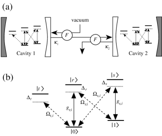
Figure 1: (a) A pair of cascaded cavities, Cavity 1 and Cavity 2, each contain a single trapped atom; a unidirectional coupling between the cavities is realized by Faraday isolators F. (b) The atomic excitation scheme couples two stable ground states, $|0\rangle$ and $|1\rangle$, to three excited states, $|r\rangle$, $|s\rangle$, and $|t\rangle$.

For each atom, the cavity field in combination with auxiliary laser fields (incident from the side of the cavity) drives two separate resonant Raman transitions between states $|0\rangle$ and $|1\rangle$. An additional laser field coupled to the $|0\rangle\leftrightarrow|t\rangle$ transition provides a tunable light shift of the energy of state $|0\rangle$. All fields are assumed far detuned from the atomic excited states, so these states may be adiabatically eliminated and atomic spontaneous emission ignored. Under the further assumption that the cavity field decay rate is much larger than the transition rates between $|0\rangle$ and $|1\rangle$, the cavity fields may also be adiabatically eliminated to yield a master equation for the reduced two-atom density matrix $\rho$,

$$\dot{\rho}=\mathcal{L}\rho = \sum_{i=1,2}\left(2\hat{R}_{i}\rho\hat{R}_{i}^{\dagger}-\hat{R}_{i}^{\dagger}\hat{R}_{i}\rho-\rho\hat{R}_{i}^{\dagger}\hat{R}_{i}\right)$$ (4)

$$-2\sqrt{\epsilon}\left(\left[\hat{R}_{1}\rho,\hat{R}_{2}^{\dagger}\right]+\left[\hat{R}_{2},\rho\hat{R}_{1}^{\dagger}\right]\right),$$

with

$$\hat{R}_{i}=(\beta_{r,i}\hat{\sigma}_{i-}+\beta_{s,i}\hat{\sigma}_{i+})/\sqrt{\kappa},$$ (5)

where $\sigma_{i-}\equiv(|0\rangle\langle 1|)_{i}$, and $|\beta_{r,i}|^{2}/\kappa$ and $|\beta_{s,i}|^{2}/\kappa$ are the rates of $|1\rangle_{i}\rightarrow|0\rangle_{i}$ and $|0\rangle_{i}\rightarrow|1\rangle_{i}$ transitions, respectively.

By virtue of the cavity output, the system is an open system and solutions to master equation (4) generally describe mixed states. Under appropriate conditions, however, the system evolves to a pure and entangled steady state.

II.2 Steady State

If the coupling between cavities is perfect ($\epsilon=1$) and the parameters of the subsystems are the same ($\beta_{r,1}=\beta_{r,2}=\beta_{r}$, $\beta_{s,1}=\beta_{s,2}=\beta_{s}$) then the steady state is the pure state

$$|\phi_{\rm ss}\rangle=\frac{1}{\sqrt{|\beta_{r}|^{2}+|\beta_{s}|^{2}}}\left(\beta_{r}^{*}|00\rangle+\beta_{s}^{*}|11\rangle\right),$$ (6)

where we use the abbreviated notation $|00\rangle\equiv|0\rangle_{1}|0\rangle_{2}$ and $|11\rangle\equiv|1\rangle_{1}|1\rangle_{2}$. Then when $\beta_{r}=\beta_{s}$, which we shall refer to as the resonance condition, the steady state is a maximally-entangled Bell state. This may seem to be ideal, but a problem arises when we consider the eigenvalues of the operator $\mathcal{L}$. Specifically, the characteristic time for the system to reach steady state, $\tau=\left|{\rm Re}(\lambda_{2})\right|^{-1}$, where $\lambda_{2}$ denotes the eigenvalue of $\mathcal{L}$ with smallest (in magnitude) non-zero real part, approaches infinity as the resonance condition is approached. This is shown by the plot in Fig. 2. Thus the master equation itself, in particular its steady state, offers limited insight into the behavior of the system at resonance. We wish to learn more about this special case; in particular, how does the entanglement develop dynamically. Also, if additional information is factored into the description, by making measurements on the environment, can we better characterize the long term behavior, or possibly find perfect entanglement after a finite time? We demonstrate that quantum trajectory theory can provide answers to these questions.

Figure 2: The relaxation time $\tau=|{\rm Re}(\lambda_{2})|^{-1}$ plotted as a function of $|\beta_{s}/\beta_{r}|$. Note the singularity at resonance, $|\beta_{s}/\beta_{r}|=1$.

III Quantum Trajectories

As with any open system, the first step in unraveling the master equation is to identify the points of coupling to the environment. The first is obvious – the output from Cavity 2. To measure this output, let us assume the existence of an ideal photon detector in the path of the output from Cavity 2; we call it Detector 1.

The second point of coupling to the environment is more subtle. Our model does not assume the inter-cavity coupling to be perfect; only a fraction $\epsilon$ of the output photon flux from Cavity 1 makes it into Cavity 2. Physically, this loss may be caused, for example, by non-ideal transmissivity of the Faraday isolators or by absorption in the cavity mirrors. These imperfections cause photons to be scattered into the environment in some uncontrollable fashion. Formally, though, this is equivalent to assuming that the apparatus is ideal, except that there exists a beamsplitter between the cavities, as drawn schematically in Fig. 3. We therefore further assume the existence of a second photon detector to collect photons reflected by this beamsplitter; we call it Detector 2.

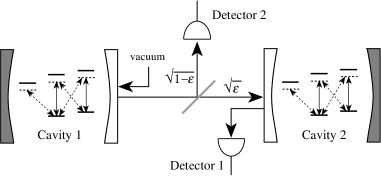
Figure 3: Conceptual photon detectors, Detector 1 and Detector 2, used for unravelling the master equation. The Faraday isolators are omitted for clarity.

We now proceed to develop the quantum trajectory formalism for the cascaded qubit system. In this approach the system is described by a pure state which is dependent on (conditioned on) the counting histories, or records, of Detectors 1 and 2. Firstly, we rewrite the master equation in a form suitable for translation into the quantum trajectory language. We reexpress Eq. (4) in the form

$$\dot{\rho} =(\mathcal{L}_{0}+\mathcal{S})\rho,$$ (7)

with

$$\mathcal{L}_{0}\rho \equiv-i\left[\hat{H}_{0},\rho\right]-\frac{1}{2}\sum_{i=1,2}\left(\hat{C}_{i}^{{\dagger}}\hat{C}_{i}\rho+\rho\hat{C}_{i}^{{\dagger}}\hat{C}_{i}\right),$$ (8a)

$$\mathcal{S}\rho =\sum_{i=1,2}\hat{C}_{i}\rho\hat{C}_{i}^{{\dagger}},$$ (8b)

where

$$\hat{C}_{1} = \sqrt{2}\left(\sqrt{\epsilon}\hat{R}_{1}-\hat{R}_{2}\right),$$ (9a)

$$\hat{C}_{2} = \sqrt{2(1-\epsilon)}\,\hat{R}_{1},$$ (9b)

$$\hat{H}_{0} = i\sqrt{\epsilon}\left(\hat{R}_{2}^{{\dagger}}\hat{R}_{1}-\hat{R}_{1}^{{\dagger}}\hat{R}_{2}\right).$$ (9c)

Then, within quantum trajectory theory, the evolution of the system is described by a pure state $|\phi\rangle$ which evolves under the non-Hermitian effective Hamiltonian

$$\hat{H}_{\rm eff}=\hat{H}_{0}-i\frac{1}{2}\sum_{i=1,2}\hat{C}_{i}^{{\dagger}}\hat{C}_{i},$$ (10)

the continuous evolution interrupted at random times by quantum jumps, $|\phi\rangle\rightarrow\hat{C}_{i}|\phi\rangle$, where the jumps occur with probability

$$p_{i}(t)dt=\frac{\langle\phi|\hat{C}_{i}^{{\dagger}}\hat{C}_{i}|\phi\rangle}{\langle\phi|\phi\rangle}dt$$ (11)

in time interval $(t,t+dt)$. Physically, the jump operators $\hat{C}_{1}$ and $\hat{C}_{2}$ account for the reduction of the state of the system, given a photon count is recorded by Detector 1 or Detector 2, respectively. Thus, within the quantum trajectory description of the coupled cavity system, we consider an experiment in which ideal detectors are employed, such that every scattered photon is detected and recorded. Given the history of detector ‘clicks’, one has complete information about the system state, in the sense that that state is always pure; hence, although the solution to the master equation is generally mixed, one is able to characterize the entanglement in an unambiguous (conditional) fashion Nha04a .

Consider the special case where the coupling between the cavities is optimal ($\epsilon=1$). In this case there is only one output from the system, that from Cavity 2, recorded by Detector 1. Standard numerical algorithms QOToolbox have been used to simulate typical quantum trajectories for various values of $|\beta_{s}/\beta_{r}|$. Specifically, we consider the evolution of the conditional expectation of the operator product $\hat{\sigma}_{1,z}\hat{\sigma}_{2,z}$, where $\hat{\sigma}_{i,z}$ is the Pauli operator diagonal in the $\left(|0\rangle_{i},|1\rangle_{i}\right)$–representation,

$$\hat{\sigma}_{i,z}|1\rangle_{i}=|1\rangle_{i},\qquad\hat{\sigma}_{i,z}|0\rangle_{i}=-|0\rangle_{i}\,.$$ (12)

This expectation has a number of convenient properties; for example, the steady-state value

$$\left\langle\hat{\sigma}_{1,z}\hat{\sigma}_{2,z}\right\rangle_{\rm ss}=1,$$ (13)

regardless of the value of $|\beta_{s}/\beta_{r}|$, which makes it easy to compare rates of convergence to the steady state for different system parameters.

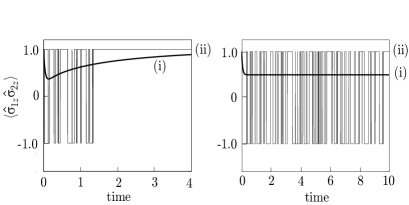
Figure 4: Evolution of the ensemble average (i) compared with that of a single quantum trajectory (ii), for $\epsilon=1$. The off-resonance case ($\beta_{s}\neq\beta_{r}$) is shown to the left and compared with the resonant case ($\beta_{s}=\beta_{r}$) to the right. Time is measured in units of $\left(\beta_{r}/\sqrt{\kappa}\right)^{-1}$.

Figure 4 contrasts the solution to the master equation and a single quantum trajectory. The solution to the master equation exhibits a completely smooth evolution that tends asymptotically towards the steady state. The quantum trajectory, on the other hand, undergoes a sequence of switches between two extreme values of $\left\langle\hat{\sigma}_{1,z}\hat{\sigma}_{2,z}\right\rangle$, which occur at each photon detection. Provided the parameters are chosen away from resonance, the photon detections eventually stop and the trajectory settles into the steady state (6), with $\left\langle\hat{\sigma}_{1,z}\hat{\sigma}_{2,z}\right\rangle=1$; the steady state is clearly a dark state. At resonance, however, the photon detections may continue indefinitely. Physically, this seems plausible, since it simply implies that the atoms continue to switch between states $|0\rangle$ and $|1\rangle$, scattering one photon with each transition. At resonance, apparently, a unique equilibrium dark state cannot be established. The cyclic behavior that replaces it is completely invisible if we consider only the ensemble average–a vivid demonstration of how single quantum trajectories can provide additional insight into the evolution of an open quantum system.

IV Entangled-state Cycles

The oscillatory behavior featured in Fig. 4 hints at a simple cyclic process. In fact, it is simple enough that we can understand why it occurs without resorting to numerics. In this section we formulate a graphical description of individual trajectories.

IV.1 The Cascaded System Phase Space

Figure 4 demonstrates that the conditional expectation $\left\langle\hat{\sigma}_{1,z}\hat{\sigma}_{2,z}\right\rangle$ is conserved during the periods of evolution between quantum jumps. The positively and negatively correlated subspaces

$$E^{\pm}=\left\{|\phi\rangle:\left\langle\hat{\sigma}_{1,z}\hat{\sigma}_{2,z}\right\rangle=\pm 1\right\}$$ (14)

are coupled only through quantum jumps. Noting that

$$E^{+}=\textrm{span}\{|00\rangle,|11\rangle\},\quad E^{-}=\textrm{span}\{|10\rangle,|01\rangle\}$$ (15)

are each $2$-dimensional (assuming real amplitudes without loss of generality), we manage to break up a $4$-dimensional space into two $2$-dimensional planes, linked to one another by the quantum jumps. We refer to this representation as the cascaded system phase space. Trajectories within it can be viewed as lines moving continuosly within either plane and jumping discontinuously between the planes.

IV.2 Evolution Between Quantum Jumps

We use phase space portraits within $E^{+}$ and $E^{-}$ to characterize the behavior of the system, where for the sake of simplicity, and without loss of generality, we are assuming $\beta_{r}$ and $\beta_{s}$ to be real. We define

$$r=|\beta_{s}/\beta_{r}|=\beta_{s}/\beta_{r},$$ (16)

and scale time by setting $\beta_{r}/\sqrt{\kappa}=1$. The master equation then takes the form ($\epsilon=1$)

$$\dot{\rho}= \sum_{i=1,2}\left(2\hat{R}_{i}\rho\hat{R}_{i}^{{\dagger}}-\hat{R}_{i}^{{\dagger}}\hat{R}_{i}\rho-\rho\hat{R}_{i}^{{\dagger}}\hat{R}_{i}\right)$$

$$+2(\rho\hat{R}_{1}^{{\dagger}}\hat{R}_{2}-\hat{R}_{2}\rho\hat{R}_{1}^{{\dagger}}+\hat{R}_{2}^{{\dagger}}\hat{R}_{1}\rho-\hat{R}_{1}\rho\hat{R}_{2}^{{\dagger}}),$$ (17)

where

$$\hat{R}_{i}=\hat{\sigma}_{i}^{-}+r\hat{\sigma}_{i}^{+}.$$ (18)

The resonance condition is now $r=1$.

It is useful to convert to a matrix notation, such that a pure state $|\phi\rangle$ of the system is represented by a $4$-vector,

$$|\phi\rangle=(c_{11},c_{10},c_{01},c_{00})^{T}\equiv\sum_{i,j=0,1}c_{ij}|ij\rangle\,,$$ (19)

and system operators are written as $4\times 4$ matrices, e.g.,

$$\hat{R}_{1}=\left(\begin{array}[]{cccc}0&0&r&0\\ 0&0&0&r\\ 1&0&0&0\\ 0&1&0&0\\ \end{array}\right),\quad\hat{R}_{2}=\left(\begin{array}[]{cccc}0&r&0&0\\ 1&0&0&0\\ 0&0&0&r\\ 0&0&1&0\\ \end{array}\right),$$ (28)

and

$$\hat{C}_{1} = \sqrt{2}\left(\begin{array}[]{cccc}0&-r&r&0\\ -1&0&0&r\\ 1&0&0&-r\\ 0&1&-1&0\\ \end{array}\right).$$ (33)

The evolution of $|\phi\rangle$under $\hat{H}_{\rm eff}$ is written as a linear differential equation in four variables,

$$\frac{{\rm d}}{{\rm d}t}|\phi\rangle =-i\hat{H}_{\rm eff}|\phi\rangle=\left[-i\hat{H}_{0}-\frac{1}{2}\hat{C}_{1}^{{\dagger}}\hat{C}_{1}\right]\!|\phi\rangle$$

$$=\left(\begin{array}[]{cccc}-2&0&0&2r\\ 0&-(1+r^{2})&2r^{2}&0\\ 0&2&-(1+r^{2})&0\\ 2r&0&0&-2r^{2}\\ \end{array}\right)\!|\phi\rangle.$$ (38)

As noted above, this evolution is constrained within either $E^{+}$ or $E^{-}$. Thus we can write $|\phi\rangle$ as a vector sum of two orthogonal components $|\phi^{+}\rangle\in E^{+}$ and $|\phi^{-}\rangle\in E^{-}$, $|\phi\rangle=a|\phi^{+}\rangle+b|\phi^{-}\rangle$, to obtain the decoupled dynamics

$$\frac{{\rm d}}{{\rm d}t}|\phi^{+}\rangle = \left(\begin{array}[]{cc}-2&2r\\ 2r&-2r^{2}\\ \end{array}\right)|\phi^{+}\rangle,$$ (39c)

$$\frac{{\rm d}}{{\rm d}t}|\phi^{-}\rangle = \left(\begin{array}[]{cc}-(1+r^{2})&2r^{2}\\ 2&-(1+r^{2})\\ \end{array}\right)|\phi^{-}\rangle.$$ (39f)

Eigenvectors of the two dynamical matrices correspond to states of the system that are preserved under the evolution between quantum jumps. Note, however, that it does not necessarily follow that such a state is a steady state of the quantum trajectory evolution as a whole; it must eventually experience a quantum jump if its norm decays—i.e., the corresponding eigenvalue is not zero. Recall from quantum trajectory theory that the probability for a state not to jump prior to time $t$ is given by its norm Carmichael93 .

For the systems of equations given above we find the following (unnormalised) eigenstates and eigenvalues:

1. $|\phi_{1}\rangle=|00\rangle+r|11\rangle$,  $\lambda_{1}=0$; this is the steady state of the system for $r<1$.

2. $|\phi_{2}\rangle=-r|00\rangle+|11\rangle$,  $\lambda_{2}=-2(1+r^{2})$; this state in $E^{+}$ is orthogonal to $|\phi_{1}\rangle$ and must eventually jump to a state in $E^{-}$.

3. $|\phi_{3}\rangle=r|10\rangle+|01\rangle$,  $\lambda_{3}=-(r-1)^{2}$; this state in $E^{-}$ must eventually jump to a state in $E^{+}$ unless $r=1$; in the latter case it plays no role once an entangled-state cycle is initiated (see below).

4. $|\phi_{4}\rangle=|10\rangle-r|01\rangle$,  $\lambda_{4}=-(r+1)^{2}$; this state in $E^{-}$ must eventually jump to a state in $E^{+}$.

In the special case of resonance, $r=1$, there are two independent steady states, $|\phi_{1}\rangle$ and $|\phi_{3}\rangle$, which helps to explain the failure of the master equation evolution to approach a unique steady state. It also suggests a fundamental feature of the indefinite switching, the cyclic behavior, revealed by individual quantum trajectories: during such an entangled-state cycle, the system state must remain orthogonal to $|\phi_{1}\rangle$ and $|\phi_{3}\rangle$. We verify this shortly, after examining the trajectory evolution away from resonance, where the steady state $|\phi_{1}\rangle$ is always reached for perfect inter-cavity coupling.

IV.3 Quantum Trajectories for $r<1$

Typical quantum trajectories for $r=0.5$ are shown in Figs. 5 and 6, where the $E^{+}$ and $E^{-}$ subspaces are drawn as circular planes. Normalized states are located on the circumferences of the circles. The Bell states

$$|\Phi^{\pm}\rangle = (|00\rangle\pm|11\rangle)/\sqrt{2},$$ (40a)

$$|\Psi^{\pm}\rangle = (|01\rangle\pm|10\rangle)/\sqrt{2},$$ (40b)

lie at intersections of the circumference with the dotted lines as shown.

Between quantum jumps, under the influence of the non-Hermitian Hamiltonian $\hat{H}_{\rm eff}$, the norm of the state decays and the point representing it within the phase space moves to the interior of one of the circles. Quantum jumps cause a switch from $E^{+}$ to $E^{-}$ or vice-versa. They are represented by the lines connecting the two planes, where for illustrative purposes, the system state is renormalized after each quantum jump; thus jumps terminate at points on the circumference of the circles.

We restrict ourselves to separable initial states located in one or other of the two subspaces; for example, the states $|00\rangle$ and $|10\rangle$, respectively, are considered in Figs. 5 and 6.

IV.3.1 Effect of quantum jumps

The action of the jump operator $\hat{C}_{1}$ on states located in $E^{+}$ (with renormalization) is

$$\hat{C}_{1}\left(\begin{array}[]{c}c_{11}\\ 0\\ 0\\ c_{00}\end{array}\right)\rightarrow\frac{\textrm{sign}\{c_{11}-rc_{00}\}}{\sqrt{2}}\left(\begin{array}[]{c}0\\ -1\\ 1\\ 0\end{array}\right),$$ (41a)

while the action of $$\hat{C}_{1} E^{-}$$ on states in is

$$\hat{C}_{1}\left(\begin{array}[]{c}0\\ c_{10}\\ c_{01}\\ 0\end{array}\right)\rightarrow\frac{\textrm{sign}\{c_{10}-c_{01}\}}{\sqrt{1+r^{2}}}\left(\begin{array}[]{c}-r\\ 0\\ 0\\ 1\end{array}\right).$$ (41b)

Thus, when a quantum jump occurs, any state within $$E^{+} |\phi\rangle=\pm|\Psi^{-}\rangle E^{-} E^{-} |\phi\rangle=\pm(|00\rangle-r|11\rangle)/\sqrt{1+r^{2}} E^{+}$$ collapses onto the Bell state in , while any state within collapses onto the state in .

IV.3.2 Jump probabilities

Consider an initial normalized state in $E^{+}$, $|\phi^{+}(0)\rangle=a|\phi_{1}\rangle+b|\phi_{2}\rangle$, for some (real) $\{a,b\}$. Given that $|\phi_{1}\rangle$ is a steady state of the evolution between quantum jumps, the probability of an eventual quantum jump to $E^{-}$ is

$$P_{+\rightarrow-}=\left|\langle\phi^{+}(0)|\phi_{2}\rangle\right|^{2}=b^{2},$$ (42)

while with probability $\left|\langle\phi^{+}(0)|\phi_{1}\rangle\right|^{2}=1-P_{+\to-}=a^{2}$ the system evolves to the steady state $|\phi_{1}\rangle$ without any photon emissions.

If a jump from $E^{-}$ to $|\phi\rangle=\pm(|00\rangle-r|11\rangle)/\sqrt{1+r^{2}}$ has just occurred, then by the same argument one shows that the probability of a future quantum jump to $E^{-}$ is $4r^{2}/(1+r^{2})^{2}$, or, alternatively, the probability of reaching the steady state after such a jump is $1-4r^{2}/(1+r^{2})^{2}=[(1-r^{2})/(1+r^{2})]^{2}$.

Consider now an initial state in $E^{-}$, $|\phi^{-}(0)\rangle=c|\phi_{3}\rangle+d|\phi_{4}\rangle$, for some (real) $\{c,d\}$. Owing to the instability of both $|\phi_{3}\rangle$ and $|\phi_{4}\rangle$ for $r<1$, an eventual quantum jump is guaranteed; thus,

$$P_{-\rightarrow+}=1.$$ (43)

Armed with this information, we move to an explanation of the quantum trajectories displayed in Figs. 5 and 6.

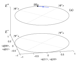
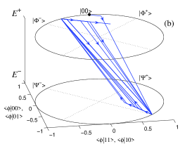
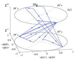
Figure 5: Examples of phase space trajectories for $r=0.5$ with initial state $|\phi^{+}(0)\rangle=|00\rangle$ and $\epsilon=1$. See text for description.

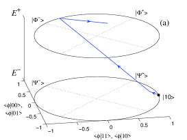
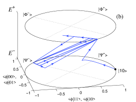
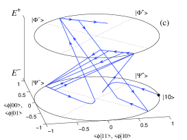
Figure 6: Examples of phase space trajectories for $r=0.5$ with initial state $|\phi^{-}(0)\rangle=|10\rangle$ and $\epsilon=1$. See text for description.

IV.3.3 Initial states $|00\rangle$ and $|10\rangle$

In Fig. 5 we plot three typical phase-space trajectories for $r=0.5$ and $|\phi^{+}(0)\rangle=|00\rangle$. Fig. 5(a) illustrates the case where the system evolves directly to the steady state $|\phi_{1}\rangle$. The probability of this event is $\left|\langle 00|\phi_{1}\rangle\right|^{2}=1/(1+r^{2})=0.8$, so it is the most likely occurrence for the chosen parameters. If a first quantum jump does occur, then typical trajectories are shown in Figs. 5(b) and (c). Following the jump to $|\phi\rangle=-|\Psi^{-}\rangle$ in $E^{-}$, a second jump returning the state to $E^{+}$ is guaranteed. For $r=0.5$, this leaves the system in the state $|\phi\rangle=0.89|00\rangle-0.45|11\rangle$, from which the probability of a further cycle of jumps is $4r^{2}/(1+r^{2})^{2}=0.64$. Thus, after a first quantum jump cycle, it is most likely that further cycles will follow, as seen in Figs. 5(b) and (c), where in both cases a total of five cycles (ten photon detections) occur before the system finally reaches the steady state.

In Fig. 6 we plot three typical phase-space trajectories for $r=0.5$ and $|\phi^{-}(0)\rangle=|10\rangle$. In this case, at least one quantum jump is certain to occur, following which the probability of further jumps is $4r^{2}/(1+r^{2})^{2}=0.64$, as above. So for this initial condition, the most likely outcome is a sequence of quantum jump cycles following a first guaranteed photon detection. In Fig. 6 (a) only the first detection occurs, while in Figs. 6(b) and (c) this detection is followed by a sequence of cycles before the steady state is eventually achieved.

IV.4 Quantum Trajectories for $r=1$

The case $r=1$ is of particular interest. The normalized eigenstates of the evolution between quantum jumps are the Bell states $|\phi_{1}\rangle=|\Phi^{+}\rangle$, $|\phi_{2}\rangle=|\Phi^{-}\rangle$, $|\phi_{3}\rangle=|\Psi^{+}\rangle$, and $|\phi_{4}\rangle=|\Psi^{-}\rangle$. The eigenvalues are $\lambda_{1}=\lambda_{3}=0$ and $\lambda_{2}=\lambda_{4}=-4$. The action of the jump operator $\hat{C}_{1}$ on states within $E^{+}$ simplifies to

$$\mkern-45.0mu\hat{C}_{1}\left(\begin{array}[]{c}c_{11}\\ 0\\ 0\\ c_{00}\end{array}\right)\rightarrow\textrm{sign}\{c_{11}-c_{00}\}|\Psi^{-}\rangle,$$ (44a)

and its action on states within $$E^{-}$$ to

$$\hat{C}_{1}\left(\begin{array}[]{c}0\\ c_{10}\\ c_{01}\\ 0\end{array}\right)\rightarrow\textrm{sign}\{c_{10}-c_{01}\}|\Phi^{-}\rangle.$$ (44b)

For $$r=1$$, photon detections, if they occur, are associated with collapses onto one of two maximally-entangled Bell states.

For initial states $|\phi^{+}(0)\rangle$ and $|\phi^{-}(0)\rangle$ in $E^{+}$ and $E^{-}$, respectively, the system evolves continuously, without the emission of any photons, to $|\phi_{1}\rangle=|\Phi^{+}\rangle$ and $|\phi_{3}\rangle=|\Psi^{+}\rangle$, with probabilities $\left|\langle\phi^{+}(0)|\Phi^{+}\rangle\right|^{2}$ and $\left|\langle\phi^{-}(0)|\Psi^{+}\rangle\right|^{2}$. Alternatively, a photon is detected with associated quantum jump to $|\Psi^{-}\rangle$ in $E^{-}$ or $|\Phi^{-}\rangle$ in $E^{+}$. In this case, as both terminal states are unstable under the between-jump evolution, a second detection and quantum jump must follow. According to Eqs. (44a) and (44b) this simply exchanges $|\Psi^{-}\rangle$ for $|\Phi^{-}\rangle$ and vice-versa. Hence, a perpetual switching between Bell states $|\Psi^{-}\rangle$ and $|\Phi^{-}\rangle$ occurs. We designate this behavior an entangled-state cycle.

Thus, at resonance we find a distinctly bimodal behavior. The system either evolves into a maximally-entangled Bell state without emitting photons, or an entangled-state cycle is initiated under which the system switches indefinitely between orthogonal Bell states while emitting a continual stream of photons. As an aside, such behavior can be regarded as a quantum measurement that distinguishes the Bell states $|\Phi^{\pm}\rangle$ from $|\Psi^{\pm}\rangle$.

The two alternative outcomes of the quantum trajectory evolution are illustrated in Figs. 7 and 8 for the initial states $|\phi^{+}(0)\rangle=|00\rangle$ in $E^{+}$ and $|\phi^{-}(0)\rangle=|10\rangle$ in $E^{-}$, respectively. With this choice of initial states there are equal probabilities for reaching the steady states, $|\Phi^{+}\rangle$ [Fig. 7(a)] and $|\Psi^{+}\rangle$ [Fig. 8(a)], and for commencing an entangled-state cycle [Figs. 7(b) and 8(b)]. Note that once an entangled-state cycle is initiated, the trajectory remains in a plane orthogonal to the lines defining $|\Phi^{+}\rangle$ and $|\Psi^{+}\rangle$; the cycle continues indefinitely

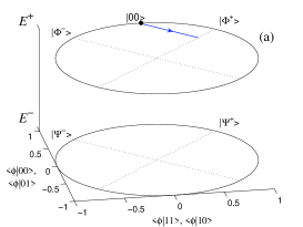
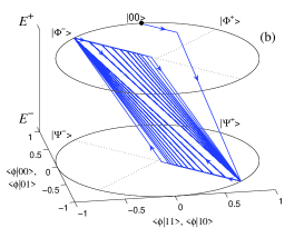
Figure 7: Examples of phase space trajectories for $r=1$ with initial state $|\phi^{+}(0)\rangle=|00\rangle$ and $\epsilon=1$. See text for description.

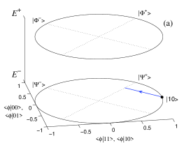
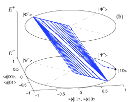
Figure 8: Examples of phase space trajectories for $r=1$ with initial state $|\phi^{-}(0)\rangle=|10\rangle$ and $\epsilon=1$. See text for description.

IV.5 Imperfect Intercavity Coupling

Our original model allowed for the possibility of imperfect intercavity coupling, through the parameter $\epsilon$ and the jump operator $\hat{C}_{2}$ which describe the effects of photon loss in propagation between the two cavities. Focusing on the resonant case ($r=1$), we now consider the situation in which $\epsilon<1$. Typical trajectories for $\epsilon=0.5$ are shown in Figs. 9(a) and 10(a), with the two photon count records shown in frames (b) and (c) of the figures. Remarkably, entangled-state cycles persist, but now the system settles into one or other of two distinct cycles, involving either the symmetric or antisymmetric Bell states.

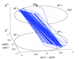
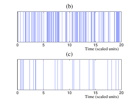
Figure 9: (a) Example of a phase space trajectory for $r=1$ with initial state $|\phi^{+}(0)\rangle=|00\rangle$ and $\epsilon=0.5$; the system eventually settles into the $|\Phi^{-}\rangle\leftrightarrow|\Psi^{-}\rangle$ entangled-state cycle. (b) and (c) Photon counts for Detectors 1 and 2, respectively.

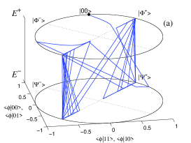
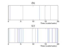
Figure 10: (a) Example of a phase space trajectory for $r=1$ with initial state $|\phi^{+}(0)\rangle=|00\rangle$ and $\epsilon=0.5$; the system eventually settles into the $|\Phi^{+}\rangle\leftrightarrow|\Psi^{+}\rangle$ entangled-state cycle. (b) and (c) Photon counts for Detector 1 and 2, respectively.

To understand the behavior, consider the forms of the operators involved; in particular, for $r=1$, we have effective Hamiltonian

$$-i\hat{H}_{\rm eff}=\left(\begin{array}[]{cccc}-2&0&0&2\sqrt{\epsilon}\\ 0&-2&2\sqrt{\epsilon}&0\\ 0&2\sqrt{\epsilon}&-2&0\\ 2\sqrt{\epsilon}&0&0&-2\\ \end{array}\right),$$ (45)

and jump operators

$$\hat{C}_{1}=\sqrt{2}\left(\begin{array}[]{cccc}0&-1&\sqrt{\epsilon}&0\\ -1&0&0&\sqrt{\epsilon}\\ \sqrt{\epsilon}&0&0&-1\\ 0&\sqrt{\epsilon}&-1&0\\ \end{array}\right),$$ (46a)

and

$$\hat{C}_{2}=\sqrt{2(1-\epsilon)}\left(\begin{array}[]{cccc}0&0&1&0\\ 0&0&0&1\\ 1&0&0&0\\ 0&1&0&0\\ \end{array}\right).$$ (46b)

Significantly, these operators commute with one another,

$$[\hat{C}_{1},\hat{C}_{2}]=[\hat{C}_{1},\hat{H}_{\rm eff}]=[\hat{C}_{2},\hat{H}_{\rm eff}]=0.$$ (47)

Their operation upon the Bell states is given by

$$-i\hat{H}_{\rm eff}|\Phi^{\pm}\rangle = -2\left(1\mp\sqrt{\epsilon}\right)|\Phi^{\pm}\rangle=\lambda_{\pm}|\Phi^{\pm}\rangle,\mkern 30.0mu$$ (48a)

$$-i\hat{H}_{\rm eff}|\Psi^{\pm}\rangle = -2\left(1\mp\sqrt{\epsilon}\right)|\Psi^{\pm}\rangle=\lambda_{\pm}|\Psi^{\pm}\rangle,$$ (48b)

and

$$\hat{C}_{1}|\Phi^{\pm}\rangle = (\lambda_{\pm}/\sqrt{2}\,)|\Psi^{\pm}\rangle,$$ (49a)

$$\hat{C}_{1}|\Psi^{\pm}\rangle = (\lambda_{\pm}/\sqrt{2}\,)|\Phi^{\pm}\rangle,$$ (49b)

$$\hat{C}_{2}|\Phi^{\pm}\rangle = \pm\sqrt{2(1-\epsilon)}|\Psi^{\pm}\rangle,$$ (49c)

$$\hat{C}_{2}|\Psi^{\pm}\rangle = \pm\sqrt{2(1-\epsilon)}|\Phi^{\pm}\rangle.$$ (49d)

Thus, the Bell states are eigenstates of $\hat{H}_{\rm eff}$, and the jump operators interchange Bell states in $E^{+}$ and $E^{-}$: each jump operator converts the symmetric (antisymmetric) Bell state in $E^{+}$ to the symmetric (antisymmetric) Bell state in $E^{-}$ and vice-versa.

Now, let us consider a particular quantum trajectory for which a total of $n$ jumps occur, separated by the time intervals $\{\Delta t_{i}:i=1,\ldots,n\}$. For an initial state $|\phi_{0}\rangle$, the (unnormalized) state at the conclusion of the $n$ jumps is written as

$$|\phi_{t}\rangle=\hat{J}_{n}e^{-i\hat{H}_{\rm eff}\Delta t_{n}}\ldots\hat{J}_{2}e^{-i\hat{H}_{\rm eff}\Delta t_{2}}\hat{J}_{1}e^{-i\hat{H}_{\rm eff}\Delta t_{1}}|\phi_{0}\rangle,$$

where each $\hat{J}_{i}$ is either $\hat{C}_{1}$ or $\hat{C}_{2}$. Since all operators in the string acting on $|\psi_{0}\rangle$ commute, this expression can be rewritten in a variety of forms, two of which prove to be especially useful in explaining the distinct behaviors illustrated by Figs. 9 and 10. In the first case, we may write

$$|\phi_{t}\rangle_{\rm(i)}=\hat{C}_{2}^{m}e^{-i\hat{H}_{\rm eff}t}\left(\hat{C}_{1}^{l}|\phi_{0}\rangle\right),$$ (50a)

passing all $$l \hat{C}_{1} m \hat{C}_{2} l+m=n$$ ocurrences of to the right and all occurrences of to the left (); in the second we write

$$|\phi_{t}\rangle_{\rm(ii)}=\hat{C}_{1}^{l}\hat{C}_{2}^{m}\left(e^{-i\hat{H}_{\rm eff}t}|\phi_{0}\rangle\right),$$ (50b)

where all jump operators are passed to the left.

The arbitrary (pure) initial state can be expressed as a superposition of Bell states,

$$|\phi_{0}\rangle=a|\Phi^{+}\rangle+b|\Phi^{-}\rangle+c|\Psi^{+}\rangle+d|\Psi^{-}\rangle,$$ (51)

where $a$, $b$, $c$, and $d$ are expansion coefficients, generally complex. Substituting this expansion into Eqs. (50a) and (50b), and using Eqs. (48a)–(49d)—assuming for simplicity that $l$ and $m$ are even—the two forms for the state $|\phi_{t}\rangle$ are

$$|\phi_{t}\rangle_{\rm(i)} \propto e^{-i\hat{H}_{\rm eff}t}|\phi_{0}\rangle^{\prime},$$ (52a)

$$|\phi_{t}\rangle_{\rm(ii)} \propto \hat{C}_{1}^{l}|\phi_{t}\rangle^{\prime},$$ (52b)

where

$$|\phi_{0}\rangle^{\prime} \equiv \lambda_{+}^{l}(a|\Phi^{+}\rangle+c|\Psi^{+}\rangle)+\lambda_{-}^{l}(b|\Phi^{-}\rangle+d|\Psi^{-}\rangle),$$

$$|\phi_{t}\rangle^{\prime} \equiv e^{\lambda_{+}t}(a|\Phi^{+}\rangle+c|\Psi^{+}\rangle)+e^{\lambda_{-}t}(b|\Phi^{-}\rangle+d|\Psi^{-}\rangle).$$

Observe now that the ratio of the eigenvalues satisfies

$$\lambda_{+}/\lambda_{-}=(1-\sqrt{\epsilon})/(1+\sqrt{\epsilon})<1.$$ (54)

It follows that $|\phi_{t}\rangle_{\rm(i)}$ and $|\phi_{t}\rangle_{\rm(ii)}$ allow us to predict quite distinct asymptotic behaviors for the system state. For sufficiently large $l$, the contribution to $|\phi_{t}\rangle_{\rm(i)}$ from the symmetric Bell states is negligible compared with the contribution from the antisymmetric Bell states, in which case, using Eqs. (52a) and (LABEL:eq:cycle1prime),

$$|\phi_{t}\rangle_{\rm(i)}\sim e^{\lambda_{-}t}\lambda_{-}^{l}\left(b|\Phi^{-}\rangle+d|\Psi^{-}\rangle\right).$$ (55)

The system is locked into a cycle between the two antisymmetric Bell states, the situation illustrated in Fig. 9 (for $\epsilon=0.5$, $\left|\lambda_{+}/\lambda_{-}\right|=0.17$). In contrast, for sufficiently large $t$, the contribution to $|\phi_{t}\rangle_{\rm(ii)}$ from the antisymmetric Bell states is negligible compared with that from the symmetric Bell states, and using Eqs. (52b) and (LABEL:eq:cycle2prime),

$$|\phi_{t}\rangle_{\rm(ii)}\sim e^{\lambda_{+}t}\left(\frac{\lambda_{+}}{\sqrt{2}}\right)^{l}\left(b|\Phi^{+}\rangle+d|\Psi^{+}\rangle\right).$$ (56)

The system is locked into a cycle between the two symmetric Bell states, as shown in Fig. 10.

Which of the two cycles is chosen in a particular realization of the photon counting record is random, as is the time taken to settle into the cycle. Effectively, the decision is the outcome of a competition between the periods of evolution between quantum jumps and the jumps themselves—specifically, those associated with photon counts at Detector 1. Considering Eqs. (LABEL:eq:cycle1prime) and (54), we see that every count at Detector 1 results in an increased probability to find the system in one of the antisymmetric Bell states. On the other hand, from Eqs. (LABEL:eq:cycle2prime) and (54), the periods of evolution between counts have the reverse effect—they increase the probability for the system to be found in a symmetric Bell state. The critical factor that decides which tendency wins is the number of photon counts occuring at Detector 1 over a given (substantial) interval of time. If there are many, as in Fig. 9(b), the entangled-state cycle between antisymmetric Bell states wins out; if there are few, Fig. 10(b), the cycle between symmetric Bell states occurs. The same decision mechanism is observed in other examples Carmichael94 . Note that counts at Detector 2 are not involved—not directly at least. They do figure indirectly as a mechanism reducing the average number of counts at Detector 1; indeed, they are the ultimate source of the asymmetry reflected in the ratio $\lambda_{+}/\lambda_{-}<1$.

As the system approaches a particular cycle the quantum trajectory evolution tends to reinforce the establishment of the cycle. Close to the antisymmetric cycle, the evolution between jumps is dominantly governed by $\lambda_{-}=-2(1+\sqrt{\epsilon})$ and is therefore relatively fast. This leads to frequent photon counts at Detector 1 [Fig. 9(b)]. Close to the symmetric cycle, the between-jump evolution is dominantly governed by $\lambda_{+}=-2(1-\sqrt{\epsilon})$, hence is relatively slow. Photon counts at Detector 1 become much less frequent [Fig. 10(b)].

From the dramatic difference in count rates at Detector 1 for the two cycles, it is clear that one can determine which entanglement cycle the system evolves to for a particular realization. However, without knowledge of the record of photon counts at Detector 2, which by definition we do not have, one can not know where on the cycle the system is, i.e., whether the state is in $E^{+}$ or $E^{-}$. Thus, the ensemble average state of the system is mixed, described by one of the density operators

$$\rho_{\pm}=\frac{1}{\sqrt{2}}\left(|\Phi^{\pm}\rangle\langle\Phi^{\pm}|+|\Psi^{\pm}\rangle\langle\Psi^{\pm}|\right).$$ (57)

V Discussion and Conclusions

Consider a thought experiment where the cascaded qubit system, set to resonance, evolves freely and its entire output is collected and stored inside a black box. At some time the lasers driving the Raman transitions are turned off, so the evolution ceases. The box and qubits are separated and moved to causally disconnected regions of space time. Let Alice and Bob be standard observers of the qubits, and give Eve jurisdiction over the box.

We can now ask, how much entanglement exists between the qubits of Alice and Bob? While this is simply a roundabout way of asking how entanglement evolves, it helps elucidate some of the key concepts behind the quantum trajectory measure of entanglement. Conventional entanglement measures are based upon an analysis of the density matrix at this time. They throw away the box and look at the system of qubits alone—they disregard Eve and view the system from the perspective of Alice and Bob.

Yet in general every interaction between two objects entangles them, and as the qubit system and box interacted in the past, their states are intertwined. Neither possess an independent reality, and neither, considered alone, can be completely described. Eve’s box contains information, which, if discarded, adds entropy to the qubit system of Alice and Bob. This entropy is the source of ambiguity in the quantification of entanglement. From this point of view, as noted in the introduction, the problem of bi-partite entanglement in an open system relates to that of tri-partite entanglement in a closed one. To completely characterize the entanglement of the present example, in addition to the entanglement between Alice and Bob, we must consider their entanglement with Eve.

A quantum description of the box is impractical, but it is feasible to extract classical information about what it contains, through measurement. Quantum trajectories facilitate this, and allow us not to discard the box completely. In turn, the system state retains its purity, conditional on the classical information extracted from the box. With this extra information, we can extract more entanglement from the cascaded qubit system.

Working from the master equation for the cascaded system Clark03 , previously it was assumed that the system evolved gradually into a pure state, whereby entanglement was generated. The behaviour at resonance, however, was unclear, since there the master equation had two zero eigenvalues and no well-defined steady state. By considering the conditional evolution we have shown that, at resonance, asymptotically the system is either in the Bell state $|\Phi^{+}\rangle$ or oscillating (stochastically switching) between two Bell states, $|\Phi^{-}\rangle$ and $|\Psi^{-}\rangle$.

From the density matrix point of view, the latter is an equal mixture of Bell States and would yield no entanglement under any mixed state measure; physically, Alice and Bob, without collaboration from Eve, cannot extract any entanglement from their qubits. Suppose, however, that Eve opens her box to count the number of photons inside. Seeing whether the count is even or odd, she is able to deduce exactly which Bell state Alice and Bob’s system is in. Thus, her measurement unravels the density operator, creating entanglement, despite the fact that the measurement is not causally connected to Alice and Bob’s qubits.

It is tempting to say that the entanglement was always there, as a matter of fact, until one realizes that there are many other ways in which Eve could choose to measure her state, each producing a different unravelling of the qubit system and yielding a different value of entanglement. The entanglement facilitated by Eve’s measurements is contextual in this sense.

This thought experiment demonstrates why any attempt to quantify the entanglement of an open system from the density operator alone cannot be considered complete. The density operator should not be treated as a fundamental object, as it does not provide a complete description of the physical state. We have presented a simple example where oscillations between maximally entangled states are hidden within a separable density operator. The fact that the density operator contains entropy, implies that information about its entanglement with an external system was discarded at some time. In studying such a mixed state, there is benefit from considering, not only the mixed state itself, but the process through which it was generated, and the access this potentially gives to a conditional dynamics.

The results of this paper could be extended by employing quantum trajectories in a broader sense. In cases where the results of environmental interactions cannot be measured, such as coupling loss, Wiseman and Vaccaro wiseman1 have shown that only certain unravelings can be physically realized. A conceivable measure of entanglement would take the minimum of all physically realizable unravelings. Alternatively, one might take the maximum of all physically realizable unravellings, which would measure the maximum distillable entanglement when local measurements on the environment are taken into account.

This work was supported by the Marsden Fund of the RSNZ.

References

- (1) M. A. Nielsen and I. L. Chuang, Quantum Computation and Quantum Information (Cambridge University Press, Cambridge, 2000).
- (2) C. H. Bennett, D. P. DiVincenzo, J. A. Smolin, and W. K. Wootters, Phys. Rev. A 54, 3824 (1996).
- (3) C. H. Bennett, H. J. Bernstein, S. Popescu, and B. Schumacher, Phys. Rev. A 53, 2046 (1996).
- (4) M. Horodecki, P. Horodecki, and R. Horodecki, Phys. Rev. Lett. 84, 2014 (2000).
- (5) H. Nha and H. J. Carmichael, Phys. Rev. Lett. 93, 120408 (2004).
- (6) H. J. Carmichael, An Open Systems Approach to Quantum Optics, Lecture Notes in Physics Vol. 18 (Springer-Verlag, Berlin, 1993).
- (7) A. R. R. Carvalho, M. Buse, O. Brodier, C. Vivienscas, and A. Buchleitner, quant-ph/0510006.
- (8) S. Clark, A. Peng, M. Gu, and S. Parkins, Phys. Rev. Lett. 91, 177901 (2003).
- (9) S. M. Tan, Quantum Optics and Computation Toolbox for Matlab, available at http://www.qo.auckland.ac.nz.
- (10) H. M. Wiseman and J. A. Vaccaro, Phys. Rev. Lett. 87, 240402 (2001).
- (11) H. J. Carmichael, P. Kochan, and L. Tian, “Coherent states and open quantum systems: a comment on the Stern-Gerlach experiment and Schrödinger cats,” in Coherent States: Past, Present, and Future, eds. D. H. Feng, J. R. Klauder, and M. R. Strayer (World Scientific, Singapore, 1994), pp. 75-91.