High order non-unitary split-step decomposition of unitary operators

Abstract

We propose a high order numerical decomposition of exponentials of hermitean operators in terms of a product of exponentials of simple terms, following an idea which has been pioneered by M. Suzuki, however implementing it for complex coefficients. We outline a convenient fourth order formula which can be written compactly for arbitrary number of noncommuting terms in the Hamiltonian and which is superiour to the optimal formula with real coefficients, both in complexity and accuracy. We show asymptotic stability of our method for sufficiently small time step and demonstrate its efficiency and accuracy in different numerical models.

1 Introduction

While exponentials of operators are very common in every field of quantum physics, but also in classical physics, their evaluation is nevertheless numerically a very demanding operation. For example, in quantum physics, this task usually emerges when one wants to compute a time-evolution, either in real time, for example when computing dynamical correlations, or in imaginary time, when computing thermodynamic averages like in quantum Monte Carlo simulations. A similar decomposition of classical time evolution, which can also be interpreted in terms of unitary operators, is known as symplectic integration.

For an operator which can be written as a sum of several parts of which exponential operators are exactly determinable, the well known Suzuki-Trotter[1, 2, 3, 4, 5, 6, 7] decomposition scheme can be used. The operator $e^{\mathrm{i}z\sum_{j}A_{j}}$ is approximated by a product of operators $e^{\mathrm{i}zp_{k_{j}}A_{j}}$ with real coefficients $p_{k}$ such that the desired order of accuracy is achieved. We will show in the present paper that following the same principles but not restricting to real coefficients the same order can be achieved using a smaller number of factors. Furthermore, the order of such decomposition can be trivially increased by one by composing it with an equivalent decomposition with a complex conjugate set of coefficients. We will outline a particular third order scheme, and further improved to fourth order, which is potentially very useful for practical calculations. We show explicitly that, even though we lose unitarity of decomposition (in real-time case), the method is asymptotically stable for sufficiently small time steps since all the eigenvalues of the decomposition remain on the complex unit circle. Even more generally, we show that one gains an extra order in accuracy and asymptotic stability (independent of the size of the time step) by renormalizing the state vector after each time step.

We demostrate the accuracy and efficiency of the method by three explicit examples: (i) in case of $2\times 2$ matrices the decomposition and its stability can be treated analytically, (ii) for exponentials of Gaussian random Hermitean matrices we find that the stability threshold (the maximal time-step for which the method is asymptotically stable) drops with the inverse power of the dimension of the matrix, and (iii) for a generic (non-integrable) interacting spin $1/2$ chain (in one-dimension) we find, surprisingly, that the stability threshold is independent of the number of spins.

2 Complex Split-Step Decomposition

Our main objective is to approximate the exponential operator $U_{0}=e^{\mathrm{i}z(A+B)}$, for general bounded operators $A$ and $B$, and a complex parameter $z$, as a product $U$ of exponential operators

$$\mathrm{e}^{\mathrm{i}z(A+B)}=\mathrm{e}^{\mathrm{i}zp_{1}A}\mathrm{e}^{\mathrm{i}zp_{2}B}\mathrm{e}^{\mathrm{i}zp_{3}A}\mathrm{e}^{\mathrm{i}zp_{4}B}\mathrm{e}^{\mathrm{i}zp_{5}A}+\mathcal{O}(z^{4}).$$ (1)

The equations determining the coefficients $\{p_{j}\}$ that solve the equation above are obtained by expanding the exponential operators into power series and equating lowest order terms to zero. It is known that there is no third order ($\mathcal{O}(z^{4})$) solution of the five-term ansatz (1) with real coeffients $p_{j}$. The simplest third order decomposition involves six terms [5]. However, allowing the coefficients $p_{j}$ to be complex, there exist two very simple and symmetric solutions, namely

$$p_{1}=\overline{p_{5}}=\frac{1}{4}+\frac{\sqrt{3}}{12}\mathrm{i},\quad p_{2}=\overline{p_{4}}=\frac{1}{2}+\frac{\sqrt{3}}{6}\mathrm{i},\quad p_{3}=\frac{1}{2}$$ (2)

and the complex conjugate set $\{\overline{p_{j}}\}$.

Let us denote exact exponential as $U_{0}(z)=\exp(\mathrm{i}z(A+B))$ and third order complex decompositions (C3), given by RHS of (1) with coefficients (2), namely $\{p_{j}\}$, and $\{\overline{p_{j}}\}$, as $U(z)$ and ${\overline{U}}(z)$, respectively. Using some further analysis (which has been performed by means of Mathematica software) we can show that the next-order-term changes sign when one switches between the two solutions, namely:

$$U(z)=U_{0}(z)+K_{4}z^{4}+\mathcal{O}(z^{5})\quad\textrm{and}\quad{\overline{U}}(z)=U_{0}(z)-K_{4}z^{4}+\mathcal{O}(z^{5}),$$ (3)

where

$$K_{4} = \frac{\mathrm{i}}{144\sqrt{3}}((AAAB-BAAA)-3(AABA-ABAA)-$$ (4)

$$\quad\enskip-3(AABB-BBAA)+6(ABAB-BABA)+$$

$$\quad\enskip+2(ABBB-BBBA)+6(BABB-BBAB))$$

is a Hermitean operator provided that both $A$ and $B$ are Hermitean.

Superposition of the two decompositions cancels the $z^{4}$ term and is therefore for one order higher, namely of fourth order. However, the same, fourth, order can be achieved by alternating both decompositions (as illustrated in fig. 1)

$${\overline{U}}(z)U(z)=U_{0}^{2}+(U_{0}K_{4}-K_{4}U_{0})z^{4}+\mathcal{O}(z^{5})=U_{0}^{2}+\mathcal{O}(z^{5}),$$ (5)

since $U_{0}(z)=1+\mathcal{O}(z)$. Since in usual numerical simulations of exponential operators, for example in quantum time-evolutions, time dependent renormalization group methods, or quantum Monte-Carlo simulations, one needs to make many time-steps anyway, the alternation between $U(z)$ and ${\overline{U}}(z)$ does not represent any practical drawback.

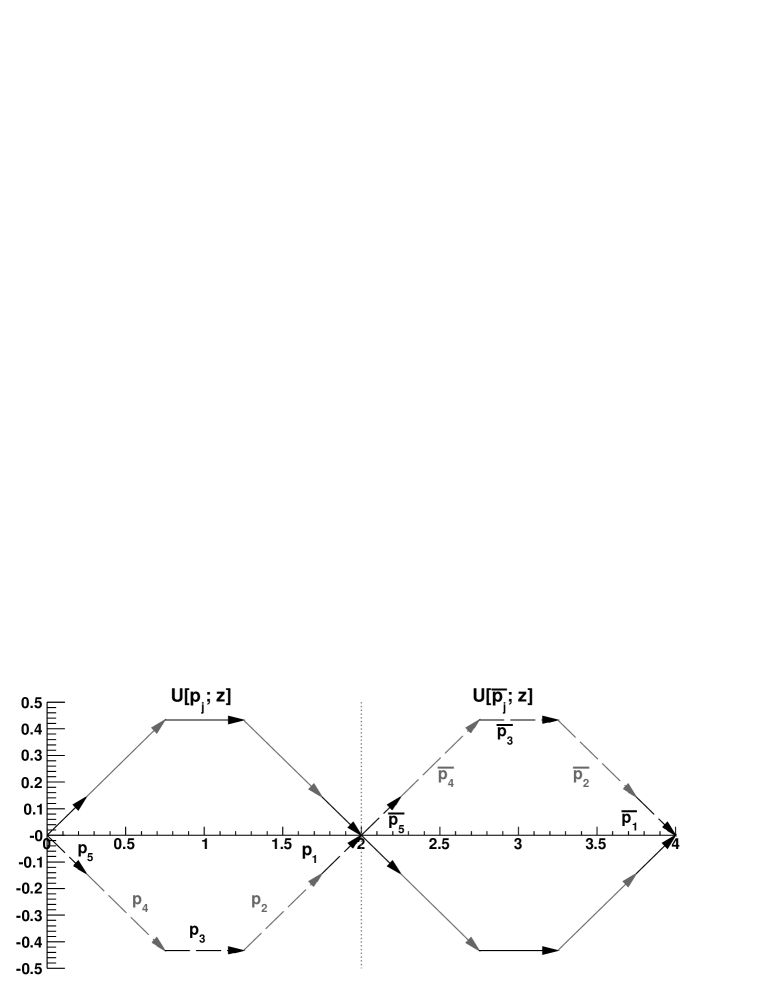
Figure 1: Schematic illustration of complex valued split step decomposition. Coefficients $p_{j}$ can be considered as shifts in complex time plane, which always move along the real axis. Two sets of complex coefficients $\{p_{i}\}$ give a third order decomposition $\mathcal{O}(z^{4})$; their superposition is for an order higher.

However, we note that with $p_{i}$ being complex numbers the decomposition $U(z)$ is no longer strictly unitary (in the usual case where the operators $A$ and $B$ are Hermitean and the time step $z$ is real) and the time evolved state (on which $U$ operates) might explode in norm after a while. In order to strictly preserve the norm, the state (vector) may be renormalized at every time step. One might be afraid that this renormalization would degrade the accuracy of the method. However, due to the fact $K_{4}^{\dagger}=K_{4}$ this is not the case, in fact renormalization increases the accuracy to fourth order

$$\frac{\langle U_{0}^{\dagger}(z)U(z)\rangle}{\sqrt{\langle U^{\dagger}(z)U(z)\rangle}}=\frac{1+\langle K_{4}\rangle z^{4}+\mathcal{O}(z^{5})}{\sqrt{1+\langle K_{4}+K_{4}^{\dagger}\rangle z^{4}+\mathcal{O}(z^{5})}}=1+\mathcal{O}(z^{5}).$$ (6)

By $\langle.\rangle:=\langle\psi|.|\psi\rangle$ we denote the expectation value in some intial state vector $|\psi\rangle$. In conclusion, the decomposition with one single set of complex coefficients $p_{i}$ (C3) is already of the fourth order (${\mathcal{O}}(z^{5})$) if every time step is followed by renormalization of the state (fig. 2). As in any application the computational complexity of performing the sequence of exponential operators on a state vector $U(z)|\psi\rangle$ is dominating the normalization of the state, this does not represent any drawback of the method. Still, as we will show later, the method is asymptotically stable, for sufficiently small $z$ even without the renormalization. Figure 2 shows real numerical errors, in a model in which $A$ and $B$ are chosen as Gaussian random Hermitean matrices, after performing two time steps with various decompositions described above (using one (C3) or both sets of complex coefficients (C4), and with or without renormalization of the state) and compare it with the optimal third order decomposition with real coefficients (R3).

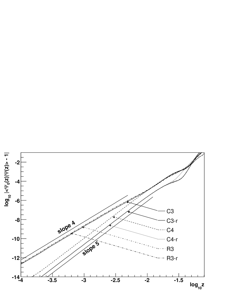
Figure 2: An error after two time steps for the third-order real decomposition (R3), the third-order complex decomposition (C3), and the fourth-order complex decomposition (C4); the label ’r’ denotes renormalization after each time step. As for numerical model we choose $A$ and $B$ to be GUE matrices of dimension $N=200$ and average the results over 1000 realizations.

We can easily generalize our approach to approximate exponentials of three or more noncommuting bound operators. For example, for three operators, one has nine terms following a sequence $ABCBABCBA$ which is obtained from $ABABA$ (1) by replacing each inner operator $B$ by $BCB$ (and dividing the coefficient in front of $B$ by two)

$$\mathrm{e}^{\mathrm{i}z(A+B+C)}=\mathrm{e}^{\mathrm{i}zp_{1}A}\mathrm{e}^{\mathrm{i}zp_{1}B}\mathrm{e}^{\mathrm{i}zp_{2}C}\mathrm{e}^{\mathrm{i}zp_{1}B}\mathrm{e}^{\mathrm{i}zp_{3}A}\mathrm{e}^{\mathrm{i}zp_{4}B}\mathrm{e}^{\mathrm{i}zp_{5}C}\mathrm{e}^{\mathrm{i}zp_{4}B}\mathrm{e}^{\mathrm{i}zp_{5}A}+\mathcal{O}(z^{4})$$ (7)

and using the same set of coefficients (2), or its complex conjugate. Generally, a formula for a sum of $n$ operators involves $4n-3$ terms

$$\exp\left(\mathrm{i}z(A_{1}+\ldots A_{n})\right)=$$

$$\mathrm{e}^{\mathrm{i}zp_{1}A_{1}}\mathrm{e}^{\mathrm{i}zp_{1}A_{2}}\cdots\mathrm{e}^{\mathrm{i}zp_{1}A_{n-1}}\mathrm{e}^{\mathrm{i}zp_{2}A_{n}}\mathrm{e}^{\mathrm{i}zp_{1}A_{n-1}}\cdots\mathrm{e}^{\mathrm{i}zp_{1}A_{2}}\times$$

$$\mathrm{e}^{\mathrm{i}zp_{3}A_{1}}\mathrm{e}^{\mathrm{i}zp_{5}A_{2}}\cdots\mathrm{e}^{\mathrm{i}zp_{5}A_{n-1}}\mathrm{e}^{\mathrm{i}zp_{4}A_{n}}\mathrm{e}^{\mathrm{i}zp_{5}A_{n-1}}\cdots\mathrm{e}^{\mathrm{i}zp_{5}A_{2}}\mathrm{e}^{\mathrm{i}zp_{5}A_{1}}.$$ (8)

It is interesting to note that the general optimal third order solution with real coefficients (R3) uses just one term more for the case $n=2$, namely six, whereas for general $n$ case it needs $5n-4$ terms, which is $n-1$ terms more than the complex solution above (8).

As we have mentioned before, without the renormalization complexness of the coefficients may cause the exponential instability of the method. However, it turns out that the decomposition is absolutely stable for small enough steps $z$. The reason for such an interesting behaviour is that the eigenvalues of the operator $U(z)$ lie all on complex unit circle for sufficiently small $z$, and this property grants the asymptotic stability even if $U(z)$ is not exactly unitary. There is typically a threshold, i.e. a critical value of $z_{\rm max}$ such that at $z=z_{\rm max}$ two eigenvalues of $U(z)$ collide and leave the unit circle and then the method ceases to be asymptotically stable. Such a behaviour can be explicitly proven for operators chosen from the space of $2\times 2$ matrices (see the following section) and is conjectured in general.

3 Examples

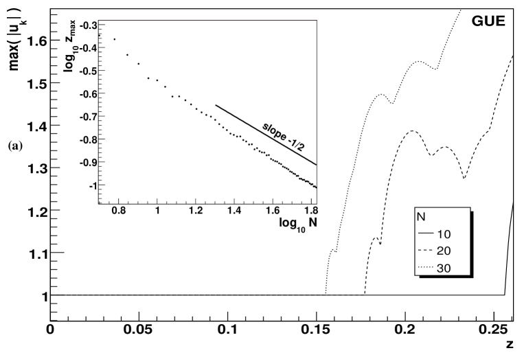
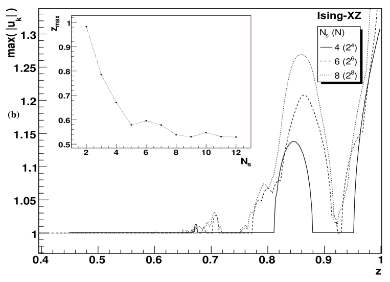
Figure 3: Maximal size of the eigenvalue of the approximate evolution operator $U(z)$. The upper plot (a) shows the case of GUE matrices while the lower plot (b) shows the case of Ising spin chain in tilted magnetic field (see text). Different curves refer to systems of different sizes (b), or different matrix dimensions (a). The insets show critical threshold $z_{\rm max}$ as a function of the system size/matrix dimension.

First, let us consider a numerical example of calculating the exponential of $H=A+B$ where $A$ and $B$ are Gaussian random Hermitean matrices chosen at random from the Gaussian Unitary Ensemble [9]. Figure 3a shows that the maximal size of eigenvalue of $U(z)$ is exactly equal to one until some point described by the threshold step size $z_{\rm max}$. Numerical results suggest the following dependence of the threshold on the Hilbert space dimension $N$, $z_{\rm max}\propto 1/N^{\alpha}$, with $\alpha\approx 0.5$, which we believe is the worst case scenario for generic systems.

As a second example, we consider a non-trivial physical model where the matrices of operators $A$ and $B$ are very sparse and thus far from the full random matrix model, namely we consider time evolution in the quantum Ising spin 1/2 chain in a tilted homogeneous magnetic field (e.g. recently considered in the context of heat transport [10]) described by the hamiltonian $H=\sum_{n=1}^{N}\left\{-J\sigma_{n}^{z}\sigma_{n+1}^{z}+g_{x}\sigma_{n}^{x}+g_{z}\sigma_{n}^{z}\right\}$. Here, $\sigma_{n}^{x,y,z}$, $n=1\ldots N_{s}$, represent a set of independent Pauli matrices. In figure 3b we show a very interesting result for this model (in particular, for the parameter values $J=1$, $g_{x}=0.4$, $g_{z}=0.8$ which lie in the so-called “quantum chaotic” regime [10]), namely that the threshold step size $z_{\rm max}$ is asymptotically independent of the size $N=2^{N_{s}}$ of the system. We conjecture that this is in general true for numerical simulations of finite (spin) quantum systems with local interaction, and for such our method of simulation of time-evolution should be very roboust.

As for the last example, we make analytical consideration of the simplest case where our operators can be represented by $2\times 2$ matrices. In order to understand the transition in the stability (collision of eigenvalues of $U(z)$ on the unit circle) one can generally parametrize the operators $A$ and $B$ by Pauli operators $\sigma^{j}$, $j=1,2,3$,

$$A=a_{0}1+\sum_{j=1}^{3}a_{j}\sigma^{j}\quad\textrm{and}\quad B=b_{0}1+\sum_{j=1}^{3}b_{j}\sigma^{j}.$$ (9)

The coefficients $\{a_{j}\}$, and $\{b_{j}\}$ are all real since matrices $A$ and $B$ are Hermitean, and furthermore matrices $A$ and $B$ can always be chosen traceless by setting $a_{0}=b_{0}=0$ without losing generality. It is obvious that, since $\det U=e^{\mathrm{i}z\textrm{Tr}H}$, where $H=A+B$, that decomposition (1) for two $2\times 2$ matrices can also be expressed in terms of Pauli matrices and some coefficients $\{g_{j}\}$. Using the ansatz (1) we write

$$\mathrm{e}^{\mathrm{i}zp_{1}\sum_{j}a_{j}\sigma^{i}}\mathrm{e}^{\mathrm{i}zp_{2}\sum_{j}b_{j}\sigma^{i}}\mathrm{e}^{\mathrm{i}zp_{3}\sum_{j}a_{j}\sigma^{i}}\mathrm{e}^{\mathrm{i}zp_{4}\sum_{j}b_{j}\sigma^{i}}\mathrm{e}^{\mathrm{i}zp_{5}\sum_{j}a_{j}\sigma^{i}}=\mathrm{e}^{\mathrm{i}z\sum_{j}g_{j}\sigma^{j}}.$$ (10)

Of course, $g_{j}$ are no longer real in general. Eigenvalues of the operator $U(z)=e^{\mathrm{i}z\sum_{j}g_{j}\sigma^{j}}$ are $e^{\pm\mathrm{i}z\sqrt{\sum_{j}g_{j}^{2}}}$ which gives the condition for the asymptotic stability: namely the number $\gamma^{2}=\sum_{j}g_{j}^{2}$ should be real and positive, $\gamma^{2}\in\mathbf{R}^{+}$. In order to simplify the notation, let us take $\gamma=+\sqrt{\sum_{j}g_{j}^{2}}$, and similarly write $\alpha=\sqrt{\sum_{j}a_{j}^{2}},\beta=\sqrt{\sum_{j}b_{j}^{2}}$, and introduce normalized coefficients $\gamma_{i}=g_{i}/\gamma,\alpha_{j}=a_{j}/\alpha,\beta_{j}=b_{j}/\beta$. The condition for asymptotic stability now simply reads $\gamma\in\mathbf{R}$. Using straightforward calculation $\gamma$ can be expressed as $\gamma=\frac{1}{z}\arccos(\frac{1}{2}\textrm{Tr}\,e^{\mathrm{i}z\sum_{i}g_{i}\sigma_{i}})$ and is, interestingly, only a function of the magnitudes $\alpha$, $\beta$ and z-projections $\alpha_{3}$ and $\beta_{3}$:

$$\gamma(z) = \frac{1}{z}\arccos Q(z),\quad\textrm{where}$$

$$Q(z) = \frac{1}{8}\Bigg{(}\Big{(}1-\alpha_{3}^{2}+(1+3\alpha_{3}^{2})\cos(\alpha z)\Big{)}\Big{(}(1+\beta_{3}^{2})\cos(\beta z)+$$ (11)

$$+ (1-\beta_{3}^{2})\cosh(\frac{\beta z}{\sqrt{3}})\Big{)}-2\alpha_{3}(3+\alpha_{3}^{2})\beta_{3}\sin(\alpha z)\sin(\beta z)+$$

$$+ 2(1-\alpha_{3}^{2})\cosh(\frac{\alpha z}{2\sqrt{3}})\Big{(}(1+\beta_{3}^{2})\cos(\frac{\alpha z}{2})\cos(\beta z)+$$

$$+ (1-\beta_{3}^{2})\cos(\frac{\alpha z}{2})\cosh(\frac{\beta z}{\sqrt{3}})-2\alpha_{3}\beta_{3}\sin(\frac{\alpha z}{2})\sin(\beta z)\Big{)}\Bigg{)}$$

Now the stability condition reduces to $\left|Q(z)\right|\leq 1$. For small steps $z$ the expression $Q(z)$ in (11) can be written as a power series in $z$

$$Q(z)=1-\frac{1}{6}(\alpha^{2}+\beta^{2}+2a_{3}^{2}+2b_{3}^{2}+6a_{3}b_{3})z^{2}+\mathcal{O}(z^{4}).$$ (12)

It can easily be proven diagonalizing the quadratic form that the $z^{2}$ term is always nonpositive, hence the decomposition scheme indeed is always (for any $a_{j},b_{j}$) stable, for small steps $z$.

Figure 4: Illustration of the stability threshold for $2\times 2$ case. Since matrices are traceless, collision of eigenvalues of $U(z)$ takes place on the real axis. In the figure we plot ${\rm Re}\gamma$ (dashed) and ${\rm Im}\gamma$ (full), as a function of $z$ for the case $\alpha=\beta=1$ and $\alpha_{3}=\beta_{3}=0.1$.

Figure 4 illustrates how eigenvalues for small steps $z$ always lie on the unit circle in the complex plane. When the step $z$ is being increased, the eigenvalues are travelling along the unit circle, one in clockwise and the other in the counter-clockwise direction. At some point, namely at $z=z_{\rm max}$, a collision occurs and a pair of eigenvalues bounce off the unit circle - then $\gamma$ becomes complex. However, because of the restriction $\left|\det U\right|=1$ their product remains on the unit circle. Our $2\times 2$ matrices $A$ and $B$ are assumed to be traceless therefore collisions always occur on the real axis and eigenvalues are both real during the bounce.

4 Conclusion

We have proposed a simplex explicit complex-coefficient split-step decomposition of an operator exponential, based on Suzuki’s scheme, for a sum of arbitrary number of operators. As compared to an optimal scheme with real coefficients our scheme requires less terms for the same order, furthermore we can gain an extra order at no additional expense. Despite having complex coefficients the decomposition is always stable for sufficiently small step size, and can be stablilized by additional renormalization of the state vector.

We suggest that our method may be used in conjunction with other methods for efficient time evolution of complex quantum systems (one application has already been done in Ref.[10]), or interacting many body quantum systems, like for example with time-dependent DMRG methods [11, 12] where efficient and accurate estimation of operator exponentials for short time steps is one of the cruicial black-box operations.

References

References

- [1] H. F. Trotter, Proc. Am. Math. Phys. 10 (1959), 545.
- [2] M. Suzuki, Commun. Math. Phys. 51 (1976), 183.
- [3] M. Suzuki, J. Math. Phys. 26 (1985), 601.
- [4] M. Suzuki, Phys. Lett. A 165 (1992), 387.
- [5] M. Suzuki, J. Phys. Soc. Japan 61 (1992), 3015.
- [6] M. Suzuki, Phys. Lett. A 146 (1990), 319.
- [7] M. Suzuki, J. Math. Phys. 32 (1991), 400.
- [8] A. D. Bandrauk and H. Shen, Chem. Phys. Lett. 176 (1991), 428.
- [9] M. L. Mehta, Random Matrices (Academic Press, London, 1991), 2nd ed.
- [10] C. Mejia-Monasterio, T. Prosen, and G. Casati, cond-mat/0504181.
- [11] S. R. White and A. E. Feiguin, Phys. Rev. Lett. 93 (2004), 076401.
- [12] G. Vidal, Phys. Rev. Lett. 93 (2004), 040502.