Degradation of a quantum reference frame

Abstract

We investigate the degradation of reference frames, treated as dynamical quantum systems, and quantify their longevity as a resource for performing tasks in quantum information processing. We adopt an operational measure of a reference frame’s longevity, namely, the number of measurements that can be made against it with a certain error tolerance. We investigate two distinct types of reference frame: a reference direction, realized by a spin-$j$ system, and a phase reference, realized by an oscillator mode with bounded energy. For both cases, we show that our measure of longevity increases quadratically with the size of the reference system and is therefore non-additive. For instance, the number of measurements that a directional reference frame consisting of $N$ parallel spins can be put to use scales as $N^{2}$. Our results quantify the extent to which microscopic or mesoscopic reference frames may be used for repeated, high-precision measurements, without needing to be reset – a question that is important for some implementations of quantum computing. We illustrate our results using the proposed single-spin measurement scheme of magnetic resonance force microscopy.

I Introduction

In quantum measurement theory, the apparatus is generally treated as a classical system – one that is not described by the quantum formalism. The same is true for the macroscopic systems that serve as reference frames, for instance, a ruler with respect to which positions are defined, a set of gyroscopes with respect to which orientations are defined, or a clock with respect to which phases are defined. Just as attempts to quantize the measurement apparatus have led many researchers to foundational puzzles (such as the quantum measurement problem), the quantization of reference frames has also generated its fair share of confusion and controversy (Ref. BRS05 provides a synopsis and numerous references).

In addition to providing, through such puzzles, an opportunity for us to refine our understanding of quantum theory, the quantization of reference frames is also useful for answering certain practical questions. In many quantum experiments, one can understand certain systems as constituting mesoscopic or even microscopic reference frames to which other systems are compared. In such cases, the conventional approach wherein reference frames suffer no back-action may yield a poor approximation to a full quantum treatment.

A recent example is the investigation of how well a quantum optical field prepared in a coherent state can serve as a local oscillator for homodyne detection Tyc04 . It has also been proposed that the finite size of a reference frame can lead to effective decoherence on the system it describes in contexts ranging from collapse theories Fin05 to the evaporation of black holes Gam04 . In particular, there have been several investigations into the consequences of the quantum nature of laser fields for the manipulation of physical qubits in quantum information processing Enk02 ; Gea02 .

Our goal in this paper is to go beyond consideration of how the finite size of the reference frame affects the purity or coherence of systems described with respect to it, and to examine how this finiteness affects its longevity i.e., how many times it can be used in a measurement as an accurate reference frame. In particular, we demonstrate quantitatively how, if one makes measurements of the “orientation” of a large number of systems relative to a single quantum reference frame (RF), then as a result of these measurements the state of the RF becomes more mixed, more symmetric and is thereafter less useful for implementing the sorts of tasks for which an RF is required. This degradation (and ultimate depletion) is yet another reason (in addition to those provided in BRS03 ; Vac03 ; BRS04a ; Enk05 ) for considering RFs as an information-theoretic resource.

At first glance, one might expect that the longevity of an RF, quantified by the number of estimations of the relative orientation of a system to the RF that one can achieve with a certain error bound before it degrades beyond use, would scale linearly with the size of the RF. For example, if two identical directional RFs were used together, one would naively expect the resulting combined RF to last twice as long as either constituent RF would separately. However, our analysis shows that the scaling does not match this expectation. In fact, the longevity of such a directional RF scales quadratically with the number of spins $N$. We show that the same scaling holds for a phase reference, such as a coherent state. Specifically, the longevity of such a phase reference scales quadratically in the average excitation number (e.g., photon number). This result is encouraging for the potential usefulness of mesoscopic reference frames in quantum information processing applications.

We illustrate this point with a simple calculation for single-spin measurements using magnetic resonance force microscopy, demonstrating both that this measurement scheme may exhibit effects due to the degradation of its directional RF with repeated use, but also that it may be possible to use such a device for the large number of measurement required for quantum computing applications without significant degradation.

We emphasize the distinction between the quality of an RF, which describes how well a quantum RF approximates an ideal classical RF for the purposes of measurement, and the longevity of an RF, which describes how many times it can be used in a measurement whilst maintaining a certain quality. Whereas general uncertainty-principle-based arguments can often be used to determine the scaling of the quality of a quantum RF, we are unaware of any such argument that can predict the quadratic scaling of the longevity that we determine in this paper.

II Preliminaries

We define the longevity of a reference frame as the number of times it can be used to perform a particular operational task with some chosen finite degree of success. To explain the particular task we choose, it is convenient to be able to compare our RF with another, much larger “background” RF. We denote the RF whose longevity we are studying by $R$, which is initially correlated (aligned) with the background RF. (In Ref. BRS05 , a RF $R$ with this feature was referred to as implicated.) For example, $R$ may be a gyroscope used in a laboratory experiment, to which directional systems are compared, and the background RF could be the frame defined by the earth or the fixed stars.

The task to which $R$ will be put to use is the estimation of the direction of a system $S$ relative to the background RF. (We here use the term “direction” in a generic way to mean the group element relating $S$ to the background RF even if the the group of transformations in which we are interested is not the rotation group). Such an estimation is achieved by measuring the relation between $S$ and $R$, then combining the outcome with one’s prior information about the directionality of $R$ relative to the background RF, to deduce something about the direction of $S$ relative to the background RF. However, because $R$ is a finite quantum system, the measurement of the relation between $S$ and $R$ causes a disturbance to the quantum state of $R$, so that after this measurement, one’s ability to infer the directionality of another system $S^{\prime}$ is decreased. Thus, $R$ can only be used a finite number of times for such a task before its directionality relative to the background RF is so poorly defined that it is no longer useful for this purpose. It is this degradation that we investigate.

Because neither $S$ nor $R$ physically interacts with the background RF during the task of interest, we can take the background RF to be non-dynamical. (More precisely, because the dynamics induced between $R$ and $S$ is completely relational, we will see that the use of the background RF is equivalent to simply choosing a convenient gauge and has no bearing on the physics). The RF $R$, on the other hand, must be treated dynamically. Consequently, we assign a Hilbert space and quantum states to $R$ but not to the background RF. Adopting the terminology of Ref. BRS05 , $R$ is treated as an internal RF, while the background RF is treated as an external RF. We shall also say that we are treating $R$ as a quantum RF, and the background RF as a classical RF.

A few aspects of our direction-estimation task must be made specific. First, there is the nature of the measurement that determines the relation between $S$ and $R$. To be conservative, we assume: (1) the measurement is the one that maximizes one’s ability to estimate the relation between $S$ and $R$, and thus also maximizes one’s ability to estimate the direction of $S$ relative to the background RF (the figure of merit for estimation will be specified later) and (2) the measurement is implemented in a manner that leads to the smallest possible degradation of $R$ while still satisfying feature (1). Feature (2) ensures that we are determining the best possible longevity for a given degree of success in direction-estimation. Taking into account the fact that the more information we gain in the measurement, the more disturbance we create, feature (1) ensures that the longevity we derive will be a lower bound for the number of uses to which $R$ can be put for any other sort of direction estimation task on $S$.

The second aspect of our estimation task that must be made specific is the initial quantum state of $R$. We choose to investigate the state that leads to the least initial error in estimating the directionality of $S$ relative to the background RF. We emphasize that, although the optimal RF states and optimal measurements may not necessarily be easy to achieve in practice, they establish the quantum limit and therefore bound any RF longevity.

We note that an equivalent definition of longevity can be achieved without making any reference to a background RF. In this case, our description of $S$ and $R$ would be subject to an effective superselection rule for the group that is associated with the RF BDSW04 . For instance, if the RF is for orientation, then moving to a description that makes no reference to the background RF would imply adopting an effective non-Abelian superselection rule for the group of rotations SU(2). Although the usefulness of this mode of description has been emphasized elsewhere BRS05 , we shall not make use of it in the present paper. In what follows, we assign quantum states to $S$ and $R$ that are non-invariant under the group of interest, even though the measurement of the relation of $S$ to $R$ is invariant under this group. That is, the quantum states are assigned relative to an arbitrary background RF, which is not used in the measurement. One may liken this procedure to choosing a gauge for convenience when describing gauge-invariant processes.

III Directional reference frame

In this section, we study the degradation of a directional RF, that is, a reference for a direction in space. (Note that a directional RF does not provide a full Cartesian frame, as it does not provide a reference for rotations about its axis.)

III.1 Measurement of a spin-1/2 system relative to a spin-$j$ directional RF

We use a spin-$j$ system for our quantum directional RF, with Hilbert space $\mathbb{H}_{j}$. The initial quantum state of the spin-$j$ system is denoted $\rho^{(0)}$. (Later, in Sec. III.3, we will determine the state that minimizes the error in the estimation of direction.) We describe this RF relative to a background RF, as noted in Sec. II, and choose it to be aligned in the $+z$ direction relative to the background RF; we emphasise, though, that this alignment with a background RF is essentially a choice of gauge. Because the quantum RF will serve only as a reference direction, and not a full frame, we can choose it to be invariant under rotations about the $\hat{z}$ axis without loss of generality. Thus, the initial quantum state, $\rho^{(0)}$ is diagonal in the $|j,m\rangle$ basis of $\mathbb{H}_{j}$, that is, the basis of simultaneous eigenstates of $\hat{J}^{2}$ and $\hat{J}_{z}$.

The systems to be measured against the quantum RF will be spin-1/2 systems, each with a Hilbert space $\mathbb{H}_{1/2}$. We choose the initial state of each such system to be the completely mixed state $I/2$, where $I$ is the identity operator on $\mathbb{H}_{1/2}$. This corresponds to maximal ignorance about the spin-1/2 system. Our quantum RF will be used to measure many such independent spin-1/2 systems sequentially. We shall assume trivial dynamics between measurements, and thus our time index will simply be an integer specifying the number of measurements that have taken place. The state of the RF following the $n$th measurement is denoted $\rho^{(n)}$, with $\rho^{(0)}$ denoting the initial state of the RF prior to any measurement. We consider the state of the RF from the perspective of someone who has not kept a record of the outcome of previous measurements. Thus, at every measurement, we average over the possible outcomes with their respective weights to obtain the final density operator.

A measurement of the relative orientation of a spin-1/2 particle to a spin-$j$ system is represented by operators that are invariant under collective rotations. The measurement that provides the maximum information gain about the relative orientation between a spin-$j$ and a spin-$j^{\prime}$ system has been determined in BRS04b . It is simply a measurement of the magnitude of the total angular momentum $\hat{J}^{2}$. That is, it is the projective measurement $\{\Pi_{J}\}$, where $\Pi_{J}$ projects $\mathbb{H}_{j}\otimes\mathbb{H}_{j^{\prime}}$ onto the total $\hat{J}^{2}$ eigenspace with eigenvalue $J(J+1)$. For the case where $j^{\prime}=1/2$, the optimal measurement for determining the relative orientation is represented by the two-outcome projective measurement $\{\Pi_{+}\equiv\Pi_{j+1/2},\Pi_{-}\equiv\Pi_{j-1/2}\}$ on $\mathbb{H}_{j}\otimes\mathbb{H}_{1/2}$ BRS04b .

III.2 Measurement-induced update of the directional RF state

A given projective measurement can be associated with many different update maps. As discussed in Sec. II, we choose the update map that is minimally disturbing. In App. A, it is shown that this corresponds to adopting the Lüders rule for updating: for a measurement outcome associated with the projector $\Pi,$ the quantum state $\rho$ is updated to $\Pi\rho\Pi/\mathrm{Tr}(\rho\Pi).$

Thus, under the optimal measurement for relative orientation, the evolution of the quantum RF as a result of the $n$th measurement is

$$\rho^{(n+1)}=\mathcal{E}(\rho^{(n)})$$ (1)

where

$$\mathcal{E}(\rho)=\text{Tr}_{S}\Bigl{(}\sum_{c\in\{+,-\}}\Pi_{c}(\rho\otimes I/2)\Pi_{c}\Bigr{)}\,,$$ (2)

and $\text{Tr}_{S}$ denotes the partial trace over the spin-1/2 system.

The map $\mathcal{E}$ can be written using the operator-sum representation Nie00 as

$$\mathcal{E}(\rho)=\frac{1}{2}\sum_{c\in\{+,-\}}\sum_{a,b\in\{0,1\}}E_{ab}^{c}\rho E_{ab}^{c{\dagger}}\,,$$ (3)

where

$$E_{ab}^{c}\equiv\left\langle a\right|\Pi_{c}\left|b\right\rangle$$ (4)

is a Kraus operator on $\mathbb{H}_{j}$ and $\{\left|0\right\rangle,\left|1\right\rangle\}$ is a basis for $\mathbb{H}_{1/2}$. These operators can be straightforwardly determined in terms of Clebsch-Gordon coefficients.

We note that the evolution of the RF is not unitary (and would not be unitary even if the measurement result was kept), because the quantum RF becomes entangled with the measured system which is subsequently discarded. Thus, the map $\mathcal{E}$ is irreversible and consequently one may say that the quantum state of the RF undergoes decoherence.

In App. B, we provide a recurrence relation for the matrix elements of the state $\rho^{(n)}$.

III.3 Measure of directional RF quality

One simple measure of how much the RF degrades is the fidelity Nie00 between the state after $n$ measurements, $\rho^{(n)}$, and the initial state, $\rho^{(0)}$, which clearly decreases with $n$. Another natural measure is the asymmetry of the state Vac05 , which also is found to decrease with $n$. However, rather than use these measures, we will instead choose to quantify the quality of the RF operationally as the average probability of a successful estimation of the orientation of a spin-1/2 system in a pure state (relative to the background RF). For simplicity, we assume that this fictional “test” spin-1/2 system is with equal probability either aligned or anti-aligned with the background RF. It is worth making special note of the fact that in the sequence of measurements that cause the RF degradation, the state of the spin-1/2 system is not assumed to be a pure state that is aligned or anti-aligned with the RF. It is assumed to be completely mixed. However, after each measurement we ask: if a spin-1/2 system in such a pure state were compared to the RF, how well could we estimate whether it was aligned or antialigned?

Denote the pure state of the test spin-1/2 system that is aligned (anti-aligned) with the initial RF by $|0\rangle$ ($|1\rangle$). For a spin-1/2 system prepared in the state $|0\rangle$, the probability of success, that is, of finding the correct ($j+1/2$) result, is

$$P_{\mathrm{s}}^{0}(n)=\mathrm{Tr}\Bigl{(}\bigl{[}\rho^{(n)}\otimes|0\rangle\langle 0|\bigr{]}\Pi_{+}\Bigr{)}=\mathrm{Tr}_{R}(\rho^{(n)}E_{00}^{+})\,.$$ (5)

Similarly, for a spin-1/2 system prepared in the state $|1\rangle$, the probability of the correct $(j-1/2)$ result is $P_{\mathrm{s}}^{1}(n)=\mathrm{Tr}_{R}(\rho^{(n)}E_{11}^{-})$. Thus, the average probability of success is

$$\overline{P}_{\mathrm{s}}(n)=\frac{1}{2}\mathrm{Tr}_{R}(\rho^{(n)}(E_{00}^{+}+E_{11}^{-}))\,.$$ (6)

Using Clebsch-Gordon coefficients to determine the Kraus operators of Eq. (4), we find

$$\overline{P}_{\text{s}}(n)=1-\tfrac{1}{(2j+1)}\sum_{m=-j}^{j}(j-m+1/2)\textrm{Tr}_{R}(\rho^{(n)}|j,m\rangle\langle j,m|)\,.$$ (7)

We remind the reader that, at every measurement, the resulting density matrix for the RF has been averaged over the possible previous outcomes with their respective weights. Thus, this measure $\overline{P}_{\text{s}}(n)$ is applicable to situations where the prior measurement record is discarded. In addition, this method also quantifies the average case longevity even if the measurement record is kept.

We now focus our attention on a particular initial state of the RF. We choose the state that is optimal for our measure of RF quality, in other words, we choose the $\rho^{(0)}$ that maximizes $\overline{P}_{\text{s}}(0)$. This involves minimizing the sum in Eq. (7), which may be written as

$$\mathrm{Tr}(M\rho^{(0)})\,,$$ (8)

where

$$M=\sum_{m=-j}^{j}(j-m+1/2)\left|j,m\right\rangle\left\langle j,m\right|\,.$$ (9)

Clearly then, we should choose $\rho^{(0)}$ to be an eigenvector of $M$ associated with the smallest eigenvalue, namely, $\rho^{(0)}=\left|j,m=j\right\rangle\left\langle j,m=j\right|.$ Thus we see that the quantum state that maximizes our measure of quality of the RF is an SU(2) coherent state, yielding $\overline{P}_{\mathrm{s}}(0)=1-1/[2(2j+1)]$.

(This result is not in conflict with that of Peres and Scudo Per01 , where it was demonstrated that the product state of $N$ parallel spins (which is equivalent to the SU(2) coherent state) was not the optimal state for the transmission of a reference direction, because their system was not assumed to be a spin-$j$ representation, as we have done here. An interesting direction for future work is to extend the results of Lin05 in order to determine the optimal measurements of spin-1/2 systems against these more general RF systems and to explore the degradation in this case.)

III.4 Scaling of the longevity of a directional RF with size

Our problem is to solve Eq. (1) to determine the RF state as a function of $n$. In the limit $j\gg 1,$ one can obtain a closed-form expression for the diagonal elements of the state of the RF at step $n$, assuming an initial state $\rho^{(0)}=|j,j\rangle\langle j,j|$. It is

$$\textrm{Tr}(\rho^{(n)}|j,m\rangle\langle j,m|)\\ =(-1)^{j-m}\binom{n}{j-m}(j-m)!(-2j)U(j-m+1,n+2,-2j)\,,$$ (10)

where $U(a,b,z)$ is Kummer’s $U$ function AS . Details are given in App. B.

Using this result, we find the rate at which $\overline{P}_{\text{s}}(n)$ decreases with $n$ to be

$$\overline{P}_{\text{s}}(n)=\tfrac{1}{2}+\tfrac{j}{2j+1}(1-\tfrac{2}{(2j+1)^{2}})^{n}\,.$$ (11)

We plot this for various values of $j$ in Fig. 1.

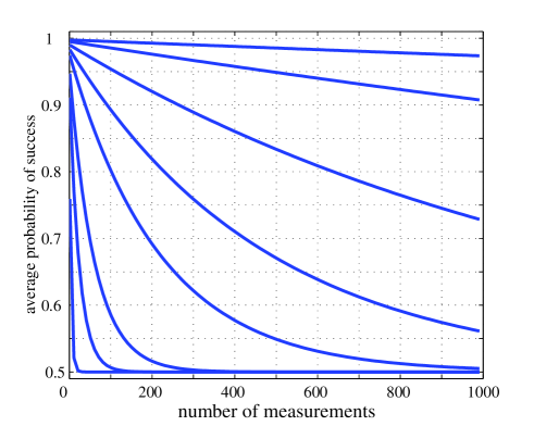
Figure 1: A plot of the success probability for a test particle to be measured correctly against the directional reference frame, versus the number of previous spins that have been measured against the frame. The plots (from bottom left to top right) are for a reference frame of spin $j=1,3,5,10,15,25,50,100$, respectively.

The initial slope of this function bounds the rate of degradation. It is

$$R\equiv\overline{P}_{\text{s}}(1)-\overline{P}_{\text{s}}(0)=-2j/(2j+1)^{3}\,.$$ (12)

Thus, in the large $j$ limit, we have the rate of degradation with $n$ satisfying $R\geq-1/(4j^{2})$.

Let $\epsilon<1$ be a fixed allowed error probability for the spin-1/2 direction estimation problem. After $n$ measurements, the probability of successful estimation is lower bounded by $1+nR$, so the number of measurements required to ensure that this bound be greater than $1-\epsilon$ is $-\epsilon/R$. Consequently, the number of measurements that can be implemented relative to the spin-$j$ RF with probability of error less than $\epsilon$ is

$$n_{\mathrm{max}}\simeq\epsilon j^{2}\,.$$ (13)

This result implies that the number of measurements for which an RF is useful, that is, the longevity of a RF, increases quadratically rather than linearly with the size of the RF.

Numerical calculation of the longevity’s dependence on RF size for various choices of error threshold confirm this result; see Fig. 2.

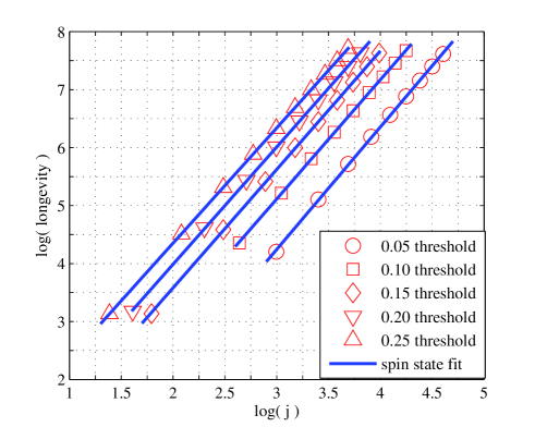
Figure 2: A loglog plot of the longevity (number of measurements before the error probability for a test particle exceeds a fixed threshold) of a directional reference frame versus the size of the frame. Plots for various different error thresholds are given. A clear quadratic asymptotic dependence emerges despite the relatively small reference frames indicated: linear regression yields gradients which all lie within $2\pm 0.1$.

This result implies that, in order to maximize the number of measurements that can be achieved with a given error thereshold, one should combine all of one’s directional RF resources into a single large RF and perform all measurements relative to it. It is also worth noting that if the directional RF is composed out of $N$ spin-1/2 systems, so that it has size $j=N/2+1,$ the number of measurements that can be performed with probability of error less than $\epsilon$ scales as $N^{2},$ whereas one might have naïvely thought that it would be good for only as many measurements as there are constituent spins. Finally, note that an SU(2) coherent state for $N$ spin-1/2 systems is a product state so that entanglement does not appear to be responsible for this property.

III.5 Application to single-spin measurement using magnetic resonance force microscopy for solid-state quantum computing

The physical nature of measurement apparatuses and reference systems is particularly relevant for quantum computation. The stringent requirements placed on measurement devices for use in quantum computing include (i) large coupling strengths, often requiring the measurement device to be made very small and placed close to the quantum registers (qubits); and (ii) the apparatuses must be well-described by classical, noiseless devices in order to obtain the required levels of accuracy (e.g., perform projective von Neumann measurements). These two requirements appear at first glance to be mutually exclusive, but may be satisfied by novel mesoscopic measurement schemes. Consider, as an example, the proposal to use magnetic resonance force microscopy (MRFM) to measure the direction of a single spin Sid95 ; Rug04 in a solid-state quantum computer. This scheme makes use of a small magnet placed on the tip of a nano-mechanical resonator; monitoring the oscillations of the resonator can be used to measure the direction of a spin placed near the magnet. To couple strongly to a single spin, the measurement device must be cold and very small (i.e., a resonator with a mass of the order of picograms, with a magnet on the tip of length scale 10 nm Sid95 ). However, objects on this scale are poorly approximated as classical, macroscopic measurements apparatuses, and thus a semi-classical or full quantum treatment of the measuring device is required.

The results we have presented here can be applied to the proposed use of MRFM to measure the direction of a single spin, and its associated applications to solid-state quantum computing. The design parameters of a scheme to obtain single-spin measurement are outlined in Sid95 , in which the magnet consists of an iron sphere of diameter $\sim 300$ Å. Treated as a quantum system, then, the magnet can be approximately described by $10^{6}$ parallel spins. With an error tolerance of $10^{-4}$ (a reasonable threshold for quantum computation) this RF would perform $10^{8}$ optimal measurements before degrading beyond further usefulness. Thus, if the measurement scheme can be chosen such that the disturbance on the RF due to each measurement is comparable with that of the optimal update map, it appears that a mesoscale RF such as this may be suitable for repeated use in large-scale quantum computation.

IV Phase reference

We now consider the case of a phase reference. Our systems will consist of oscillator modes, taken to be optical modes for clarity. It should be noted that we focus on the optical case only to make the description of the results less abstract; the results are applicable to any phase reference.

IV.1 Measurement of single-rail qubit relative to phase reference

For our phase reference, we take a single oscillator mode with Hilbert space denoted by $\mathbb{H}_{R}$. (Note that we could instead use a multimode phase reference, or even many qubits prepared as “refbits” Enk05 .) Again, the initial quantum state of the RF is denoted $\rho^{(0)}$. We describe this RF relative to a background phase reference, and arbitrarily choose its phase to be zero (our choice of gauge).

The systems to be measured against the RF will be single-rail qubits, i.e., oscillators with states restricted to the lowest-energy 2-dimensional subspace spanned by Fock states $|0\rangle$ and $|1\rangle$. The Hilbert space is denoted $\mathbb{H}_{S}$.

We consider the particular estimation task wherein the system is promised to encode phase $0$ or phase $\pi$ with equal probability, which is to say that it is promised to be in a state $\left|+\right\rangle$ or $\left|-\right\rangle$, where $\left|\pm\right\rangle=2^{-1/2}\left(\left|0\right\rangle\pm\left|1\right\rangle\right)$, with equal probability. In this case, an optimal measurement for estimating whether the relative phase between system and quantum RF is $0$ or $\pi$ is the two-outcome projective measurement $\{\Pi_{+},\Pi_{-}\}$ with

$$\Pi_{+} =\sum_{m=1}^{\infty}|m,{+}\rangle\langle m,{+}|+|0\rangle_{R}\left\langle 0\right|\otimes\left|0\right\rangle_{S}\langle 0|$$

$$\Pi_{-} =\sum_{m=1}^{\infty}|m,{-}\rangle\langle m,{-}|\,,$$ (14)

where

$$|m,\pm\rangle=\frac{1}{\sqrt{2}}\bigl{(}|m\rangle_{R}|0\rangle_{S}\pm|m{-}1\rangle_{R}|1\rangle_{S}\bigl{)}\,.$$ (15)

This is demonstrated in App. C.

It is worth noting that this measurement is a coarse-graining of the optimal projective measurement of phase Bag05 on each of the 2-dimensional eigenspaces of total photon number; we further note that this measurement was used in Ver03 for the same purpose.

We will be interested in determining how the RF state evolves after many such measurements on distinct systems. For simplicity, we consider the RF state as it is described by an observer who does not know whether the system was in the state $\left|+\right\rangle$ or $\left|-\right\rangle$ initially, and because the two are presumed equally likely, the initial state of the system is presumed to be the completely mixed state $I$/2. We also assume that the observer does not keep track of the results of the measurements.

IV.2 Measurement-induced update of the phase reference

As with the directional example, the update rule for this two-outcome projective measurement that is minimally-disturbing is the Lüders rule, described in App. A.

With this choice of update rule, the evolution of the quantum RF as a result of the $n$th measurement has the same form as Eqs. (1-4) but where the $E_{ab}^{c}$ operators are now given by

$$E_{00}^{+}=\tfrac{1}{2}(I_{R}+|0\rangle\langle 0|)\,,\quad E_{00}^{-}=\tfrac{1}{2}(I_{R}-|0\rangle\langle 0|)\,,$$ (16)

$$E_{11}^{+}=E_{11}^{-}=\tfrac{1}{2}I_{R}\,,$$ (17)

$$E_{10}^{+}=-E_{10}^{-}=(E_{01}^{+})^{{\dagger}}=-(E_{01}^{-})^{{\dagger}}=\tfrac{1}{2}A\,,$$ (18)

where $I_{R}$ is the identity on $\mathbb{H}_{R}$ and

$$A\equiv\sum_{m=0}^{\infty}|m\rangle\langle m+1|\,.$$ (19)

The update map due to a single measurement is therefore

$$\mathcal{E}(\rho)=\tfrac{1}{2}\rho+\tfrac{1}{4}|0\rangle\langle 0|\rho|0\rangle\langle 0|+\tfrac{1}{4}A^{{\dagger}}\rho A+\tfrac{1}{4}A\rho A^{{\dagger}}\,.$$ (20)

Again we note that although it may be difficult to achieve such an update map in practice, it is nonetheless interesting to consider because it defines the quantum limit of RF longevity. If the systems under consideration are modes of the electromagnetic field, this update map is particularly impractical given current technology because it corresponds to a quantum non-demolition measurement on the electromagnetic field. An interesting problem for future research is to determine how much degradation, in excess of the quantum limit, is incurred by the use of more realistic update maps.

IV.3 Measure of phase reference quality

As with the directional case, we operationally quantify the quality of the RF at step $n$ as the average probability of success in a hypothetical measurement of whether a qubit system is in phase or out of phase with the background phase reference, that is, whether the qubit is in the state $\left|+\right\rangle$ or $\left|-\right\rangle,$ given equal prior probability for these two possibilities. Denoting the state of the RF at step $n$ by $\rho^{(n)}$, and using the optimal measurement (14), the average success rate is found to be

$$\overline{P}_{\mathrm{s}}(n)=\frac{1}{2}+\frac{1}{2}\sum_{m=0}^{\infty}\text{Re}\Bigl{(}\rho_{m,m+1}^{(n)}\Bigr{)}\,.$$ (21)

where $\rho_{m,m+1}^{(n)}\equiv\textrm{Tr}(\rho^{(n)}|m\rangle\langle m+1|)$.

Just as we did for the directional case, we consider the degradation in the case of an initial state of the RF that is initially optimal for our measure of RF quality, i.e., the state $\rho^{(0)}$ that maximizes $\overline{P}_{\text{s}}(0)$. However, if the accessible Hilbert space $\mathbb{H}_{R}$ is taken to be infinite-dimensional, then this probability can trivially be made arbitrarily close to one. To obtain a non-trivial and physical result, we must bound the energy of the state $\rho^{(0)}$ in some way; we may then use this bound as a measure of the “size” of the RF, analogous to the use of total spin $j$ for the directional case.

One natural choice for implementing this bound is to limit the maximum photon number to some fixed value $N$, i.e., demand that $\rho^{(0)}$ has support entirely on the $(N+1)$-dimensional subspace spanned by $\{|m\rangle\,,\ m=0,\ldots,N\}$. We now seek the state $\rho^{(0)}$ that maximizes $\overline{P}_{\text{s}}(0)$ subject to this constraint. This requires us to maximize the expression

$$\mathrm{Tr}(M_{N}\rho^{(0)})\,,$$ (22)

where

$$M_{N}=\sum_{m=0}^{N}(|m\rangle\langle m+1|+|m+1\rangle\langle m|)\,.$$ (23)

Thus we must choose $\rho^{(0)}$ to be the eigenvector of $M_{N}$ with minimal eigenvalue. The solution is

$$\left|\psi_{N}\right\rangle=\mathcal{N}\sum_{m=0}^{N}\sin\Bigl{[}\frac{(m+1)\pi}{N+2}\Bigr{]}\left|m\right\rangle\,,$$ (24)

where $\mathcal{N}$ is a normalization factor. This is the same state that is optimal for determining the relative path length between two arms in an interferometer, for several different figures of merit Sum90 . We provide a derivation of Eq. (24) in App. D. For this state, we have

$$\overline{P}_{\mathrm{s}}(0) =\frac{1}{2}\bigl{(}1+\cos(\pi/(N+2))\bigr{)}$$

$$\simeq 1-\frac{\pi^{2}}{2N^{2}}\,,\ \text{for large}\ N\,.$$ (25)

We note, however, that our method of bounding the energy of the initial state $\rho^{(0)}$ excludes states, such as the coherent state $|\alpha\rangle=e^{-|\alpha|^{2}/2}\sum_{n=0}^{\infty}(\alpha^{n}/\sqrt{n!})|n\rangle$, that have non-zero support on the entire Hilbert space $\mathbb{H}_{R}$ but nevertheless have a finite energy. It is beyond the scope of this paper to explore all the varied possibilities for determining optimal phase references for alternate choices of bounds. However, because of the ubiquity of coherent states as phase references in many physical systems, we will also consider how the longevity of a coherent state compares with the optimal phase-encoding state with bounded number (24). We compare the size of such states through average photon number $\bar{n}$, which is given by $|\alpha|^{2}$ for a coherent state and by $N/2$ for an optimal phase-encoding state containing at most $N$ photons.

IV.4 Degradation of phase reference

To determine the rate at which $\overline{P}_{\text{s}}(n)$ decreases with $n$, given an initial state $\rho^{(0)}$ for the RF, we need only determine the evolution of the matrix elements $\rho_{m,m+1}$. To this end, we use Eq. (20) to obtain the following recurrence relation for these elements,

$$\rho_{m,m+1}^{(n+1)}=\frac{1}{2}\rho_{m,m+1}^{(n)}+\frac{1}{4}\rho_{m+1,m+2}^{(n)}+\frac{1}{4}\rho_{m-1,m}^{(n)}\,.$$ (26)

As it turns out, the elements on the $m,m+1$ diagonal depend only on elements on this diagonal at the previous time step. The solution to this recurrence relation is found to be

$$\rho_{m,m+1}^{(n)}=\frac{1}{4^{n}}\sum_{j=1}^{n+m+1}\Bigl{[}\tbinom{2n}{n-j+m}-\tbinom{2n}{n-j-m}\Bigr{]}\rho_{j,j+1}^{(0)}\,.$$ (27)

This expression can be used in Eq. (21) to determine numerically how $\overline{P}_{\text{s}}(n)$ decreases with $n$ for a given choice of initial state $\rho^{(0)}$. In Fig. 3, we plot $\overline{P}_{\text{s}}(n)$ for an initial optimal phase-encoding state with number bound $N$, Eq. (24), for various values of $N$. For comparison, we also plot $\overline{P}_{\text{s}}(n)$ for an initial coherent state with mean number $|\alpha|^{2}=N/2$ (so that we are comparing states with the same mean number of photons). We note that, although the optimal phase-encoding state with bounded number gives a superior initial probability of success $\overline{P}_{\text{s}}(0)$ when compared to that of the coherent state, the latter appears more robust and does not degrade as quickly. This result demonstrates, perhaps surprisingly, that optimizing the initial quality of a quantum reference frame (quantified by the initial probability of success) does not optimize the longevity of the state. It is an interesting line of future research to determine which quantum states give the optimal longevity.

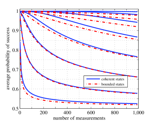
Figure 3: A plot of the success probability for a test mode to be measured correctly against the phase reference frame, versus the number of previous oscillators that have been measured against the frame. Plots are shown for both coherent states and the optimal phase-encoding states for bounded number. The plots (from bottom left to top right) are for a reference frame of average photon number $\bar{m}=1,4,9,16,25,36,49,64$, respectively. The fact that the plots for the coherent state and the optimal phase-encoding state are nearly overlapping at $\bar{m}=4$ and $9$ is a result of the similarity of the number distributions of the two states at these values of $\bar{m}$.

We find numerically that the longevity of a phase reference, both for the optimal phase-encoding state with bounded number and for the coherent state, scales as $\bar{n}^{2}$, the mean photon number squared; see Fig. 4. Specifically, we find that $\overline{P}_{\text{s}}(n)$ reaches a fixed value independent of $\bar{n}$ after a number of uses equal to $\bar{n}^{2}$. Again, we find that the number of measurements for which a phase RF is useful, that is, the longevity of a RF, increases quadratically rather than linearly with the size of the RF.

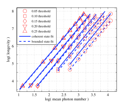
Figure 4: A loglog plot of the longevity (number of measurements before the error probability for a test particle exceeds a fixed threshold) of a phase reference frame versus the size of the frame. Plots for various different error thresholds are given. A clear quadratic asymptotic dependence emerges despite the relatively small reference frames indicated: linear regression yields slope fits which all lie within $2\pm 0.1$.

V Discussion

We have presented results on the degradation of both a directional and a phase reference. In each case we have essentially uncovered a quadratic scaling of the number of uses the frame can endure in terms of the size of the frame. An open question is whether this quadratic scaling of longevity holds for all types of RFs.

It is interesting to consider whether a semi-classical model would suffice for describing the degradation of an RF. In particular, one could employ a description of a dynamical classical RF that uses a probability distribution on the space of “orientations” which encodes one s ignorance of the exact direction, and also use a measurement theory that relates the probability of successful measurement to the uncertainty (variance) of this distribution. This uncertainty would increase with repeated measurements; a simple model might be to use diffusion (i.e., a classical random walk) to characterise this increase. Our key result in this paper is to determine the rate of degradation and its dependence on the size of the RF. If this rate was to be determined solely from a semi-classical model, then the model would require a sophisticated measurement theory for determining the direction of a quantum spin relative to a classical object of a given size. We believe that a heuristic, semi-classical model that predicts the quadratic scaling of the number of uses of an RF in terms of its size would be very desirable.

It is worth noting that we have considered only the consequences of measurements on an RF, and not the consequences of a continual interaction with an environment. In practice, RFs do interact with their environments, and so the impact on their longevity is an important question for future research. It should be noted that although many environments are likely to act in a manner similar to measurements, thereby increasing the rate of degradation, others might in fact act to continuously realign one’s quantum RF with another, larger, RF which exists in the background. For instance, if the RF is composed of a number of spins, and is continuously interacting with a strong uniform magnetic field, then thermalization will tend to cause the spins to become aligned with the field.

Spatial/directional RFs are ubiquitous, and so one might question the need for considering their degradation. It could be argued, for example, that any directional RF which has degraded can be realigned with some background RF in the lab (treated as a macroscopic directional RF) at any time. However, such realignment may prove to be difficult for microscopic apparatuses that are placed close to the quantum systems to be measured. In addition, realignment of a degraded shared RF costs resources - an issue that can be important especially within the context of quantum communication. Our main result shows, however, that such realignment may not be necessary for many situations, such as the MRFM example discussed above.

Although some RFs, such as directional RFs, are indeed ubiquitous, RFs for many other degrees of freedom are not. Some RFs must be painstakingly prepared via some controlled quantum process. One example is the BCS ground state of a superconductor, which serves as a phase reference for experiments involving superconducting qubits; another example is a Bose-Einstein condensate. An analysis similar to the one presented in this paper for any such frame could be used to determine the RF size necessary to keep errors below a specified threshold for a specified number of uses.

Although in this paper we have considered the amount of degradation that results from measurements that maximize the information gain about the relative orientation of system and RF, it is clear that there is a trade-off between longevity and information gain; the more informative the measurement, the more degradation to the RF. An interesting problem for future research is to determine the precise nature of this tradeoff.

Appendix A Proof that Lüders rule updating is minimally-disturbing

A measure of the quality of a RF, henceforth a measure of “frameness”, is operational if it quantifies the maximum success with which one can achieve some task in a variation over all protocols that use only the resource and invariant operations. Any operational measure of frameness $F$ is by definition a monotone with respect to operations that are invariant under the action of the group associated with that RF, that is, if $\rho$ is the quantum state of a RF for the group $G$, then

$$F(\mathcal{E}(\rho))\leq F(\rho)\,,$$ (28)

for all $\mathcal{E}$ that are invariant under $G,$ that is, for which $\mathcal{E}\left[U(g)(\cdot)U^{{\dagger}}(g)\right]=U(g)\mathcal{E}(\cdot)U^{{\dagger}}(g)$ for all $g\in G$. We call such measures frameness monotones.

The maximum probability of a successful estimation of a direction of a system relative to a quantum reference frame is clearly an operational measure of frameness (it involves a variation over all estimation protocols that use invariant operations and the RF resource). It is therefore by definition a frameness monotone.

We now make use of the following proposition concerning CP maps that are update maps for a projective measurement.

Proposition: For any map $\mathcal{E}$ such that $\mathcal{E}^{{\dagger}}(I)=\Pi,$ where $\Pi$ is a projector, we have

$$\mathcal{E}(\rho)=\mathcal{E}(\Pi\rho\Pi)\,.$$ (29)

Proof. Any Krauss decomposition of $\mathcal{E}$ is of the form

$$\mathcal{E}(\rho)=\sum_{\mu}K_{\mu}\rho K_{\mu}^{{\dagger}}\,,$$ (30)

with

$$\sum_{\mu}K_{\mu}^{{\dagger}}K_{\mu}=\Pi\,.$$ (31)

Given that every term in the sum is positive, that is, $K_{\mu}^{{\dagger}}K_{\mu}\geq 0$, it follows that

$$\text{supp}(K_{\mu}^{{\dagger}}K_{\mu})\subseteq\text{supp}(\Pi)\,,$$ (32)

where supp$(A)$ denotes the support on the Hilbert space of the operator $A$.  It follows that

$$\text{supp}(\sqrt{K_{\mu}^{{\dagger}}K_{\mu}})\subseteq\text{supp}(\Pi)\,,$$ (33)

and thus

$$\sqrt{K_{\mu}^{{\dagger}}K_{\mu}}=\sqrt{K_{\mu}^{{\dagger}}K_{\mu}}\Pi\,.$$ (34)

But now using the polar decomposition $K_{\mu}=U_{\mu}\sqrt{K_{\mu}^{{\dagger}}K_{\mu}}$, we infer that

$$K_{\mu}=K_{\mu}\Pi\,.$$ (35)

Our claim then follows trivially. QED.

Now, by virtue of the fact that $\mathcal{E}$ is invariant under $G$, and by virtue of the fact that the probability of successful estimation of a direction, $P_{\text{s}},$ is a frameness monotone, it follows that

$$P_{\text{s}}(\mathcal{E}(\rho)) =P_{\text{s}}(\mathcal{E}(\Pi\rho\Pi))$$ (36)

$$\leq P_{\text{s}}(\Pi\rho\Pi)$$ (37)

Normalizing our density operators, we have

$$P_{\text{s}}(\frac{\mathcal{E}(\rho)}{\text{Tr}\left(\Pi\rho\right)})\leq P_{\text{s}}(\frac{\Pi\rho\Pi}{\text{Tr}\left(\Pi\rho\right)})\,.$$ (38)

Thus the probability of successful estimation given a Lüders rule collapse map $\rho\rightarrow\Pi\rho\Pi/\mathrm{Tr}(\Pi\rho)$ is an upper bound for the probability of successful estimation for any collapse map associated with $\Pi.$   Thus one can do no better than to use the Lüders rule collapse map.

Appendix B Derivation of the recurrence relation for a directional RF

In order to explicitly solve for the degraded state $\rho^{(n)}$ of a directional RF as a function of $n$, we now derive a recurrence relation for the matrix elements of the state. The $E_{ab}^{c}$ operators can be obtained in the $|j,m\rangle$ basis using Clebsch-Gordon coefficients by making use of the decomposition

$$\Pi_{\pm}=\sum_{M=-(j\pm\frac{1}{2})}^{j\pm\frac{1}{2}}|j\pm\tfrac{1}{2},M\rangle\langle j\pm\tfrac{1}{2},M|\,,$$ (39)

where

$$|j\pm\tfrac{1}{2},M\rangle_{RS}\\ =(j,M-\tfrac{1}{2};\tfrac{1}{2},\tfrac{1}{2}|j\pm\tfrac{1}{2},M)|j,M-\tfrac{1}{2}\rangle_{R}|0\rangle_{S}\\ +(j,M+\tfrac{1}{2};\tfrac{1}{2},-\tfrac{1}{2}|j\pm\tfrac{1}{2},M)|j,M+\tfrac{1}{2}\rangle_{R}|1\rangle_{S}\,.$$ (40)

Denoting $\left\langle j,m\right|_{R}E\left|j,m^{\prime}\right\rangle_{R}$ by $[E]_{xx^{\prime}},$ where $x\equiv j-m$, we have

$$\begin{array}[]{rclcrcl}\big{[}E_{00}^{+}\big{]}_{xy}&=&\frac{2j+1-x}{2j+1}\delta_{xy},&\big{[}E_{11}^{+}\big{]}_{xy}&=&\frac{(x+1)}{2j+1}\delta_{xy}&\\ \big{[}E_{00}^{-}\big{]}_{xy}&=&\frac{x}{2j+1}\delta_{xy},&\big{[}E_{11}^{-}\big{]}_{xy}&=&\frac{2j-x}{2j+1}\delta_{xy}&\\ \big{[}E_{01}^{\pm}\big{]}_{xy}&=&\lx@intercol\hfil\big{[}E_{10}^{\pm}\big{]}_{yx}=\pm\frac{\sqrt{x(2j+1-x)}}{2j+1}\delta_{x-1,y},\hfil\lx@intercol\end{array}$$

where $0\leq x,y\leq 2j$.

Using these expressions, we are led to the following recurrence relation:

$$(2j+1)^{2}\rho_{xy}^{(n+1)}=(2j^{2}+2j+1+2(j-x)(j-y))\rho_{xy}^{(n)}\\ +\sqrt{xy(2j+1-x)(2j+1-y)}\rho_{x-1,y-1}^{(n)}\\ +\sqrt{(x+1)(y+1)(2j-x)(2j-y)}\rho_{x+1,y+1}^{(n)}\,.$$ (41)

Note that if the initial state is diagonal in the $|j,m\rangle$ basis (as is noted in Sec. III.1, we can demand this without loss of generality), it remains diagonal. In this case, the recurrence relation is simply

$$(2j+1)^{2}\rho_{xx}^{(n+1)} =(2j^{2}+2j+1+2(j-x)^{2})\rho_{xx}^{(n)}$$

$$\quad+x(2j+1-x)\rho_{x-1,x-1}^{(n)}$$

$$\quad+(x+1)(2j-x)\rho_{x+1,x+1}^{(n)}\,.$$ (42)

We now explicitly solve for $\rho^{(n)}$ for the optimal initial state $\rho^{(0)}=|j,j\rangle\langle j,j|$ for $j\gg 1$. The recurrence relation in this limit is

$$\rho_{xx}^{(n+1)}=\bigl{[}1-\tfrac{1}{2j}(2x+1)\bigr{]}\rho_{xx}^{(n)}\\ +\tfrac{1}{2j}\bigl{[}x\rho_{x-1,x-1}^{(n)}+(x+1)\rho_{x+1,x+1}^{(n)}\bigr{]}\,.$$ (43)

Expressing the initial condition in matrix form as $\rho_{00}^{(0)}=1$ and all other elements equal to $0,$ we find the diagonal matrix elements after $n$ measurements to be

$$\rho_{xx}^{(n)}=\sum_{k=x}^{n}(-1)^{k+x}\binom{n}{k}\binom{k}{x}\frac{k!}{(2j)^{k}}\,,$$ (44)

which can be expressed in closed form as Eq. (10). One can verify that this is indeed a solution to the recurrence relation.

Appendix C Optimal measurement of relative phase

We seek the optimal measurement for estimating whether two oscillators are in phase, or $\pi$ out of phase, assuming the second has a maximum occupation number of $1$ (i.e. the second oscillator is a qubit), and assuming that the $0$ and $\pi$ relative phases occur with equal probability.

The total Hilbert space that we need to take account of is

$$\bigoplus_{n=0}^{\infty}\mathbb{H}_{n}\otimes\left(\mathbb{H}_{0}+\mathbb{H}_{1}\right)=\bigoplus_{m=0}^{\infty}\mathbb{K}_{m}\,,$$ (45)

where

$$\mathbb{K}_{m}=\begin{cases}\text{span}\left\{\left|m\right\rangle\left|0\right\rangle,\left|m{-}1\right\rangle\left|1\right\rangle\right\}&\text{ for }m>0\\ \text{span}\left\{\left|0\right\rangle\left|0\right\rangle\right\}&\text{ for }m=0\end{cases}\,.$$

By Schur’s lemma, any positive operator that is invariant under collective phase rotations must be block diagonal with respect to $\bigoplus_{m=0}^{\infty}\mathbb{K}_{m}$. In other words,

$$E_{\lambda}=\sum_{m=0}^{\infty}\sum_{\mu}w_{m,\mu}^{(\lambda)}G_{m,\mu},,$$ (46)

where $\{G_{m,\mu}\}_{\mu}$ is a POVM on $\mathbb{K}_{m},$ and where $w_{m,\mu}^{(\lambda)}\geq 0$ and $\sum_{\lambda}w_{m,\mu}^{(\lambda)}=1$ to ensure that $\sum_{\lambda}E_{\lambda}=\mathbb{I}$. It follows that $w_{m,\mu}^{(\lambda)}$ is a probability distribution over $\lambda$ and consequently that the $E_{\lambda}$ can be obtained by random sampling of the $G_{m,\mu}$. Thus, we may as well simply measure the POVM $\left\{G_{m,\mu}\right\}_{m,\mu}$.

Because the measurement outcome associated with the POVM element $\mathbb{K}_{0}$ yields no information about the relative phase, we adopt the arbitrary convention that upon obtaining such an outcome a relative phase of $0$ is guessed.

Now consider the measurement outcomes associated with POVM elements confined to $\mathbb{K}_{m}$ for $m>0$. Within $\mathbb{K}_{m}$, the optimal POVM for estimating whether the relative phase is $0$ or $\pi$ may be assumed to be covariant with respect to the group of relative transformations. Because there are only two transformations, namely, $V(0)=I\otimes I$ and $V(\pi)=I\otimes e^{i\pi\hat{N}},$ there need only be two POVM elements, which we denote $G_{m,0}$ and $G_{m,\pi},$ and covariance implies that

$$G_{m,\pi}=V(\pi)G_{m,0}V(\pi)^{{\dagger}}\,.$$

The optimal POVM may also be assumed to be rank 1 in $\mathbb{K}_{m},$ so that

$$G_{m,0}=\left|g_{m}\right\rangle\left\langle g_{m}\right|.$$ (47)

where

$$\left|g_{m}\right\rangle=g_{m,0}\left|m\right\rangle\left|0\right\rangle+g_{m,1}\left|m-1\right\rangle\left|1\right\rangle\,.$$ (48)

Noting that

$$V(\pi)\left|g_{m}\right\rangle=g_{m,0}\left|m\right\rangle\left|0\right\rangle-g_{m,1}\left|m-1\right\rangle\left|1\right\rangle\,,$$ (49)

it follows that

$$G_{m,0}+G_{m,\pi}=2\left|g_{m,0}\right|^{2}|m\rangle\langle m|\otimes|0\rangle\langle 0|\\ +2\left|g_{m,1}\right|^{2}|m{-}1\rangle\langle m{-}1|\otimes|1\rangle\langle 1|\,.$$ (50)

But given that $G_{m,0}+G_{m,\pi}=I_{\mathbb{K}_{m}}$, we conclude that $\left|g_{m,0}\right|^{2}=\left|g_{m,1}\right|^{2}=1/2$. Thus

$$\left|g_{m}\right\rangle=2^{-1/2}\left(\left|m\right\rangle\left|0\right\rangle+e^{i\phi_{m}}\left|m-1\right\rangle\left|1\right\rangle\right)\,,$$

for some phase $\phi_{m}.$ Because we have assumed that the outcome associated with the POVM element $G_{0}$ is the one which leads to a guess of $0$ relative phase, the optimal POVM must have $\phi_{m}=0$. Thus, $\left|g_{m}\right\rangle=\left|m,+\right\rangle$ and $V(\pi)\left|g_{m}\right\rangle=\left|m,-\right\rangle$, where $\left|m,\pm\right\rangle$ is defined as in Eq. (15).

Coarse-graining all the POVM elements that lead to a guess of $0$ relative phase (which includes the projector onto $\left|0\right\rangle\left|0\right\rangle$ according to the above convention) into a single POVM element $\Pi_{+}$, and all those that lead to a guess of $\pi$ relative phase into a POVM element $\Pi_{-}$, we find that the optimal POVM has the form of Eq. (14).

Appendix D Optimal RF state for estimating relative phase

The characteristic equation we must solve is

$$\det(M_{N}-\lambda I_{N})=0\,,$$ (51)

where $I_{N}$ is the identity operator on the space of $N$ or fewer photons. Defining $G_{N}\equiv M_{N}-\lambda I_{N}$, one finds that

$$\det G_{N}=-\lambda\det G_{N-1}-\det G_{N-2}\,,$$ (52)

for which the solution is

$$\det G_{N}=U_{N}(-\lambda/2)\,,$$ (53)

where the $U_{N}$ are the Chebyshev polynomials of the second kind, given by $U_{m}(\cos\theta)=\frac{\sin\left[(m+1)\theta\right]}{\sin\theta}$. Given that $U_{N}(x)=\pm U_{N}(-x)$, it follows that the characteristic equation is $U_{N+1}(\lambda/2)=0$, and thus the largest eigenvalue is $\lambda^{\max}=2\cos(\pi/(N+2))$.

To find the eigenvector $|\psi\rangle$ associated with the largest eigenvalue, we must solve $M_{N}|\psi\rangle=\lambda^{\max}|\psi\rangle$. Defining $\psi_{m}\equiv\langle m|\psi\rangle$, we have $\psi_{m+1}+\psi_{m-1}=\lambda^{\max}\psi_{m}$ for $1\leq m\leq N-1$. At $m=0$, we have $\psi_{1}=\lambda^{\max}\psi_{0}$, and at $m=N$, we have $\psi_{N-1}=\lambda^{\max}\psi_{N}$. The solution is

$$\psi_{m}=U_{m}(\lambda^{\max}/2)=\mathcal{N}\sin\Bigl{[}\frac{(m+1)\pi}{N+2}\Bigr{]}\,,$$ (54)

where $\mathcal{N}$ is a constant. The coefficients $\psi_{m}$ fall to zero at $N+1$, verifying the presence of a cut-off in photon number at $m=N$. This solution confirms Eq. (24).

References

- (1) S. D. Bartlett, T. Rudolph and R. W. Spekkens, Int. J. Quantum Inf. 4, 17 (2006).
- (2) T. Tyc and B. C. Sanders, J. Phys. A 37, 7341 (2004).
- (3) J. Finkelstein, quant-ph/0508103.
- (4) R. Gambini, R. A. Porto and J. Pullin, Phys. Rev. Lett. 93, 240401 (2004).
- (5) S. J. van Enk and H. J. Kimble, Quantum Inf. Comput. 2, 1 (2002).
- (6) J. Gea-Banacloche, Phys. Rev. A65, 022308 (2002).
- (7) S. D. Bartlett, T. Rudolph and R. W. Spekkens, Phys. Rev. Lett. 91, 027901 (2003).
- (8) J. A. Vaccaro, F. Anselmi, and H. M. Wiseman, Int. J. Quantum Inf. 1, 427 (2003).
- (9) S. D. Bartlett, T. Rudolph and R. W. Spekkens, Phys. Rev. A70, 032307 (2004).
- (10) S. J. van Enk, Phys. Rev. A71, 032339 (2005).
- (11) S. D. Bartlett, A. C. Doherty, R. W. Spekkens and H. M. Wiseman, Phys. Rev. A73, 022311 (2006).
- (12) S. D. Bartlett, T. Rudolph and R. W. Spekkens, Phys. Rev. A70, 032321 (2004).
- (13) M. A. Nielsen and I. L. Chuang, Quantum Computation and Quantum Information, (Cambridge University Press, Cambridge, 2000).
- (14) J. A. Vaccaro, F. Anselmi, H. M. Wiseman, and K. Jacobs, quant-ph/0501121.
- (15) A. Peres and P. F. Scudo, Phys. Rev. Lett. 86, 4160 (2001).
- (16) N. H. Lindner, P. F. Scudo, and D. Bruß, Int. J. Quantum Inf. 4, 131 (2006).
- (17) M. Abramowitz and I. A. Stegun, (Eds.). Handbook of Mathematical Functions with Formulas, Graphs, and Mathematical Tables, (New York, Dover, 1972), p. 504.
- (18) D. Rugar, R. Budakian, H. J. Mamin, and B. W. Chui, Nature (London), 430, 329 (2004).
- (19) J. A. Sidles, J. L. Garbini, K. J. Bruland, D. Rugar, O. Züger, S. Hoen, and C. S. Yannoni, Rev. Mod. Phys. 67, 249 (1995).
- (20) E. Bagan, A. Monras and R. Muñoz-Tapia, Phys. Rev. A71, 062318 (2005).
- (21) F. Verstraete and J. I. Cirac, Phys. Rev. Lett. 91, 010404 (2003).
- (22) G. S. Summy and D. T. Pegg, Opt. Commun. 77, 75 (1990); H. M. Wiseman and R. B. Killip, Phys. Rev. A56, 944 (1997).