Alternative representation of $N\times N$ density matrix

Abstract

We use polarization operators known from quantum theory of angular momentum to expand the $N\times N$ dimensional density operators. Thereby, we construct generalized Bloch vectors representing density matrices. We study their properties and derive positivity conditions for any $N$. We also apply the procedure to study Bloch vector space for a qubit and a qutrit.

1 Introduction

Recent advances in the fundamentals of quantum mechanics and in quantum information theory [1] resulted in the renewed interest in the properties and structure of the space of $N\times N$ dimensional density operators (matrices). Moreover, the composite (multipartite) systems exhibit the effect of entanglement which still makes things more interesting.

In order to facilitate further discussion, we briefly summarize the essential properties of $N\times N$ dimensional density matrices. The literature on the subject is so large, that we quote only two books [11, 12]. In the typical quantum-mechanical context the $N-$level system is associated with the Hilbert space $\mathcal{H}_{N}$ which is $N-$dimensional. Quantum-mechanical observables are self-adjoint operators in Banach space $\mathcal{B}(\mathcal{H}_{N})$ and may be represented by space $\mathcal{M}_{N\times N}$ of $N\times N$ hermitian matrices. Density operators $\hat{\rho}$ for $N-$level systems are a subset of $\mathcal{B}(\mathcal{H}_{N})$ which may be denoted as $\mathcal{B}_{\rho}\bigl{(}\mathcal{H}_{N}\bigr{)}$. A density operator $\hat{\rho}\in{\cal{B}_{\rho}}({\cal{H}_{N}})$ possesses three fundamental properties

$$~{}~{}\mathrm{(i)}\quad \hat{\rho}~{}=~{}\hat{\rho}^{\dagger}, \quad\mbox{-- hermiticity};$$ (1a)

$$~{}\mathrm{(ii)}\quad \Tr\left\{\,\hat{\rho}\,\right\}~{}=~{}1, \quad\mbox{-- normalization};$$ (1b)

$$\mathrm{(iii)}\quad \lambda_{j}\geq 0, \quad\mbox{-- positivity}.$$ (1c)

where $\lambda_{j}$ - eigenvalues of density operator $\hat{\rho}$. Strictly speaking we should say that density operators must be positive semidefinite. However, the phrase ”positive” is shorter, so we will use it, keeping in mind the strict sense. The set ${\cal{B}_{\rho}}({\cal{H}_{N}})$ is convex: that is, if $\hat{\rho}_{1},\hat{\rho}_{2}\in\mathcal{B}_{\rho}(\mathcal{H}_{N})$, then

$$\hat{\rho}=s\>\hat{\rho}_{1}+(1-s)\>\hat{\rho}_{2}\in{\cal{B}}_{\rho}({\cal{H}}_{N}),\hskip 17.07164pt\mbox{for}\hskip 17.07164pts\in(0,\>1).$$ (1b)

Moreover, density matrices satisfy the inequalities

$$\Tr\bigl{\{}\hat{\rho}^{\>k}\bigr{\}}\leq 1,\hskip 56.9055pt\Tr\bigl{\{}\hat{\rho}^{\>k}\bigr{\}}\geq\frac{1}{N^{k-1}},$$ (1c)

for $k\geq 2$, while for $k=1$ relation (1b) holds. For pure states $\hat{\rho}=|\,\Psi\,\rangle\langle\,\Psi\,|$, the first inequality becomes equality (the second one is obviously satisfied). Pure states are also extremal – they can not be given as a nontrivial convex combination of two other matrices. For maximally mixed states one can find a representation in which the corresponding matrix is diagonal with all nonzero elements equal to $1/N$. In this case one has $\Tr\bigl{\{}\hat{\rho}^{\>k}\bigr{\}}=1/N^{k-1}$. Finally it may be worth noting that for two-level system condition (1c) and $\Tr\bigl{\{}\hat{\rho}^{\>2}\bigr{\}}\leq 1$, are equivalent. But it is not the case for systems with higher dimensions, that is for $N\geq 3$. This is due to additional conditions which follow from requirement (1c).

Although the outlined fundamental properties of density matrices are simple and well-known, not much is known about the structure of the set ${\cal{B}}_{\rho}({\cal{H}}_{N})$.

Only the case of $N=2$ (also called a qubit) seems to be an exception. One can find a one-to-one correspondence between all two dimensional $\hat{\rho}$’s and the set od 3-dimensional real vectors which are called Bloch vectors. To find such a correspondence one usually uses standard Pauli matrices ${\vec{\bf{\boldsymbol{\sigma}}}}=(\sigma_{1},\;\sigma_{2},\;\sigma_{3})$ which, together with a $2\times 2$ unit matrix $\hat{\mathbf{1}}_{2}$, form an orthogonal basis in ${\cal{B}}({\cal{H}}_{N})=\mathcal{M}_{2\times 2}$. Then one takes

$$\hat{\rho}=\frac{1}{2}\,\bigl{(}\>\hat{\mathbf{1}}_{2}+{\vec{\bf{b}}}\cdot{\vec{\bf{\boldsymbol{\sigma}}}}\>\bigr{)}=\frac{1}{2}\left(\begin{array}[]{cc}1+b_{3}{}{}&~{}~{}b_{1}-ib_{2}\\ b_{1}+ib_{2}{}{}&~{}~{}1-b_{3}\end{array}\right),$$ (1d)

where ${\vec{\bf{b}}}=(b_{1},\;b_{2},\>b_{3})\in\mathbb{R}^{3}$, is a Bloch vector and ${\vec{\bf{b}}}\cdot{\vec{\bf{\sigma}}}=b_{1}\hat{\sigma_{1}}+b_{2}\hat{\sigma_{2}}+b_{3}\hat{\sigma_{3}}$. Density matrix (1d) is clearly hermitian and properly normalized. Requirement of positivity is equivalent to the condition $\Tr\{\hat{\rho}^{~{}2}\}\leq 1$ which yields the inequality which must be satisfied by length of the Bloch vector

$$\bigl{|}\,{\vec{\bf{b}}}\,\bigr{|}~{}=~{}\sqrt{\>b_{1}^{2}\>+\>b_{2}^{2}\>+\>b_{3}^{2}\>}~{}\leq~{}1.$$ (1e)

Thus the set of $2\times 2$ density matrices coincides with the Bloch ball $\{{\vec{\bf{b}}}\in\mathbb{R}^{3}:|{\vec{\bf{b}}}|\leq 1\}$ of unit radius. Equality occurs only for pure states which, therefore lie on the Bloch sphere $\{{\vec{\bf{b}}}\in\mathbb{R}^{3}:|{\vec{\bf{b}}}|=1\}$. The sphere is a boundary of the ball and the pure states are extremal. For maximally mixed states one has $\bigl{|}\,{\vec{\bf{b}}}\,\bigr{|}=0$.

On the other hand, even for $N=3$ the situation is not that simple. In two recent papers by Kimura [2] and by Byrd and Khaneja [3] the $SU(N)$ generators are used to expand an arbitrary $N\times N$ density operator. Such generators correspond to the Pauli and Gell-Mann matrices for $N=2,3$, respectively. The methods of construction of such matrices is outlined in [2] (see also [9, 10]). The expansion coefficients form a generalized Bloch vector which consists of $N^{2}-1$ real parameters (clearly, such a procedure is a generalization of the $N=2$ case, because Pauli matrices are $SU(2)$ generators). Then a one-to-one correspondence between density operators and the allowed generalized Bloch vectors is established. Moreover, it is shown that due to the requirement $\Tr\{\hat{\rho}^{2}\}\leq 1$, the generalized Bloch vectors lie within a certain hyperball with a finite radius. However, it is also known [1] that such a hyperball contains Bloch vectors corresponding to non-positive matrices. This clearly indicates that the structure of the set of all allowed Bloch vectors (and therefore of all $N\times N$ density matrices) is not simple, not to say quite complicated. Investigations of the geometry of the space of density matrices are, therefore, difficult and complex. An example of such studies can, for instance, be found in [4].

The main aim of this work is to propose a new parametrization of the set of $N\times N$ dimensional density matrices. Our work is somewhat similar in its spirit to the papers [2, 3], although we use other operators as a basis in ${\cal{B}}({\cal{H}}_{N})$. We will try to argue that the proposed representation might be useful in future applications

The following section is devoted to the brief outline of the results obtained via the standard $SU(N)$ generators by Kimura [2] and by Byrd with Khaneja [3]. We review these results in order to compare them to the ones presented in this work, and to argue that that the latter ones may be advantageous.

In the third section we recall the concept of polarization operators and summarize their properties. We follow the terminology and notation used in the handbook [7]. Similar operators (although in a less transparent notation) are also discussed in the classic book by Biederharn and Louck [8]. These authors also outline the application of the polarization operators to the expansion of density operators. We elaborate on the idea in the fourth section. Moreover, we discuss some properties of the expansion which seem not to be documented in the literature. Namely, we study the analog of the generalized Bloch vector in the light of the conditions imposed upon a density operator.

Investigations of positivity of the density operator are much more involved than checking hermiticity or normalization. Hence, the fourth section is devoted to this issue. We derive general expressions which allow construction of positivity conditions for any $N$.

In the two next sections we employ the developed procedure for a qubit ($N=2$) and for a qutrit ($N=3$). The first case is simple, while in the second one we show that the positivity requirements are quite restrictive. We study two-dimensional cross sections of the space of generalized Bloch vectors which possess a complicated and asymmetric structure.

Finally, in the last section we give some concluding remarks and indicate some possible future applications and further developments.

2 Standard $SU(N)$ representation

The authors of the papers [2, 3] present very similar ideas using, however, somewhat different notation. Their results may be viewed as a generalization of the $N=2$ case to higher dimensions. The idea is to expand the density operator in some, suitably chosen basis of orthogonal (and traceless) matrices. Such a basis in $\mathcal{B}(\mathcal{H}_{N})$ is given by the set of matrices which are the standard generators of the $SU(N)$ group together with the unit matrix $\hat{\mathbf{1}}_{N}$. The $SU(N)$ generators have the following properties (for $i,k=1,2,...,N^{2}-1$)

$$~{}~{}\mathrm{(i)}\quad \hat{\Lambda}_{k}=\hat{\Lambda}_{k}^{\dagger}, \quad\mbox{-- hermiticity};$$ (1fa)

$$~{}\mathrm{(ii)}\quad \Tr\left\{\,\hat{\Lambda}_{k}\,\right\}=0, \quad\mbox{-- tracelessness};$$ (1fb)

$$\mathrm{(iii)}\quad \Tr\left\{\,\hat{\Lambda}_{i}\,\hat{\Lambda}_{k}\right\}=2\>\delta_{ik}, \quad\mbox{-- orthogonality}.$$ (1fc)

Property (1fb) entails easy normalization of the density operator, while (iii) (being the Hilbert-Schmidt scalar product) ensures that the given matrices indeed form orthogonal basis in $\mathcal{B}\bigl{(}\mathcal{H}_{N}\bigr{)}$.

The commutators and anticommutators are given as (summation rule holds):

$$\bigl{[}\,\hat{\Lambda}_{j},~{}\hat{\Lambda}_{k}\,\bigr{]} = 2\>i\>f_{jkm}\>\hat{\Lambda}_{m},$$ (1fga)

$$\bigl{[}\,\hat{\Lambda_{j}},~{}\hat{\Lambda}_{k}\,\bigr{]}_{+} = \frac{4\>\delta_{jk}}{N}\>\hat{\mathbf{1}}_{N}~{}+~{}2\,g_{jkm}\,\hat{\Lambda}_{m},$$ (1fgb)

where $f_{jkm}$ is a completely antisymmetric tensor, while $g_{jkm}$ is a completely symmetric tensor. As mentioned, construction methods [2, 9, 10] of matrices $\Lambda_{j}-SU(N)$ generators and of the structure constants $f_{jkm},\>g_{jkm}$ are known, but fairly complicated.

Then, following Kimura [2] one uses operators $\Lambda_{j}$ in ${\cal{B}}({\cal{H}}_{N})$) one can write for the density operator (Byrd and Khaneja [3] adopt slightly different normalization of $b_{j}$ coefficients):

$$\hat{\rho}~{}=~{}\frac{1}{N}\>\hat{\mathbf{1}}_{N}~{}+~{}\frac{1}{2}\sum_{j=1}^{N^{2}-1}b_{j}\>\hat{\Lambda}_{j},$$ (1fgh)

where $b_{j}\in\mathbb{R}$, give the generalized Bloch vector ${\vec{\bf{b}}}=\bigl{(}b_{1},\>b_{2},\ldots\ldots,b_{N^{2}-1}\bigr{)}\in\mathbb{R}^{N^{2}-1}$. Due to the properties (1fa) and (1fc) one sees that this expansion clearly yields a hermitian and normalized matrix. Moreover, requirement $\Tr\left\{\,\rho^{2}\,\right\}\leq 1$ implies that the vector ${\vec{\bf{b}}}$ must satisfy the condition

$$\bigl{|}\,{\vec{\bf{b}}}\,\bigr{|}~{}\equiv~{}\sqrt{\sum_{j=1}^{N^{2}-1}b_{j}^{2}~{}}~{}\leq~{}\sqrt{\frac{2(N-1)}{N}~{}}.$$ (1fgi)

So we see that vector ${\vec{\bf{b}}}$ characterizing an arbitrary $N$-dimensional density operator must lie within ($N^{2}-1$)-dimensional sphere specified by the inequality (1fgi).

As already mentioned above, for cases where $N\geq 3$ requirement (1c) isn’t equivalent to $\lambda_{j}\geq 0$. Positivity imposes some additional restrictions on vector ${\vec{\bf{b}}}$. Due to that, generalized Bloch vectors constitute a subset inside the hypersphere. This set has complicated and asymmetric structure as briefly discussed in [2]. Positivity of density operator is then investigated along the same lines as we are employing in this work. Hence, we postpone the discussion of this issue to subsequent sections.

3 Alternative representation for Bloch vector

3.1 Polarization operators

In this section we recall the facts given in the handbook [7] (chapter 2.4.) on quantum theory of angular momentum. For sake of completeness of this paper we define the concepts, introduce notation and briefly give some additional comments avoiding further reference to the given source.

Let ${\cal E}_{j}$ denote, for a given but fixed value of $j$, the space spanned by eigenvectors $|\,j\>m\,\rangle$ of angular momentum operator. Number $j$ is half-integer or integer, so it can take values: $j=\frac{1}{2},1,\frac{3}{2},2,\dots$, while obviously $m=j,j-1,\dots,-j+1,-j$. Since for a given $j$ there are $2j+1$ vectors $|\,j\>m\,\rangle$, the space ${\cal E}_{j}$ is $(2j+1)$-dimensional. Vector $|\,j\>m\,\rangle$ is then represented by a column vector of $2j+1$ components, $2j$ of them being zeroes while the $m$-th one ($m=j,j-1,\ldots,-j$, in that order) is equal to 1. From now on we will identify ${\cal E}_{j}=\mathcal{H}_{N}=\mathcal{H}_{2j+1}$, thus specifying Hilbert space for a $N=2j+1$–level system.

In the operator space $\mathcal{B}\bigl{(}\mathcal{H}_{2j+1}\bigr{)}$ we introduce the following set of operators:

$${\!\mbox{ {T}}}_{LM}(j)~{}=~{}\sqrt{\frac{2L+1}{2j+1}\;}\sum_{m,m^{\prime}}C^{jm}_{jm^{\prime},\;LM}\>|\,jm\,\rangle\langle\,jm^{\prime}\,|,$$ (1fgj)

which are called polarization operators. $C^{jm}_{jm^{\prime},\;LM}$ are Clebsch-Gordan coefficients (CGC). Due to the properties of CGC one immediately sees that numbers $L$ and $M$ are always integers and take the following values:

$$L=0,\>1,\>2,\>\ldots\ldots,\>2j,\qquad M=-L,\>\ldots\ldots\>L,$$ (1fgk)

It is straightforward to see that there are $\sum_{L=0}^{2j}(2L+1)=(2j+1)^{2}$ polarization operators. This suggests that these operators constitute the basis in $\mathcal{B}\bigl{(}\mathcal{H}_{N}\bigr{)}$. After discussing the properties of polarization operators, we will show that this is indeed the case. We also note that CGC are well-known, fully documented and easily computed by the computer. We proceed with listing the fundamental properties of the introduced polarization operators.

Employing the symmetry properties of CGC one easily shows that the hermitian conjugate of operator ${\!\mbox{ {T}}}_{LM}(j)$ is given as

$${\!\mbox{ {T}}}^{\,\dagger}_{LM}(j)~{}=~{}(-1)^{M}\>{\!\mbox{ {T}}}_{L-M}(j),$$ (1fgl)

so, in general, polarization operators are nonhermitian. As we will see later this does not pose any serious difficulties. On the other hand, operators ${\!\mbox{ {T}}}_{L0}(j)$ are diagonal and hermitian.

For any $j\geq\frac{1}{2}$ and $L=0,~{}M=0$, one has

$${\!\mbox{ {T}}}_{00}(j)~{}=~{}\frac{1}{\sqrt{2j+1}}\;\hat{\mathbf{1}}_{N=2j+1},$$ (1fgm)

so operator ${\!\mbox{ {T}}}_{00}(j)$ is always proportional to identity while multiplication coefficient depends on $j$.

Operators ${\!\mbox{ {T}}}_{LM}$ are traceless, in the sense that

$$\Tr\bigl{\{}{\!\mbox{ {T}}}_{LM}(j)\bigr{\}}~{}=~{}\sqrt{2j+1\;}\;\delta_{L0}\>\delta_{M0}.$$ (1fgn)

Indeed, directly from the definition (1fgj) we have

$$\Tr\left\{{\!\mbox{ {T}}}_{LM}(j)\right\}~{}=~{}\sqrt{\frac{2L+1}{2j+1}\;}\sum_{m}C^{jm}_{jm,\;LM}~{}=~{}\sqrt{\frac{2L+1}{2j+1}\;}\>\delta_{M0}\>\sum_{m}C^{jm}_{jm,\;L0},$$ (1fgo)

which follows from the condition $M+m=m$ which must be satisfied by nonvanishing CGC. Performing the last sum one obtains relation (1fgn).

Computation of the trace of two polarization operators is more tedious. Using the definition (1fgj) and employing the known expressions for the sums of products of CGC, one gets

$$\Tr\bigl{\{}{\!\mbox{ {T}}}_{L_{1}M_{1}}(j){\!\mbox{ {T}}}_{L_{2}M_{2}}(j)\bigl{\}}~{}=~{}(-1)^{M_{1}}\>\delta_{L_{1}L_{2}}\>\delta_{M_{1},-M_{2}}$$ (1fgp)

From this relation and due the property (1fgl) the Hilbert-Schmidt product of polarization operators is given as

$$\Tr\bigl{\{}{\!\mbox{ {T}}}_{L_{1}M_{1}}^{\dagger}(j){\!\mbox{ {T}}}_{L_{2}M_{2}}(j)\bigl{\}}~{}=~{}\>\delta_{L_{1}L_{2}}\>\delta_{M_{1}M_{2}}$$ (1fgq)

From this we conclude (as it was also in the case of standard $SU(N)$ representation) that operators ${\!\mbox{ {T}}}_{LM}$ form an orthonormal basis in space $\mathcal{B}(\mathcal{H}_{N=2j+1})$.

Similar calculations can be performed to obtain the traces of multiple products of polarization operators. Then for any $n$ one finds

$$\Tr\bigl{\{}{\!\mbox{ {T}}}_{L_{1}M_{1}}(j){\!\mbox{ {T}}}_{L_{2}M_{2}}(j)\ldots\ldots{\!\mbox{ {T}}}_{L_{n}M_{n}}(j)\bigl{\}}~{}=$$

$$=~{}\Pi_{12\ldots n}~{}\sum_{m}~{}C^{jm+\mu_{1}}_{L_{1}M_{1},\;jm}~{}C^{jm+\mu_{2}}_{L_{2}M_{2},\;jm+\mu_{1}}\ldots C^{jm+\mu_{n-1}}_{L_{n-1}M_{n-1},\;jm+\mu_{n-2}}~{}C^{jm}_{L_{n}M_{n},\;jm+\mu_{n-1}}.$$ (1fgra)

where we have introduced the following notation

$$\Pi_{12\ldots n}=\sqrt{\frac{(2L_{1}+1)\ldots\ldots(2L_{n}+1))}{(2j+1)^{n}}}\qquad\mbox{and}\quad\mu_{k}=\sum_{i=1}^{k}M_{i}.$$ (1fgrb)

It is perhaps worth noting that the properties of CGC imply that $\sum_{i=1}^{n}M_{i}=0$, if otherwise then the trace is zero. It can be seen from the last of CGCs in (1fgra) where $M_{n}+\mu_{n-1}=0$. Certainly, relations (1fgn) and (1fgp) follow from the general expressions (1fgr). The traces of products of polarization operators are expressed by a relatively simple formula. This should be confronted with results of Byrd and Khaneja [3] who find quite involved expressions for the traces of the products of $\hat{\Lambda}_{i}$ matrices up to $n=9$. In the present case, formula (1fgra) is valid for any $n$.

The product of two polarization operators is computed in the similar manner. Adapting the known sums of CGC to the present needs, we express the product by a combination of polarization operators

$${\!\mbox{ {T}}}_{L_{1}M_{1}}\bigl{(}j\bigr{)}{\!\mbox{ {T}}}_{L_{2}M_{2}}\bigl{(}j\bigr{)} =\sum_{L_{3}}\bigl{(}-1\bigr{)}^{2j+L_{3}}\sqrt{\bigl{(}2L_{1}+1\bigr{)}\bigl{(}2L_{2}+1\bigr{)}}\left\{\begin{array}[]{ccc}L_{1}&L_{2}&L_{3}\\ j&j&j\end{array}\right\}$$ (1fgru)

$$\times~{}C^{L_{3}M_{3}}_{L_{1}M_{1},\;L_{2}M_{2}}\>{\!\mbox{ {T}}}_{L_{3}M_{3}}(j),$$ (1fgrv)

which involves Racah $6j$-coefficient. This relation can also be used to find trace of the product of two polarization operators. Since ${\!\mbox{ {T}}}_{L_{3}M_{3}}(j)$ are traceless for $L_{3}\geq 0$, only $L_{3}=M_{3}=0$ contribute to the sum. Then $C^{0\>0}_{L_{1}M_{1},\;L_{2}M_{2}}$ implies that $M_{1}=-M_{2}$ and the properties of the remaining coefficients yield relation (1fgp). Equartion (1fgrv) allows extension to multiplication of any number of ${\!\mbox{ {T}}}_{LM}(j)$ operators in an easy but somewhat arduous way.

Another essential properties of any set of operators are given by their commutators and anticommutators. They follow immediately from expression (1fgrv) and from symmetry properties of CGC, and are given as:

$$\bigl{[}{\!\mbox{ {T}}}_{L_{1}M_{1}}(j),~{}{\!\mbox{ {T}}}_{L_{2}M_{2}}(j)\bigl{]}_{\pm}=\sqrt{(2L_{1}+1)(2L_{2}+1)\>}\sum_{L_{3}}~{}(-1)^{2j+L_{3}}$$

$$\times\bigl{[}\;1\pm(-1)^{L_{1}+L_{2}+L_{3}}\;\bigr{]}\left\{\begin{array}[]{ccc}L_{1}&L_{2}&L_{3}\\ j&j&j\end{array}\right\}~{}C^{L_{3}M_{3}}_{L_{1}M_{1},\;L_{2}M_{2}}\>{\!\mbox{ {T}}}_{L_{3}M_{3}}(j),$$ (1fgry)

These relations also show that polarization operators (slightly differently normalized) are just another realization of the representation of the $SU(N)$ group. The above relations specify structural constants other that those used in [2, 3]. This explains why we have called the representation used in these papers ”a standard one”. It is worth stressing that properties of ${\!\mbox{ {T}}}_{LM}(j)$ operators follow directly from the symmetry properties of Clebsch-Gordan coefficients and from properties of other quantities well-known from the impressive literature on quantum theory of angular momentum. We also note that Biederharn and Louck give some interesting comments on the structure of the present alternative representation of $SU(N)$ group generated by operators ${\!\mbox{ {T}}}_{LM}(j)$. Discussion of these issues, although quite interesting, goes beyond the scope of this work, but perhaps deserves some further study.

Standard generators of $SU(N)$ formed a basis in $\mathcal{B}\bigl{(}\mathcal{H}_{N}\bigr{)}$. The same applies to polarization operators, therefore they can be clearly used to expand operators. Let $\hat{A}\in\mathcal{B}\bigl{(}\mathcal{H}_{N=2j+1}\bigr{)}$ with number $j$ specifying the dimension of the Hilbert space: $N=2j+1$. Since $j$ is fixed for a given physical system, henceforward we will not write it explicitly where it is not essential.

Obviously, due to completeness of states $|\,j\,m\,\rangle$ which span the space ${\cal H}_{N=2j+1}$ we can decompose any operator $\hat{A}$ acting on this space as follows

$$\hat{A}=\sum_{m}\sum_{m^{\prime}}A_{mm^{\prime}}|\,jm\,\rangle\langle\,jm^{\prime}\,|,$$ (1fgrz)

with $A_{mm^{\prime}}=\langle\,jm\,|\,\hat{A}\,|\,jm^{\prime}\,\rangle$ being the corresponding matrix element of $\hat{A}$. The set of matrix elements $A_{mm^{\prime}}$ completely describes operator $\hat{A}$ in a given basis.

Since polarization operators ${\!\mbox{ {T}}}_{LM}$ constitute another orthonormal basis in $\mathcal{B}\bigl{(}\mathcal{H}_{N}\bigr{)}$ we can decompose any operator in this basis, thus writing

$$\hat{A}=\sum_{L=0}^{2j}\sum_{M=-L}^{L}\widetilde{A}_{LM}\>{\!\mbox{ {T}}}_{LM},$$ (1fgraa)

Due to orthonormality relation (1fgq) the components $\widetilde{A}_{LM}$ of the above expansion are given as

$$\widetilde{A}_{LM}=\Tr\bigl{\{}{\!\mbox{ {T}}}^{\,\dagger}_{LM}\>\hat{A}\bigr{\}}.$$ (1fgrab)

These coefficients completely describe operator $\hat{A}$ in the basis of ${\!\mbox{ {T}}}_{LM}$ operators.

Employing the well-known orthogonality relations for CGC one can find the relations between $A_{mm^{\prime}}$ and $A_{LM}$

$$\widetilde{A}_{LM} =\sum_{m=-j}^{j}\sum_{m^{\prime}=-j}^{j}\sqrt{\frac{2L+1}{2j+1}\>}~{}C^{jm}_{jm^{\prime},\;LM}\>A_{mm^{\prime}},$$ (1fgraca)

$$A_{mm^{\prime}} =\sum_{L=0}^{2j}\sum_{M=-L}^{L}\sqrt{\frac{2L+1}{2j+1}\>}~{}C^{jm}_{jm^{\prime},\;LM}\>\widetilde{A}_{LM}.$$ (1fgracb)

3.2 Decomposition of density matrix

Clearly, a decomposition such as discussed above may also be applied to density operator describing the $N=2j+1$-level system (see also chapter 7 of Reference [8]). Since operator ${\!\mbox{ {T}}}_{00}$ plays special role (due to the relation (1fgm)) we will write it outside the sum. Hence we have, for the considered density operator, the following expansion

$$\hat{\rho}=V_{00}{\!\mbox{ {T}}}_{00}+\sum_{L=1}^{2j}\sum_{M=-L}^{M=L}V_{LM}{\!\mbox{ {T}}}_{LM}=V_{00}{\!\mbox{ {T}}}_{00}+{\vec{\bf{V}}}\cdot{\vec{\bf{{\!\mbox{ {T}}}}}}.$$ (1fgracad)

where ${\vec{\bf{V}}}$ is again called a generalized Bloch vector, similarly as it was done in case of the expansion in terms of standard $SU(N)$ generators. This vector consists of $N^{2}-1=(2j+1)^{2}-1$ components ordered as

$${\vec{\bf{V}}}=\bigl{(}V_{1-1},V_{10},V_{11},V_{2-2},V_{2-1}...,V_{LM}\bigr{)}.$$ (1fgracae)

The component $V_{LM}$ of the generalized Bloch vector is given similarly as in (1fgrab), that is

$$V_{LM}=\Tr\bigl{\{}{\!\mbox{ {T}}}^{\,\dagger}_{LM}\>\hat{\rho}\bigr{\}}.$$ (1fgracaf)

Polarization operators are traceless. This fact, together with the normalization condition (1b) and with relation (1fgn), imply that

$$1=\Tr\bigl{\{}\,\hat{\rho}\,\bigr{\}}=V_{00}\;\Tr\bigl{\{}\,{\!\mbox{ {T}}}_{00}\,\bigr{\}}=V_{00}\sqrt{2j+1},$$ (1fgracag)

and therefore, for any fixed $N=2j+1$ we have

$$V_{00}=\frac{1}{\sqrt{2j+1}}=\frac{1}{\sqrt{N}},$$ (1fgracah)

which is then also fixed. Hence the decomposition (1fgracad) may be rewritten as

$$\hat{\rho}=\frac{1}{N}\>\hat{\mathbf{1}}_{N=2j+1}+{\vec{\bf{V}}}\cdot{\vec{\bf{{\!\mbox{ {T}}}}}},$$ (1fgracai)

where the product ${\vec{\bf{V}}}\cdot{\vec{\bf{{\!\mbox{ {T}}}}}}$ is specified by (1fgracad). Polarization operators are traceless, thus, the required normalization of the density operator is always preserved. Moreover, this explains why we have restricted the generalized Bloch vector ${\vec{\bf{V}}}$ to $L\geq 1$, as indicated in definition (1fgracae).

Density operator must be hermitian, while polarization operators ${\!\mbox{ {T}}}_{LM}$ are not. Therefore, components $V_{LM}$ of the generalized Bloch vector ${\vec{\bf{V}}}$ are in general complex. Due to relation (1fgl) the hermiticity of the density operator implies that the complex conjugates of components $V_{LM}$ are given as

$$V_{LM}^{\ast}~{}=~{}\bigl{(}-1\bigr{)}^{M}V_{L-M}$$ (1fgracaj)

Components of the generalized Bloch vector have the following properties:

• there are $N-1=2j$ components $V_{L0}$ (with $L\geq 1$). Since ${\!\mbox{ {T}}}^{\,\dagger}_{L0}={\!\mbox{ {T}}}_{L0}$ numbers $V_{L0}$ are real;

• there are $N(N-1)$ components $V_{LM}$ (with $L\geq 1$ and $M\neq 0$). Relation (1fgracaj) implies that: (i) for even $M$, if $V_{LM}=\alpha+i\,\beta$ (with $\alpha,\beta\in\mathbb{R}$) then $V_{L-M}=\alpha-i\,\beta$; (ii) for odd $M$, if $V_{LM}=\alpha+i\,\beta$ (with $\alpha,\beta\in\mathbb{R}$) then $V_{L-M}=-\alpha+i\,\beta$. So these components are fully represented by $N(N-1)$ real numbers.

Therefore, we conclude that relations (1fgracaj) ensure hermiticity of the density operator and that ${\vec{\bf{V}}}$ is given by $N^{2}-1$ real numbers, just like the corresponding generalized Bloch vector in standard $SU(N)$ representation. Thus, we can say that using new type of operator basis we obtain alternative decomposition of $N$-dimensional density operator, which preserves two requirements: hermiticity and normalization. The question of positivity is much more involved, so we shall discuss it separately in the next section.

Before doing so, we would like to add some additional remarks. The fact that $V_{LM}$ are complex has another interesting consequence, namely, their values as defined in (1fgracaf) cannot be measured directly. We have to construct a set of hermitian observables using polarization operators. The solution is simple, for instance, we can take the following hermitian combinations:

$$\mathbf{Q}_{LM} ={\!\mbox{ {T}}}_{LM}+{\!\mbox{ {T}}}^{\,\dagger}_{LM},$$ (1fgracak)

$$\mathbf{\widetilde{Q}}_{LM} =i\bigl{(}{\!\mbox{ {T}}}_{LM}-{\!\mbox{ {T}}}^{\,\dagger}_{LM}\bigr{)},$$

and now $V_{LM}$ are expressed by the expectation values of these observables

$$V_{LM}=\frac{1}{2}\bigl{<}\mathbf{Q}_{LM}\bigr{>}+\frac{i}{2}\bigl{<}\mathbf{\widetilde{Q}}_{LM}\bigr{>},$$ (1fgracal)

which, in particular, yields $V_{L0}=\bigl{<}{\!\mbox{ {T}}}_{L0}\bigr{>}$. Specific experimental needs may require construction of yet anotherset of hermitian observables, however, we have shown that this is clearly possible to do so. Hence we see that the fact that ${\!\mbox{ {T}}}_{LM}$ are nonhermitian does not present any difficulty.

Moreover, for the sake of future needs, we define the scalar product of two generalized Bloch vectors ${\vec{\bf{V}}}_{1}$ and ${\vec{\bf{V}}}_{2}$ by the following formula

$${\vec{\bf{V}}}_{1}\cdot{\vec{\bf{V}}}_{2}~{}=~{}\sum_{L=1}^{2j}\sum_{M=-L}^{L}V_{LM}^{(1)}\bigl{(}V_{LM}^{(2)}\bigr{)}^{\ast}~{}=~{}\sum_{L=1}^{2j}\sum_{M=-L}^{L}(-1)^{M}V_{LM}^{(1)}V_{L-M}^{(2)}$$ (1fgracam)

As a next remark we give a restriction on the length $\bigl{|}{\vec{\bf{V}}}\bigr{|}^{2}={\vec{\bf{V}}}\cdot{\vec{\bf{V}}}$ (in the sense of (1fgracam)). Any density operator must satisfy inequalities (1c). Employing expansion (1fgracai), using the tracelessness of polarization operators and expression (1fgp) we arrive at the equation

$$\Tr\bigl{\{}\>\hat{\rho}^{\,2}\>\bigr{\}} = \frac{1}{N}+\Tr\left\{\left({\vec{\bf{V}}}\cdot{\vec{\bf{{\!\mbox{ {T}}}}}}\right)^{2}\right\}$$ (1fgracan)

$$= \frac{1}{N}+\sum_{L=1}^{2j}\sum_{M=-L}^{L}V_{LM}V_{LM}^{\ast}=\frac{1}{N}+\bigl{|}{\vec{\bf{V}}}\bigr{|}^{2}\leq 1.$$

Note that we have $\Tr\left\{\left({\vec{\bf{V}}}\cdot{\vec{\bf{{\!\mbox{ {T}}}}}}\right)^{2}\right\}=\bigl{|}{\vec{\bf{V}}}\bigr{|}^{2}$. Relation (1fgracan) yields the mentioned restriction

$$\bigl{|}{\vec{\bf{V}}}\bigr{|}\leq\sqrt{\frac{N-1}{N}}=\sqrt{\frac{2j}{2j+1}},$$ (1fgracao)

This result is analogous to relation (1fgi) obtained in the case of the standard $SU(N)$ representation. Hence, we can say that that all generalized Bloch vectors ${\vec{\bf{V}}}$ form a subset within a hypersphere of radius $R=\sqrt{(N-1)/N}$. The structure of this subset (for $N\geq 3$) is, as we know, pretty complicated because requirement of positivity imposes additional restrictions on this subset. Nevertheless, pure states (for which $\Tr\bigl{\{}\>\hat{\rho}^{2}\>\bigr{\}}=1$) lie on the surface of the hypersphere of radius $R$. On the other hand, maximally mixed states (for which $\Tr\bigl{\{}\>\hat{\rho}^{2}\>\bigr{\}}=1/N$) correspond to $\bigl{|}{\vec{\bf{V}}}\bigr{|}=0$. We can say that the shorter is vector ${\vec{\bf{V}}}$, the density operator represented by it corresponds to a ”more mixed” state. The length of ${\vec{\bf{V}}}$ can be, thus, considered as a kind of measure of ”mixedness” [5].

Finally, we note that for two density operators $\hat{\rho}_{1}$ and $\hat{\rho}_{2}$ one has $0\leq\Tr\{\hat{\rho}_{1}\hat{\rho}_{2}\}\leq 1$ (see [4]). Using two expansions (1fgracai) and due to tracelessness of ${\!\mbox{ {T}}}_{LM}$’s we obtain inequalities for corresponding vectors ${\vec{\bf{V}}}_{1}$ and ${\vec{\bf{V}}}_{2}$, namely

$$-\>\frac{1}{N}\leq{\vec{\bf{V}}}_{1}\cdot{\vec{\bf{V}}}_{2}\leq\frac{N-1}{N}.$$ (1fgracap)

If both these vectors describe pure states then their lengths are equal $\sqrt{(N-1)/N}$ and the above inequalities are expressed in terms of $\cos\alpha$ – cosine of the angle between two considered vectors. Thus, we obtain for this case

$$-\>\frac{1}{N-1}\leq\cos\alpha\leq 1.$$ (1fgracaq)

This result reproduces the ones obtained in [2] and [3]. It confirms the notion that the set consisting of all allowed generalized Bloch vectors is complicated and quite likely asymmetric.

4 Positivity of density operator

Any density operator, apart from being normalized and hermitian, must also be positive. Requirement of positivity may be formulated in many ways. For example, operator $\hat{\rho}$ is positive if

$$\forall~{}|\,\psi\,\rangle\in{\cal{H}_{N}}\hskip 17.07164pt\Rightarrow\hskip 17.07164pt\langle\,\psi\,|\,\hat{\rho}\,|\,\psi\,\rangle\geq 0.$$ (1fgracar)

Another formulation is given via the eigenvalues, as it was stated in (1c). We shall concentrate on the latter approach since it was also used by the authors of papers [2, 3]. In this manner we would be able to compare our results with those of Kimura and Byrd with Khaneja.

Thus, we need necessary tools to investigate the eigenvalues of the $N$-dimensional density operator. Such a tool is provided by the characteristic polynomial of a variable $\lambda\in\mathbb{R}$: $W(\lambda)=\det\bigl{(}\lambda\hat{\mathbf{1}}_{N}-\hat{\rho}\bigr{)}$ (see Ref.[6]). Note that, in comparison with the usual notation, we have changed the sign. It can be shown that the polynomial $W(\lambda)$ may be written as

$$W(\lambda)=\sum_{k=0}^{N}(-1)^{k}S^{(N)}_{k}\lambda^{N-k},$$ (1fgracas)

with $S^{(N)}_{0}\equiv 1$. It is also worth noting that $S^{(N)}_{N}=\det\hat{\rho}$. Coefficients $S^{(N)}_{k},~{}(k=1,2,\dots,N)$, are constructed recursively by the Newton’s formula

$$k\>S^{(N)}_{k}=\sum_{m=1}^{k}(-1)^{m-1}S^{(N)}_{k-m}\Tr\bigl{\{}\hat{\rho}^{\,m}\bigr{\}}.$$ (1fgracat)

Obviously $S^{(N)}_{1}\equiv\Tr\bigl{\{}\hat{\rho}\bigr{\}}=1$ due to normalization of the density operator. Computation of subsequent $S^{(N)}_{k}$’s is straightforward. Several initial quantities $S^{(N)}_{k}$ are as follows

$$S^{(N)}_{2} = \frac{1}{2}-\frac{1}{2}\;\Tr\bigl{\{}\hat{\rho}^{\,2}\bigr{\}},$$ (1fgracaua)

$$S^{(N)}_{3} = \frac{1}{6}-\frac{1}{2}\;\Tr\bigl{\{}\hat{\rho}^{\,2}\bigr{\}}+\frac{1}{3}\;\Tr\bigl{\{}\hat{\rho}^{\,3}\bigr{\}},$$ (1fgracaub)

$$S^{(N)}_{4} = \frac{1}{24}-\frac{1}{4}\;\Tr\bigl{\{}\hat{\rho}^{\,2}\bigr{\}}+\frac{1}{8}\;\left(\Tr\bigl{\{}\hat{\rho}^{\,2}\bigr{\}}\right)^{2}+\frac{1}{3}\;\Tr\bigl{\{}\hat{\rho}^{\,3}\bigr{\}}-\frac{1}{4}\;\Tr\bigl{\{}\hat{\rho}^{\,4}\bigr{\}},$$ (1fgracauc)

and will be useful in the study of some examples in subsequent sections. The same results (although in different notation) are also given in Refs.[2, 3]. Having constructed the coefficients $S_{k}$ of the characteristic polynomial (1fgracas) of the density operator $\hat{\rho}\in{\cal B}_{\rho}({\cal H}_{N})$, we can address the question of positivity. The answer is supplied by the following theorem

$$\bigl{\{}S^{(N)}_{k}\geq 0,~{}\mbox{ for all }k=1,2,\ldots,N\>\bigr{\}}\hskip 17.07164pt\Longleftrightarrow\hskip 17.07164pt\bigl{\{}\forall_{j}\;\lambda_{j}\geq 0,~{}\mbox{that is}~{}\hat{\rho}-\mbox{positive}\bigr{\}}.$$ (1fgracauav)

Hence, to check whether a given operator $\hat{\rho}$ is indeed positive, one needs to check the positivity of the corresponding coefficients $S^{(N)}_{k}$. On the other hand, requirement that $S^{(N)}_{k},~{}(k=2,\ldots,N)$ are nonnegative imposes restrictions on the components of the vector ${\vec{\bf{V}}}$, thereby inducing a complex structure on the set of all allowed ${\vec{\bf{V}}}$’s.

Certainly the condition $S^{(N)}_{2}\geq 0$ (see (1fgracaua)) implies $\Tr\{\hat{\rho}^{2}\}\leq 1$ and therefore reproduces the requirement $0\leq|{\vec{\bf{V}}}|^{2}\leq(N-1)/N$, as already discussed in (1fgracao). So, for a qubit (when $j=1/2$ so that $N=2$) the latter requirement is indeed equivalent to the requirement of positivity. For higher dimensions $S^{(N)}_{k}$ $(k=2,\ldots,N)$, and then the condition imposed upon $\Tr\{\hat{\rho}^{2}\}$ is necessary but not sufficient to ensure positivity. The higher $S^{(N)}_{k}$ (that is for $k\geq 3$) must also be checked for nonnegativity. This simple remark, strangely enough, seems not to be noticed in papers [2] and [3].

Quantities $S^{(N)}_{k}$ are easily computed provided the traces $\Tr\bigl{\{}\hat{\rho}^{\,k}\bigr{\}}$ are known. Density operator is normalized and equation (1fgracan) gives $\Tr\bigl{\{}\hat{\rho}^{\,2}\bigr{\}}=1/N+\bigl{|}{\vec{\bf{V}}}\bigr{|}^{2}$. For $k\geq 3$ we employ expansion (1fgracai) which yields

$$\Tr\bigl{\{}\hat{\rho}^{\,k}\bigr{\}}=\Tr\left\{\left(\frac{1}{N}\;\hat{\mathbf{1}}_{N}+{\vec{\bf{V}}}\cdot{\vec{\bf{{\!\mbox{ {T}}}}}}\right)^{k}\right\}.$$ (1fgracauaw)

Using Newton’s binomial and tracelessness of polarization operators we have

$$\Tr\bigl{\{}\hat{\rho}^{\,k}\bigr{\}} = \sum_{m=0}^{k}\left(\begin{array}[]{c}k\\ m\end{array}\right)\frac{T_{m}}{N^{k-m}}$$ (1fgracauaz)

$$= \frac{1}{N^{k-1}}+\frac{k(k-1)}{2N^{k-2}}~{}\bigl{|}{\vec{\bf{V}}}\bigr{|}^{2}+\sum_{m=3}^{k}\left(\begin{array}[]{c}k\\ m\end{array}\right)\frac{T_{m}}{N^{k-m}},$$ (1fgracaubc)

where we have denoted

$$T_{m}=\Tr\left\{\left({\vec{\bf{V}}}\cdot{\vec{\bf{{\!\mbox{ {T}}}}}}\right)^{m}\right\},$$ (1fgracaubd)

which, due to hermiticity of $\hat{\rho}$ are real. In expression (1fgracaubc) we understand that $({\vec{\bf{V}}}\cdot{\vec{\bf{{\!\mbox{ {T}}}}}})^{0}=\hat{\mathbf{1}}_{N}$ which entails that $T_{0}=N$. Moreover, tracelessness of polarization operators implies that $T_{1}=0$ and relation (1fgracan) gives $T_{2}=|{\vec{\bf{V}}}|^{2}$. So we can say that the problem is now reduced to computation of the quantities $T_{m}$ for $m\geq 3$. Directly from the definition, it follows that one can write

$$T_{k}=\sum_{L_{1}=1}^{2j}\sum_{M_{1}=-L_{1}}^{L_{1}}\dots\sum_{L_{k}=1}^{2j}\sum_{M_{k}=-L_{k}}^{L_{k}}V_{L_{1}M_{1}}\dots V_{L_{k}M_{k}}\Tr\left\{{\!\mbox{ {T}}}_{L_{1}M_{1}}\dots{\!\mbox{ {T}}}_{L_{k}M_{k}}\right\},$$ (1fgracaube)

and since the multiple trace is known (see formulas (1fgr)) we can find any $T_{k}$ and therefore the traces $\Tr\{\,\hat{\rho}^{k}\}$. Resulting expressions are complicated but the multiple trace is not zero only when $\sum_{i=1}^{k}M_{i}=0$ which greatly reduces the number of terms.

Before constructing explicit expressions for coefficients $S^{(N)}_{k}$ we write down traces of $\hat{\rho}^{\,k}$ for $k=3,4$. They will be useful later and are as follows

$$\Tr\bigl{\{}\rho^{3}\bigr{\}} = \frac{1}{N^{2}}+\frac{3}{N}~{}\bigl{|}{\vec{\bf{V}}}\bigr{|}^{2}+T_{3},$$ (1fgracaubfa)

$$\Tr\bigl{\{}\rho^{4}\bigr{\}} = \frac{1}{N^{3}}+\frac{6}{N^{2}}~{}\bigl{|}{\vec{\bf{V}}}\bigr{|}^{2}+\frac{4}{N}\>T_{3}+T_{4}.$$ (1fgracaubfb)

Coefficients $S^{(N)}_{k}$ follow by combining the recurrence relation (1fgracat) with the first of equations (1fgracaubc)

$$n\>S^{(N)}_{n}=\sum_{k=1}^{n}(-1)^{k-1}\>S^{(N)}_{n-k}~{}\sum_{m=0}^{k}\left(\begin{array}[]{c}k\\ m\end{array}\right)\frac{T_{m}}{N^{k-m}}$$ (1fgracaubfbg)

Writing out the $k=1$ term, we obtain

$$n\>S^{(N)}_{n}=S^{(N)}_{n-1}~{}\sum_{m=0}^{1}\left(\begin{array}[]{c}1\\ m\end{array}\right)\frac{T_{m}}{N^{1-m}}~{}+~{}\sum_{k=2}^{n}(-1)^{k-1}\>S^{(N)}_{n-k}~{}\sum_{m=0}^{k}\left(\begin{array}[]{c}k\\ m\end{array}\right)\frac{T_{m}}{N^{k-m}}.$$ (1fgracaubfbh)

Certainly, the second term contributes only for $n\geq 2$. Since $S^{(N)}_{0}=S^{(N)}_{1}=1$ we can safely assume that $n\geq 2$. Then, we note that $T_{0}=N$ and $T_{1}=0$, hence

$$n\>S^{(N)}_{n}=S^{(N)}_{n-1}+\sum_{k=2}^{n}(-1)^{k-1}\>S^{(N)}_{n-k}\left[\frac{1}{N^{k-1}}+\sum_{m=2}^{k}\left(\begin{array}[]{c}k\\ m\end{array}\right)\frac{T_{m}}{N^{k-m}}\right],$$ (1fgracaubfbi)

which is the sought recurrence relation for coefficients $S^{(N)}_{n}$. The traces $T_{m}$ can be computed as discussed above. The first nontrivial coefficients are (with $T_{2}=|{\vec{\bf{V}}}|^{2})$)

$$S^{(N)}_{2} = \frac{N-1}{2N}-\frac{1}{2}\;T_{2},$$ (1fgracaubfbja)

$$S^{(N)}_{3} = \frac{(N-1)(N-2)}{6N^{2}}-\frac{N-2}{2N}\;T_{2}+\frac{1}{3}\;T_{3},$$ (1fgracaubfbjb)

$$S^{(N)}_{4} = \frac{(N-1)(N-2)(N-3)}{24N^{3}}-\frac{(N-2)(N-3)}{4N^{2}}\;T_{2}$$ (1fgracaubfbjc)

$$+\frac{N-3}{3N}\;T_{3}-\frac{1}{4}\;T_{4}+\frac{1}{8}\;T_{2}^{2}.$$

As the theorem (1fgracauav) states, positivity of $\hat{\rho}$ is equivalent to the conditions that $S^{(N)}_{k}\geq 0$ for all $k=1,2,\ldots,N$. Relation (1fgracaubfbi) allows one to compute these quantities for any finite $N$. These computations might be lengthy or tedious, but otherwise straightforward. This follows from expression (1fgracaube) which together with relations (1fgr) allow us to compute traces $T_{k}$. Thus, we conclude, that the proposed approach to the parametrization of $N$-dimensional density operator can be applied in a closed form for any $N$. On the other hand, Kimura [2] gives specific expressions only for $N\leq 4$ while Byrd and Khaneja [3] give up to $N\leq 9$. Our presentation is free from such restrictions. We give quite specific expressions valid for any $N$.

5 Example: Qubit

The formalism introduced above can now be applied in some specific cases. The simplest one is a qubit and it corresponds to $j=1/2$, hence to $N=2j+1=2$, which within the ”standard $SU(N)$ framework was described by Pauli matrices and Bloch vector. In this case prescription (1fgj) yields $L=0,1$ and $M=-L,\dots,L$ for each $L$. The matrices representing polarization operators are of the form

$${\!\mbox{ {T}}}_{00}\bigl{(}\frac{1}{2}\bigr{)} =\frac{1}{\sqrt{2}}\left(\begin{array}[]{cc}1&0\\ 0&1\end{array}\right), \qquad{\!\mbox{ {T}}}_{1+1}\bigl{(}\frac{1}{2}\bigr{)}=-\left(\begin{array}[]{cc}0&1\\ 0&0\end{array}\right),$$ (1fgracaubfbjbo)

$${\!\mbox{ {T}}}_{10}\bigl{(}\frac{1}{2}\bigr{)} =\frac{1}{\sqrt{2}}\left(\begin{array}[]{cc}1&0\\ 0&-1\end{array}\right), \qquad{\!\mbox{ {T}}}_{1-1}\bigl{(}\frac{1}{2}\bigr{)}=~{}\left(\begin{array}[]{cc}0&0\\ 1&0\end{array}\right).$$ (1fgracaubfbjbt)

Then, according to (1fgracai) we can represent the 2-dimensional density matrix by 3-dimensional vector ${\vec{\bf{V}}}$,

$$\hat{\rho}=\frac{1}{N}\;\hat{\mathbf{1}}_{2}+\sum_{M=-1}^{1}V_{1M}{\!\mbox{ {T}}}_{1M}=\left(\begin{array}[]{cc}\displaystyle{\frac{1}{2}+\frac{V_{11}}{\sqrt{2}}}&-V_{11}\\ -V_{11}^{\ast}&\displaystyle{\frac{1}{2}-\frac{V_{11}}{\sqrt{2}}}\end{array}\right).$$ (1fgracaubfbjbu)

Denoting $V_{10}=x\in\mathbb{R}$, $V_{11}=\alpha+i\beta\in\mathbb{C}$ and using relation (1fgracaj) we get in terms of real parameters

$$\hat{\rho}=\left(\begin{array}[]{cc}\displaystyle{\frac{1}{2}-\frac{x}{\sqrt{2}}{}{}}&~{}~{}-\alpha-i\beta\\ -\alpha+i\beta{}{}&~{}~{}\displaystyle{\frac{1}{2}+\frac{x}{\sqrt{2}}}\end{array}\right).$$ (1fgracaubfbjbv)

this matrix is clearly hermitian and normalized. The requirement of positivity $S^{(2)}_{2}\geq 0$ is equivalent to the condition $\Tr\{\hat{\rho}^{2}\}\leq 1$, which then gives

$$\bigl{|}{\vec{\bf{V}}}\bigr{|}^{2}=V_{10}^{2}+2\bigl{|}V_{11}\bigr{|}^{2}=x^{2}+2(\alpha^{2}+\beta^{2})\leq\frac{1}{2},$$ (1fgracaubfbjbw)

which is an analog of relation (1e). The surface $x^{2}+2(\alpha^{2}+\beta^{2})=1/2$ can be represented parametrically

$$\mathrm{Re}\bigl{\{}V_{11}\bigr{\}}~{}=~{}\frac{\sin t}{2}\cos u,\qquad\mathrm{Im}\bigl{\{}V_{11}\bigr{\}}~{}=~{}\frac{\sin t}{2}\sin u,\qquad V_{10}~{}=~{}\frac{\cos t}{\sqrt{2}},$$ (1fgracaubfbjbx)

where $t\in[0,\pi]$ and $u\in[0,2\pi]$. This is a prolate spheroid which in the present case corresponds to the ”standard” Bloch sphere. All allowed vectors ${\vec{\bf{V}}}$ representing a 2-dimensional density matrix lie within this spheroid, while pure states occupy its surface. Hence, the proposed description of the density matrix yields results fully equivalent to the ”standard” one.

6 Example: Qutrit

6.1 Construction

In this section we discuss the next example. We investigate the 3-level system, sometimes called a qutrit. For such a system we have to $N=3$, and that entails $j=1$ in the spirit of section 3. The operator basis is spanned by 9 polarization operators ${\!\mbox{ {T}}}_{LM}(1)$ with $L=0,1,2$ and $M=-L,\ldots,L$ Applying the rule (1fgj) we construct the corresponding matrices. They are as follows

$${\!\mbox{ {T}}}_{00}=\frac{1}{\sqrt{3}}\left(\begin{array}[]{rrr}1&0&0\\ 0&1&0\\ 0&0&1\end{array}\right),$$

$${\!\mbox{ {T}}}_{1+1}=-\frac{1}{\sqrt{2}}\left(\begin{array}[]{rrr}0&1&0\\ 0&0&1\\ 0&0&0\end{array}\right),\quad{\!\mbox{ {T}}}_{10}=\frac{1}{\sqrt{2}}\left(\begin{array}[]{rrr}1&0&0\\ 0&0&0\\ 0&0&-1\end{array}\right),\quad{\!\mbox{ {T}}}_{1-1}=\frac{1}{\sqrt{2}}\left(\begin{array}[]{rrr}0&0&0\\ 1&0&0\\ 0&1&0\end{array}\right),$$

$${\!\mbox{ {T}}}_{2+2}=\left(\begin{array}[]{rrr}0&0&1\\ 0&0&0\\ 0&0&0\end{array}\right),\quad{\!\mbox{ {T}}}_{2+1}=\frac{1}{\sqrt{2}}\left(\begin{array}[]{rrr}0&-1&0\\ 0&0&1\\ 0&0&0\end{array}\right),\quad{\!\mbox{ {T}}}_{20}=\frac{1}{\sqrt{6}}\left(\begin{array}[]{rrr}1&0&0\\ 0&-2&0\\ 0&0&1\end{array}\right),$$

$${\!\mbox{ {T}}}_{2-1}=\frac{1}{\sqrt{2}}\left(\begin{array}[]{rrr}0&0&0\\ 1&0&0\\ 0&-1&0\end{array}\right),\quad{\!\mbox{ {T}}}_{2-2}=\left(\begin{array}[]{rrr}0&0&0\\ 0&0&0\\ 1&0&0\end{array}\right).$$ (1fgracaubfbjby)

Thus, as expected, matrix ${\!\mbox{ {T}}}_{00}$ is proportional to the identity one, and the corresponding density operator is written, according to the prescriptions (1fgracad) and (1fgracai), as

$$\hat{\rho}=\frac{1}{3}\>\hat{\mathbf{1}}_{3}+\sum_{L=1}^{2}\sum_{M=-L}^{L}V_{LM}{\!\mbox{ {T}}}_{LM}=\frac{1}{3}\>\hat{\mathbf{1}}_{3}+{\vec{\bf{V}}}\cdot{\vec{\bf{{\!\mbox{ {T}}}}}},$$ (1fgracaubfbjbz)

where ${\vec{\bf{V}}}=\bigl{(}V_{1-1},V_{10},V_{11},V_{2-2},V_{2-1},V_{20},V_{21},V_{22}\bigr{)}$ (ordered as written) is a generalized Bloch vector representing a qutrit. Moreover, we note that according to relation (1fgracah) we can also write $V_{00}=1/\sqrt{3}$. Eight complex components $V_{LM}$ must satisfy relations (1fgracaj). As it follows from the comments given after these relations they are also specified by 8 real numbers. Since dealing with real quantities is simpler and more transparent, we introduce the following notation

$$V_{10} =x, \qquad V_{11}=-V_{1-1}^{\ast}=a+ib,$$

$$V_{20} =y, \qquad V_{21}=-V_{2-1}^{\ast}=\alpha_{1}+i\beta_{1},\qquad V_{22}=V_{2-2}^{\ast}=\alpha_{2}+i\beta_{2},$$ (1fgracaubfbjca)

with $x,a,b,y,\alpha_{1},\beta_{1},\alpha_{2},\beta_{2}\in\mathbb{R}$. With the aid of this notation we can explicitly write down the the density matrix for a qutrit

$$\hat{\rho}=\left(\begin{array}[]{ccc}\displaystyle{\frac{1}{3}}+\displaystyle{\frac{x}{\sqrt{2}}}+\displaystyle{\frac{y}{\sqrt{6}}}&-\displaystyle{\frac{a+ib}{\sqrt{2}}}-\displaystyle{\frac{\alpha_{1}+i\beta_{1}}{\sqrt{2}}}&\alpha_{2}+i\beta_{2}\\ -\displaystyle{\frac{a-ib}{\sqrt{2}}}-\displaystyle{\frac{\alpha_{1}-i\beta_{1}}{\sqrt{2}}}&\displaystyle{\frac{1}{3}}-\displaystyle{\frac{2}{\sqrt{6}}}\>y&-\displaystyle{\frac{a+ib}{\sqrt{2}}}+\displaystyle{\frac{\alpha_{1}+i\beta_{1}}{\sqrt{2}}}\\ \alpha_{2}-i\beta_{2}&-\displaystyle{\frac{a-ib}{\sqrt{2}}}+\displaystyle{\frac{\alpha_{1}-i\beta_{1}}{\sqrt{2}}}&\displaystyle{\frac{1}{3}}-\displaystyle{\frac{x}{\sqrt{2}}}+\displaystyle{\frac{y}{\sqrt{6}}}\end{array}\right),$$ (1fgracaubfbjcb)

which is clearly hermitian and normalized, as it should be.

To identify matrix (1fgracaubfbjcb) as a true density matrix we must be sure that it is positive. The positivity conditions correspond to the inequalities $S^{(3)}_{2}\geq 0$ and $S^{(3)}_{3}\geq 0$. The first one, as already discussed, is equivalent to

$$0\leq\bigl{|}{\vec{\bf{V}}}\bigr{|}^{2}\leq\frac{2}{3},$$ (1fgracaubfbjcc)

with the left inequality being trivial due to the definition of $|{\vec{\bf{V}}}|^{2}$. $S^{(3)}_{3}$ follows immediately from (1fgracaubfbjb) and it reads

$$S^{(3)}_{3}=\frac{1}{3}\left[\>\frac{1}{9}-\frac{1}{2}\>\bigl{|}{\vec{\bf{V}}}\bigr{|}^{\>2}+T_{3}\right]\geq 0.$$ (1fgracaubfbjcd)

The length $|{\vec{\bf{V}}}^{2}|$ of the generalized Bloch vector follows from the definition (1fgracam) and from identifications (1fgracaubfbjca). It is given as

$$\bigl{|}{\vec{\bf{V}}}\bigr{|}^{2}=x^{2}+y^{2}+2\bigl{(}a^{2}+b^{2}+\alpha_{1}^{2}+\beta_{1}^{2}+\alpha_{2}^{2}+\beta_{2}^{2}\bigr{)},$$ (1fgracaubfbjce)

The next quantity necessary to investigate the positivity of the density matrix (1fgracaubfbjcb) is $T_{3}=\Tr\{({\vec{\bf{V}}}\cdot{\vec{\bf{{\!\mbox{ {T}}}}}})^{3}\}$. It follows from relations (1fgracaube) and (1fgra). Computation of the triple trace is a bit tedious but otherwise straightforward since the CGC are tabulated in [7]. So, with identifications (1fgracaubfbjca) we obtain

$$T_{3}=~{}\frac{3x^{2}y-y^{3}}{\sqrt{6}}+3\sqrt{2}\;x\bigl{(}a\alpha_{1}+b\beta_{1}\bigr{)}+\sqrt{\frac{3}{2}}\;y\bigl{(}2\alpha_{2}^{2}+2\beta_{2}^{2}-a^{2}-b^{2}-\alpha_{1}^{2}-\beta_{1}^{2}\bigr{)}$$

$$+3\left[\alpha_{2}\bigl{(}a^{2}-b^{2}-\alpha_{1}^{2}+\beta_{1}^{2}\bigr{)}+2\beta_{2}\bigl{(}ab-\alpha_{1}\beta_{1}\bigr{)}\right]$$ (1fgracaubfbjcf)

Both quantities $|{\vec{\bf{V}}}|^{2}$ and $T_{3}$ are real, as they should be. Using relations (1fgracaubfbjce) and (1fgracaubfbjcf) one expresses $S^{(3)}_{3}$ via the introduced 8 real variables. Moreover, one easily checks that $S^{(3)}_{3}=\det\hat{\rho}$, as is should be.

6.2 Parametrization with two nonzero variables

General analytical discussion of positivity conditions (1fgracaubfbjcc) and (1fgracaubfbjcd) together with (1fgracaubfbjce) and (1fgracaubfbjcf) seems to be extremely difficult if not virtually impossible, because there are 8 real parameters. Therefore, we will restrict our attention to a simpler case. Namely, we will assume that only two of real parameters $(x,y,a,b,\alpha_{1},\beta_{1},\alpha_{2},\beta_{2})$ are nonzero while the other six ones are put to zero. Similar procedure was employed by Kimura [2] and Byrd with Khaneja [3]. Then, there are 28 different pairs of nonzero parameters. We shall show that these 28 pairs split into 7 distinct types.

We shall denote the pair of nonzero parameters by $(s,t)$ and next we will indicate to which pairs taken from the set $(x,y,a,b,\alpha_{1},\beta_{1},\alpha_{2},\beta_{2})$ it corresponds. Then we will give then conditions (1fgracaubfbjcc) and (1fgracaubfbjcd) written in terms of parameters $s,t$. The formal expressions for these conditions are common to all representatives of the given type. To discuss (1fgracaubfbjcd) we introduce the quantity

$$F=\frac{1}{9}-\frac{1}{2}\>\bigl{|}{\vec{\bf{V}}}\bigr{|}^{\>2}+T_{3}\geq 0$$ (1fgracaubfbjcg)

which will be a function of two variables $s$ and $t$ and the inequality obviously follows from (1fgracaubfbjcd). After presenting the basic properties of each of the seven types we will briefly state the properties which are common to all of them.

6.2.1 Type I

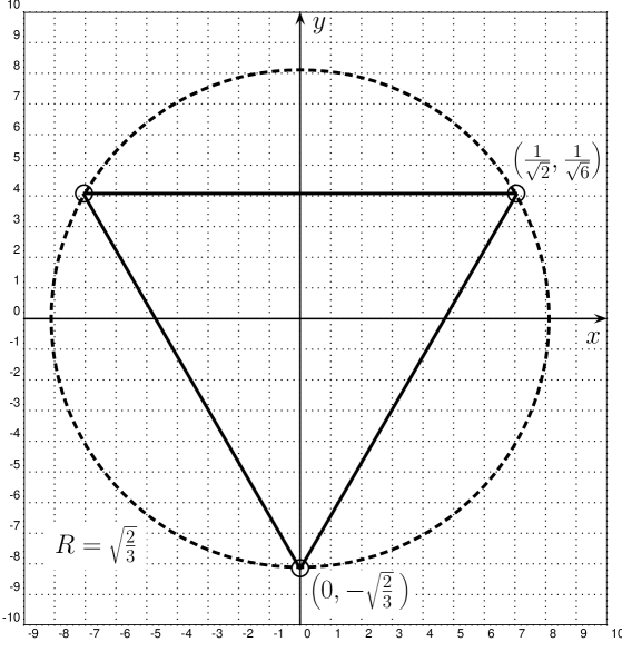
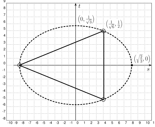
Figure 1: Type I (a) left and type II (b ) right. Allowed states lie on the solid lines and inside the triangles. Small circles – pure states. The grid unit corresponds to actual value equal to $0.1$.

Type I corresponds to only one pair of parameters, that is to $(s,t)=(x,y)$. Then, requirements (1fgracaubfbjcc) and (1fgracaubfbjcg) translate into the following ones

$$\bigl{|}{\vec{\bf{V}}}\bigr{|}^{2}=x^{2}+y^{2}\leq\frac{2}{3},$$ (1fgracaubfbjcha)

$$F(x,y)=\frac{1}{9}-\frac{x^{2}+y^{2}}{2}+\frac{3x^{2}y-y^{3}}{\sqrt{6}}\geq 0.$$ (1fgracaubfbjchb)

Requirement (1fgracaubfbjcha) restricts allowed values of $x$, $y$ to the circle of the radius $R=\sqrt{2/3}$ (dashed line). Then (1fgracaubfbjchb) implies that the allowed points must lie within or on the triangle indicated by solid lines in Figure 1. We also note that for this type there are three possible pure states $(\pm 1/\sqrt{2},1/\sqrt{6})$ and $(0,-\sqrt{2/3})$. They are indicated by small circles in Figure 1.

6.2.2 Type II

Type II has two representatives $(s,t)=(y,\alpha_{2}),(y,\beta_{2})$. Then relations (1fgracaubfbjcc) and (1fgracaubfbjcg) give

$$\bigl{|}{\vec{\bf{V}}}\bigr{|}^{2}=s^{2}+2\,t^{2}\leq\frac{2}{3},$$ (1fgracaubfbjchcia)

$$F(s,t)=\frac{1}{9}-\frac{s^{2}}{2}-t^{2}+\frac{6t^{2}s-s^{3}}{\sqrt{6}}\geq 0.$$ (1fgracaubfbjchcib)

Inequality (1fgracaubfbjchcia) places the allowed values of parameters on and inside the ellipse with semi-axes of lengths $\sqrt{2/3}$ and $\sqrt{1/3}$ (dashed line in Figure 1 (right)). Inequality (1fgracaubfbjchcib) restricts $s$ and $t$ to the triangle drawn with solid lines in Figure 1 (right). There are also three pure states $(\sqrt{1/6},\pm\sqrt{1/2})$ and $(-\sqrt{2/3},0)$.

6.2.3 Type III

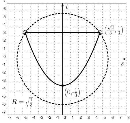
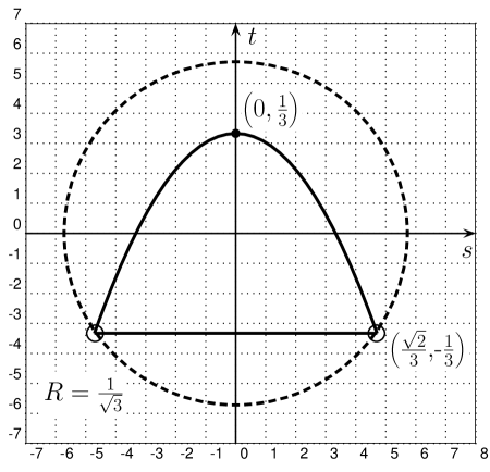
Figure 2: Type III (a) left and type IV (b) right. Allowed states lie on the solid lines and inside the region restricted by a horizontal straight lines and parabolas. Small circles – pure states. The grid unit, as previously, corresponds to actual value equal to $0.1$

Type III is specified by two cases $(s,t)=(a,\alpha_{2}),(\beta_{1},\alpha_{2})$. Then from (1fgracaubfbjcc) and (1fgracaubfbjcg) we get

$$\bigl{|}{\vec{\bf{V}}}\bigr{|}^{2}=2(s^{2}+t^{2})\leq\frac{2}{3},$$ (1fgracaubfbjchcicja)

$$F(s,t)=\frac{1}{9}-s^{2}-t^{2}+3s^{2}t\geq 0.$$ (1fgracaubfbjchcicjb)

The first condition gives allowed values of parameters $s$ and $t$ within a circle of radius $R=\sqrt{1/3}$ (dashed line in Figure 2 (left). The requirement (1fgracaubfbjchcicjb) restricts the values of $s$, $t$ to a region below the straight line $t=1/3$ and above the parabola $t=3s^{2}-1/3$. This region is indicated by a solid line in Figure 2 (left). This type allows for two pure states $(\pm\sqrt{2}/3,1/3)$ which are denoted by small circles.

6.2.4 Type IV

Type IV is similar to the previous one. In this case we also have two cases $(s,t)=(b,\alpha_{2}),(\alpha_{1},\alpha_{2})$. Then from (1fgracaubfbjcc) and (1fgracaubfbjcg) it follows that

$$\bigl{|}{\vec{\bf{V}}}\bigr{|}^{2}=2(s^{2}+t^{2})\leq\frac{2}{3},$$ (1fgracaubfbjchcicjcka)

$$F(s,t)=\frac{1}{9}-s^{2}-t^{2}-3s^{2}t\geq 0.$$ (1fgracaubfbjchcicjckb)

The imposed conditions are thus similar. Only now, inequality (1fgracaubfbjchcicjckb) implies that the allowed points are above the straight line $t=-1/3$ and below the parabola $t=-3s^{2}+1/3$ drawn as solid lines in Figure 2 (right). Two pure states correspond to points $(\pm\sqrt{2}/3,-1/3)$.

6.2.5 Type V

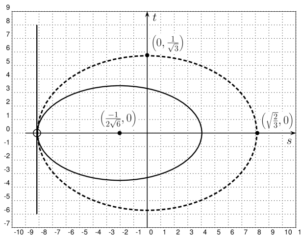
Figure 3: Type V. Allowed states lie on and inside the solid ellipse. Small circles – pure states. The grid unit equals to $0.1$

Type V has four representatives, namely $(s,t)=(y,a),(y,b),(y,\alpha_{1}),$ $(y,\beta_{1})$. Next, from (1fgracaubfbjcc) with (1fgracaubfbjcg) we have

$$\bigl{|}{\vec{\bf{V}}}\bigr{|}^{2}=s^{2}+2t^{2}\leq\frac{2}{3},$$ (1fgracaubfbjchcicjckcla)

$$F(s,t)=\frac{1}{9}-\frac{s^{2}}{2}-t^{2}-\frac{3t^{2}s+s^{3}}{\sqrt{6}}\geq 0.$$ (1fgracaubfbjchcicjckclb)

The first requirement puts the allowed points within an ellipse with semi-axes of lengths $\sqrt{2/3}$ and $\sqrt{1/3}$. Condition (1fgracaubfbjchcicjckclb) implies that the values of $s$ and $t$ are to the right of the straight line $s=-\sqrt{2/3}$ and within an ellipse the center of which is shifted to the point $(-1/2\sqrt{6},0)$. Semi-axes of this ellipse are equal to $\sqrt{3/8}$ and $\sqrt{1/8}$. So, the allowed points are within (and on) the smaller ellipse which is drawn with a solid line in Figure 3. Here, there is only one pure state at the point $(-\sqrt{2/3},0)$ indicated by a small circle.

6.2.6 Type VI

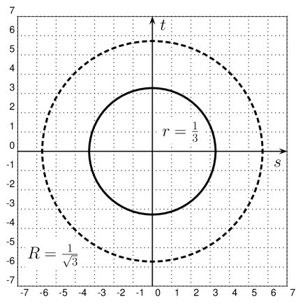
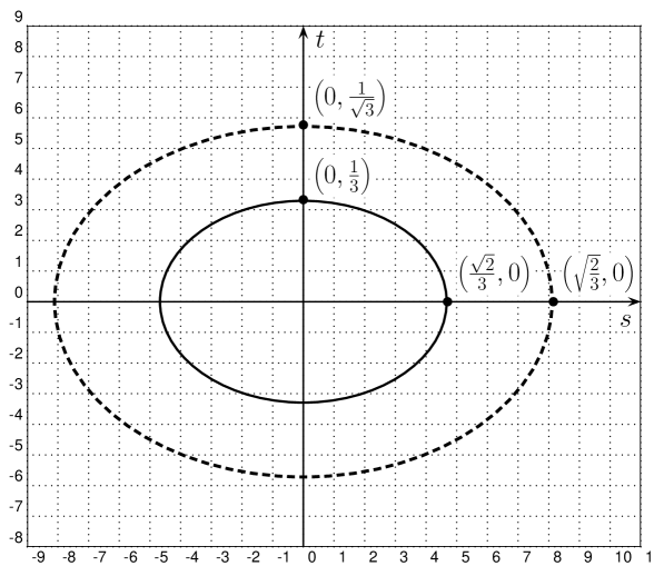
Figure 4: Type VI (left) and type VII (right). The allowed states lie on and within the solid curves. There are no pure states. The grid unit equals $0.1$, as always.

This type is most numerous, it is specified by 11 cases. They are $(s,t)=(a,b),(a,\alpha_{1}),(a,\beta_{1}),(a,\beta_{2}),(b,\alpha_{1}),(b,\beta_{1}),(b,\beta_{2}),(\alpha_{1},\beta_{1}),(\alpha_{1},\beta_{2}),(\beta_{1},\beta_{2}),$ $(\alpha_{2},\beta_{2})$. Then, requirements (1fgracaubfbjcc) and (1fgracaubfbjcg) yield

$$\bigl{|}{\vec{\bf{V}}}\bigr{|}^{2}=2(s^{2}+t^{2})\leq\frac{2}{3},$$ (1fgracaubfbjchcicjckclcma)

$$F(s,t)=\frac{1}{9}-s^{2}-t^{2}\geq 0,$$ (1fgracaubfbjchcicjckclcmb)

because in this case we find $T_{3}=0$. Both conditions specify circles. Inequality (1fgracaubfbjchcicjckclcma) gives a circle with radius $R=\sqrt{1/3}$ while (1fgracaubfbjchcicjckclcmb) yields $r=\sqrt{1/3}$. The smaller circle (more restrictive) is drawn solid in Figure 4. No pure states are allowed here.

6.2.7 type VII

The last type is given by 6 pairs, that is by $(s,t)=(x,a),$ $(x,b),(x,\alpha_{1}),$ $(x,\beta_{1}),(x,\alpha_{2}),$ $(x,\beta_{2})$. Then relations (1fgracaubfbjcc) and (1fgracaubfbjcg) give the requirements

$$\bigl{|}{\vec{\bf{V}}}\bigr{|}^{2}=s^{2}+2t^{2}\leq\frac{2}{3},$$ (1fgracaubfbjchcicjckclcmcna)

$$F(s,t)=\frac{1}{9}-\frac{s^{2}}{2}-t^{2}\geq 0,$$ (1fgracaubfbjchcicjckclcmcnb)

since in this case we also have $T_{3}=0$. Condition (1fgracaubfbjchcicjckclcmcna) restricts the allowed values of $s$ and $t$ to an ellipse with semi-axes equal to $\sqrt{2/3}$ and $\sqrt{1/3}$. The second condition restricts the allowed points to within and on an ellipse with semi-axes $\sqrt{2}/3$ and $1/3$. The smaller ellipse is drawn solid in Figure 4. As in the previous type there are no pure states.

6.3 Features common to all seven types

All discussed types are characterized by two-parameter behaviour of $|{\vec{\bf{V}}}|^{2}$ and $F(s,t)$, the latter being proportional to $\det\hat{\rho}$ (up to a factor of $1/3$). In all considered cases requirement $F(s,t)\geq 0$ is more restrictive than the condition imposed upon the length of the generalized Bloch vector ${\vec{\bf{V}}}$. That confirms the idea that the set of all density matrices is a proper subset of the hyperball determined by requiring that $|{\vec{\bf{V}}}|^{2}\leq 2/3$.

The allowed values of parameters lie on and inside the solid contours which correspond to $F(s,t)=0$. Since for pure states we have $|{\vec{\bf{V}}}|^{2}=2/3$ and $\det\hat{\rho}=0$ it is not surprising that pure states are situated at the extremal points of solid contours.

Inside these contours $F(s,t)$ is obviously positive and for all cases attains its maximal value equal to $1/9$ at the point $(0,0)$ which corresponds to ${\vec{\bf{V}}}=0$, that is to a maximally mixed state.

7 Final remarks

We have presented and discussed the representation of the $N\times N$ dimensional density matrix in terms of polarization operators ${\!\mbox{ {T}}}_{LM}(j)$. This idea is not entirely new (see, for example [7, 8]), but the usefulness of this expansion seems to justify our recollection of known facts. On the other hand, we have discussed the important issue of positivity which seems not, in the context of polarization operators, to be considered in the literature known to us.

Usefulness of the presented approach, as it seems to us, stems mainly from the fact that polarization operators are expressed in terms of quantities well-known from the quantum theory of angular momentum. Connection with this theory greatly facilitates all considerations and allows derivation of expressions valid for any $N=2j+1$. For example, it is straightforward to find commutators, products, traces over products, etc. This can be done analytically, but also with the aid of computer programs allowing symbolic mathematics. These possibilities seem to indicate that the discussed approach is indeed useful in practice.

Polarization operators ${\!\mbox{ {T}}}_{LM}(j)$ constitute a basis in the space of $N\times N$ dimensional operators. Hence, the density operator can be expanded as in (1fgracai). This establishes a relationship between $N\times N$ dimensional density matrices and ${\vec{\bf{V}}}$’s – generalized Bloch vectors. Expansion (1fgracai) automatically ensures proper normalization of the density operator. This is due to the fact that polarization operators are traceless. Next, requirement of hermiticity implies that complex components $V_{LM}^{\ast}=(-1)^{M}V_{L-M}$ which reduces the number of independent real parameters to $N^{2}-1$ and fixes the dimension of the space of generalized Bloch vectors.

Density operator must be not only normalized and hermitian but also positive. This problem seems not to be discussed earlier a in terms of polarization operators. We have done that and presented the formalism allowing one to check whether the positivity conditions are met by a given hermitian and normalized matrix. Successive positivity requirements (that is inequalities $S^{(N)}_{k}\geq 0$ for $k=2,3,\ldots,N$) are derived for any $N$. These requirements specify and restrict the space of generalized Bloch vectors which represent true density matrices. Expressions (1fgracaube) together with (1fgra) allow computation of the quantities $T_{m}=\Tr\{({\vec{\bf{V}}}\cdot{\vec{\bf{{\!\mbox{ {T}}}}}})^{m}\}$ which, in turn, are used to compute coefficients $S^{(N)}_{k}$ as in (1fgracaubfbi). In particular, requirement $S^{(N)}_{2}\geq 0$ entails $\Tr\{\hat{\rho}^{2}\}\leq 1$ which, in terms of Bloch vector yields $|{\vec{\bf{V}}}|^{2}\leq(N-1)/N$. So, all vectors ${\vec{\bf{V}}}$ lie within a $N^{2}-1$ dimensional hyperball of radius equal to $\sqrt{(N-1)/N}$. However, further conditions $S^{(N)}_{k}\geq 0$ (for $k\geq 3$) severely restrict the set of allowed Bloch vectors. This set is a proper subset of the mentioned hyperball and it possesses quite a complicated structure. In the two previous sections we employed the presented procedure to a qubit ($N=2$) and to qutrit ($N=3$). The former is quite simple. On the other hand analysis of a qutrit gives support to all above given remarks.

The employed representation of the density operator seems to be quite useful. We feel that we have shown that it can successfully be used to investigate issues which were not studied earlier and which seem to be of contemporary interest. Moreover, the procedure to investigate positivity is valid for any $N$.

Finally, we would like to indicate some possibilities which probably deserve further attention. Polarization operators are spherical irreducible tensors [7]. Therefore, their tensor products preserve their character. This fact seems to be promising in the investigations of entangled states. We hope that this can provide new insights into the structure and geometry of entangled states. Moreover, as indicated by Biederharn and Louck [8], polarization operators consitute just another (non-standard) set of $SU(N)$ generators. This set is endowed with an interesting stucture as it follows from careful inspection of the structure constants in (1fgry). Investigation based upon this fact go beyond the scope of this work, but seem to be an interesting subject for future studies of the space of allowed generalized Bloch vectors and therefore of the geometry of the space of density operators.

We end this paper with the hope that the revitalized expansion of the density operator in terms of polarization operators will prove useful in other investigations. The presented discussion of the correspondence between density operators and generalized Bloch vectors (especally in the light of requirement of positivity) is applicable to any dimension. The quantities appearing here are strongly connected with angular momentum theory and thereby well-known. This, in our minds, indicates that the representation discussed here may be more practical then the ”standard” one.

References

References

- [1] Keyl M 2002 Phys. Rep. 369 431–548
- [2] Kimura G 2002 Phys. Let. A 314 339–349
- [3] Byrd M S Khaneja N 2003 Phys. Rev. A 68 062322
- [4] Jakóbczyk L Siennicki M 2001 Phys. Lett. A 286 383-390
- [5] Jaegger G Sergienko A V Saleh B E A and Teich M C 2003 Phys. Rev. A 68 022318
- [6] Gantmacher F R 1959 1960 1977 Theory of Matrices (New York: Chelsea Publishing Company)
-
[7]
Varshalovich D A Moskalev A N and Khersonskii W K 1975
Quantum Theory of Angular Momentum
(Leningrad: Nauka, Leningrad)
(Russian version is available tu us)
Varshalovich D A Moskalev A N and Khersonskii W K 1988 Quantum Theory of Angular Momentum (Singapore: World Scientific) - [8] Biedenharn L C Louck J D 1981 Angular momentum in Quantum Physics. Theory and Application (Boston: Addison-Wesley, Reading)
- [9] Tilma T Sudarshan ECG 2002 J. Phys. A: Math. Gen.35 10467–501
- [10] Alicki R Lendi K 1987 Quantum Dynamical Semigroups and Applications (New York: Springer)
- [11] Cohen-Tannoudji C Dupont-Roc J and Grynberg G 1992 Atom-Photon Interactions (New York: Wiley)
- [12] Puri, R R 2001 Mathematical Methods of Quantum Optics (New York: Springer)