Cooperative spin decoherence and population transfer

Abstract

An ensemble of multilevel atoms is a good candidate for a quantum information storage device. The information is encrypted in the collective ground state atomic coherence, which, in the absence of external excitation, is decoupled from the vacuum and therefore decoherence free. However, in the process of manipulation of atoms with light pulses (writing, reading), one inadvertently introduces a coupling to the environment, i.e. a source of decoherence. The dissipation process is often treated as an independent process for each atom in the ensemble, an approach which fails at large atomic optical depths where cooperative effects must be taken into account. In this paper, the cooperative behavior of spin decoherence and population transfer for a system of two, driven multilevel-atoms is studied. Not surprisingly, an enhancement in the decoherence rate is found, when the atoms are separated by a distance that is small compared to an optical wavelength; however, it is found that this rate increases even further for somewhat larger separations for atoms aligned along the direction of the driving field’s propagation vector. A treatment of the cooperative modification of optical pumping rates and an effect of polarization swapping between atoms is also discussed, lending additional insight into the origin of the collective decay.

year number number identifier Date text]date

LABEL:FirstPage1 LABEL:LastPage#1

I Introduction

A system of atoms interacting with a common reservoir (the electromagnetic vacuum) is often treated using an assumption of independent dissipation rates for the atoms. This is a valid assumption for the case when the interatomic distances are large (compared to an optical wavelength); however, when the distances between atoms become smaller or comparable to an optical wavelength, the mode structure around one atom is changed due to the presence of other atoms located in its immediate vicinity, and the decay rates are modified. Equivalently, the radiation emitted by one atom can be scattered off the second atom, thus changing the radiative properties of the system. As a consequence, the radiative decay of the ensemble must be viewed as a cooperative effect. A quantitative analysis of cooperative effects was given by Dicke dicke for an ensemble of two-level systems confined to a spherical volume whose radius is much smaller than an optical wavelength. For such a system, the collective decay rate can be increased by a factor proportional to the number of atoms in the ensemble. Further investigations extend the treatment to arbitrary interatomic distances, although the calculations become more complex. Formalisms for the treatment of cooperative spontaneous emission and resonance fluorescence from a system of many atoms have been developed ernst-stehle ; lehmberg1 ; agarwal ; eberly ; walls , and have been applied to a system of two two-level atoms lehmberg2 ; ficek ; richter .

Cooperative decay in multilevel atomic systems has yet to be treated in detail. A multilevel atom has properties not possessed by a two-level atom: for example, it can store information in superpositions of ground state magnetic sublevels. Such ensembles are extensively discussed in the literature as convenient systems for information storage or large scale entanglement generation entanglement . In particular, pencil-shaped media have been used for the generation of spin squeezed and Schrodinger cat states, in the context of continuous measurement of a scattered field pencil-entanglement . In such schemes, the coupling to the vacuum has a two-fold function: on one hand it gives rise to the signal while, on the other hand, it leads to an irreversible leakage of information from the system to the environment. In treating the losses due to spontaneous emission, the above mentioned assumption of independent atoms is generally used, which is a sound assumption as long as the atomic density is low. However, optimal results (e.g. strong entanglement) are found in the regime of resonant optical depths greater than unity, a regime in which pencil-shaped media of two-level atoms exhibit superradiant behavior pencil . Even if the dynamics of a collection of multilevel atoms might be substantially different from that of the two-level ensemble, the validity of the independent spontaneous emission regime is questionable.

We proceed in the present publication with an analysis of cooperative effects in a system of two, four-level atoms. This provides the starting point for an extension to many atom systems, while it also addresses the non-trivial question of the importance of cooperative decoherence in a simple quantum information system of two qubits. The calculations are performed for a $J=1/2\rightarrow J^{\prime}=1/2$ transition irradiated with a monochromatic, off-resonant, $\sigma_{+}$ polarized, classical laser field. The collective decoherence of an initial equal superposition of ground sublevels ($x$ polarized atomic state) is obtained for arbitrary interatomic separations and compared with that of atoms independently coupled to the reservoir. In addition, the transfer of population from a $z$ polarized atomic state with both atoms in one of the ground sublevels to another $z$ polarized state with both atoms in the other sublevel, is analyzed. A polarization swap effect is also discussed, where an $x$ polarized atom induces $x$ coherence in a neighboring atom footnote .

The paper is organized as follows: in Sec. II the theoretical method used is described. In Sec. III analytical solutions for the case of close atoms are obtained. Numerical solutions for arbitrary separations are discussed and plotted in Sec. IV. In Sec. V the polarization swap effect for arbitrary separations is discussed, while Sec. VI contains some conclusions.

II Theory

As indicated in Fig. 1(a), the two atoms (having natural frequency $\omega_{0}$) are located at the origin, $\mathbf{R}_{1}=0$, and at $\mathbf{R}_{2}=\mathbf{R}_{21}$, respectively. The traveling wave driving field propagates in the positive $z$ direction with wave vector $\mathbf{k}$, frequency $\Omega$ (detuned from $\omega_{0}~{}$by $\Delta$), and circular polarization $\sigma_{+}$.

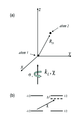
Figure 1: (a) The classical field is propagating along the $z$ axis, driving the two atoms, located at the origin $R_{1}=0$ and at $R_{2}=R_{21}$, respectively. (b) Internal structure of a single atom.     

Denoting the $4$ states of a single atom with $\left|\downarrow\right\rangle$ (ground, $m_{\downarrow~{}}=-1/2$ eigenvalue), $\left|\uparrow\right\rangle$ (ground, $m_{\uparrow~{}}=1/2$ eigenvalue), $\left|\beta\right\rangle$ (excited, $m_{\beta~{}}=-1/2$ eigenvalue) and $\left|\alpha\right\rangle$ (excited, $m_{\alpha~{}}=1/2$ eigenvalue), the classical field drives the $\left|\downarrow\right\rangle\rightarrow$ $\left|\alpha\right\rangle$ transitions. The Hamiltonian for the system (composed of the two atoms indexed with $i$, where $i=1,2$) is a sum of the free Hamiltonian ($H_{0}$), the classical field-atom interaction Hamiltonian ($V_{c}$) and quantized bath-atom interaction Hamiltonian ($V_{q}$) given by:

$$H_{0~{}} =\underset{i=1,2}{{\textstyle\sum}}\hbar\omega_{0}\left[\left|\alpha\right\rangle_{i}\left\langle\alpha\right|_{i~{}}+\left|\beta\right\rangle_{i}\left\langle\beta\right|_{i}\right]+\underset{\mathbf{k},\lambda}{{\textstyle\sum}}\hbar\omega_{k}a_{\mathbf{k},\lambda}^{\dagger}a_{\mathbf{k},\lambda~{}},$$ (1)

$$V_{c~{}} =\underset{i=1,2}{{\textstyle\sum}}\hbar\chi\left[\left|\alpha\right\rangle_{i}\left\langle\downarrow\right|_{i~{}}e^{i\mathbf{k}_{L}\mathbf{\cdot R}_{i~{}}}e^{-i\Omega t}+\left|\downarrow\right\rangle_{i}\left\langle\alpha\right|_{i~{}}e^{-i\mathbf{k}_{L}\mathbf{\cdot R}_{i~{}}}e^{i\Omega t}\right],$$

$$V_{q~{}} =\underset{i=1,2}{{\textstyle\sum}}\left[\underset{j=\downarrow,\uparrow}{{\textstyle\sum}}\underset{j^{\prime}=\beta,\alpha}{{\textstyle\sum}}\underset{\mathbf{k},\lambda}{{\textstyle\sum}}\hbar\left[g_{\mathbf{k},\lambda~{}}^{jj^{\prime}}\left|j\right\rangle_{i}\left\langle j^{\prime}\right|_{i~{}}a_{\mathbf{k},\lambda~{}}^{\dagger}e^{-i\mathbf{k\cdot R}_{i~{}}}+\left(g_{\mathbf{k},\lambda~{}}^{jj^{\prime}}\right)^{\ast}\left|j^{\prime}\right\rangle_{i}\left\langle j\right|_{i~{}}a_{\mathbf{k},\lambda~{}}e^{i\mathbf{k\cdot R}_{i~{}}}\right]\right].$$

As usual, the field is quantized in a volume $\mathcal{V}$ and is described by the creation and annihilation operators $a_{\mathbf{k},\lambda~{}}^{\dagger}$and $a_{\mathbf{k},\lambda}$, corresponding to modes with wave vector $\mathbf{k}$ and polarization $\lambda$. The atomic dipole moment $\mathbf{d}$ (the same for both atoms) couples to both the classical and quantized fields. The cw driving field at the position of the atoms ($\mathbf{R}_{i~{}}$ for $i=1,2$) is expressed as $\mathbf{E}\left(\mathbf{R},t\right)\mathbf{=}\frac{1}{2}\left[E_{0~{}}e^{i\mathbf{k}_{L~{}}\mathbf{\cdot R}_{i~{}}}e^{-i\Omega t}+cc\right]\widehat{\mathbf{\epsilon}}_{+~{}}$. The classical part of the interaction contains the Rabi frequency defined as:

$$\chi=\frac{d_{+}E_{0}}{2\hbar},$$ (2)

where $d_{+}$ is the matrix element $d_{+}=\left\langle\alpha\right|\mathbf{d}\cdot\widehat{\mathbf{\epsilon}}_{+}\left|\downarrow\right\rangle$; the interaction with the quantum vacuum has an associated coupling strength

$$g_{\mathbf{k},\lambda~{}}^{jj^{\prime}}=-i\left(\frac{\omega_{k~{}}}{2\epsilon_{0}\hbar\mathcal{V}}\right)^{1/2}d_{\mathbf{k},\lambda~{}}^{jj^{\prime}}$$ (3)

proportional to the dipole matrix element in the direction of the unit polarization vector $d_{\mathbf{k},\lambda~{}}^{jj^{\prime}}=\left\langle j\right|\mathbf{d}\cdot\widehat{\mathbf{\epsilon}}_{\mathbf{k},\lambda~{}}\left|j^{\prime}\right\rangle$.

The quantities that are relevant in what follows are the collective coherence operator

$$P_{\downarrow\uparrow~{}}=\underset{i=1,2}{{\textstyle\sum}}\left|\downarrow\right\rangle_{i}\left\langle\uparrow\right|_{i~{}}$$ (4)

and the normalized population operator

$$P_{\uparrow\uparrow~{}}=\frac{1}{2}\underset{i=1,2}{{\textstyle\sum}}\left|\uparrow\right\rangle_{i}\left\langle\uparrow\right|_{i~{}}.$$ (5)

The derivation of the time evolution of the expectation values of these two operators is the goal of our calculations. They can expressed in terms of density matrix elements as

$$\left\langle P_{\downarrow\uparrow~{}}\right\rangle =\rho_{\uparrow\uparrow;\downarrow\uparrow~{}}+\rho_{\uparrow\downarrow;\downarrow\downarrow~{}}+\rho_{\uparrow\uparrow;\uparrow\downarrow~{}}+\rho_{\downarrow\uparrow;\downarrow\downarrow~{}},$$ (6)

$$\left\langle P_{\uparrow\uparrow~{}}\right\rangle =\frac{1}{2}\left(2\rho_{\uparrow\uparrow;\uparrow\uparrow~{}}+\rho_{\uparrow\downarrow;\uparrow\downarrow~{}}+\rho_{\downarrow\uparrow;\downarrow\uparrow~{}}\right).$$

  We consider two problems: first, one with both atoms prepared initially in a superposition of ground states with maximum coherence $\frac{1}{\sqrt{2}}\left(\left|\downarrow\right\rangle+\left|\uparrow\right\rangle\right)$ (collective coherence equal to $1$) and, second, one where the population is transferred from the state with both atoms in the $\left|\downarrow\right\rangle$ state to the one with both atoms in the $\left|\uparrow\right\rangle$ state.

Qualitative (and some quantitative) details of the calculations are described in the following. The subspace of interest in which the collective operators defined above act (henceforth named the ground subspace) is of dimension $4$ and it is spanned by state vectors containing the ground substates of the two atoms ( $\left|\downarrow\downarrow\right\rangle$,$\left|\downarrow\uparrow\right\rangle$, $\left|\uparrow\downarrow\right\rangle$ and $\left|\uparrow\uparrow\right\rangle$). A set of $16$ density matrix equations completely describes the dynamics of this space. However, the ground subspace is coupled to the ground-excited subspace of dimension $8$ (containing states with one excitation as for example $\left|\downarrow\alpha\right\rangle$) through the classical field. This is, in its turn, coupled to the excited subspace of dimension $4$ (containing states of two excitations like $\left|\alpha\alpha\right\rangle$) which can decay back to the ground states. In a density operator approach, a total of $256$ density matrix elements coupled to each other come into play, which makes the task at hand extremely complex.

Some simplifications are possible. First, terms occurring in the evolution of the ground state density matrix elements are separated into in-terms (due to spontaneous emission from upper states) and out-terms (driving terms due to the presence of the classical field), and these terms are treated separately. Second, an amplitude rather than a density matrix approach is sufficient to obtain expressions for the excited-ground and excited subspace density matrix elements which enter the equations. The procedure is described in Appendix B where it is applied to the derivation of the decoherence and population transfer rate for a single 4-level atom. The treatment is perturbative in the sense that excited state populations are assumed to be negligibly small, as in many treatments of optical pumping.

The states coupled by the fields in this approximation are denoted by $\left|\mu^{\prime}\nu\right\rangle$, $\left|\mu\nu^{\prime}\right\rangle$ and $\left|\mu\nu\right\rangle$ where the convention used is that the prime indicates excited states ($\alpha$ or $\beta$), while the unprimed symbols indicate ground states ($\uparrow$ or $\downarrow$). By eliminating the intermediate states involving the radiation field (procedure outlined in Refs. hao-berman ; berman-milonni ), one can obtain the following coupled equations of motion for the state amplitudes containing one excitation ($b_{\mu\nu^{\prime}}$ and $b_{\mu^{\prime}\nu}$), in an interaction picture:

$$\overset{\cdot}{b}_{\mu^{\prime}\nu~{}} =-\gamma b_{\mu^{\prime}\nu~{}}-\gamma\underset{\mu,\nu^{\prime}}{{\textstyle\sum}}G_{m_{\mu^{\prime}}-m_{\mu~{}};m_{\nu^{\prime}}-m_{\nu~{}}}(\mathbf{R}_{21})\left\{m_{\mu~{}},m_{\mu^{\prime}~{}}\right\}\left\{m_{\nu~{}},m_{\nu^{\prime}}\right\}b_{\mu\nu^{\prime}~{}}$$ (7)

$$-i\Delta b_{\mu^{\prime}\nu~{}}+i\chi e^{i\mathbf{k}_{L}\mathbf{\cdot R}_{1~{}}}b_{\downarrow\nu~{}}\delta_{m_{\mu^{\prime}},1/2~{}},$$

$$\overset{\cdot}{b}_{\mu\nu^{\prime}~{}} =-\gamma b_{\mu\nu^{\prime}~{}}-\gamma\underset{\mu,\nu^{\prime}}{{\textstyle\sum}}G_{m_{\mu~{}}-m_{\mu^{\prime}};m_{\nu~{}}-m_{\nu^{\prime}}}(\mathbf{R}_{12})\left\{m_{\mu^{\prime}~{}},m_{\mu~{}}\right\}\left\{m_{\nu^{\prime}~{}},m_{\nu~{}}\right\}b_{\mu^{\prime}\nu~{}}$$

$$-i\Delta b_{\mu\nu^{\prime}~{}}+i\chi e^{i\mathbf{k}_{L}\mathbf{\cdot R}_{2~{}}~{}}b_{\mu\downarrow~{}}\delta_{1/2,m_{\nu^{\prime}}~{}}.$$

In the equation above for $\overset{\cdot}{b}_{\mu^{\prime}\nu}$, the first term on the right-hand side is the decay (at a rate $\gamma$ equal to half the excited state population decay rate) of the excited state amplitude of an atom independently coupled to the quantum vacuum. The second term contains a propagator $G_{m_{\mu^{\prime}}-m_{\mu};m_{\nu^{\prime}}-m_{\nu}}\left(\mathbf{R}_{21}\right)$ which includes the effects of the radiation exchange between atoms: an atom makes a transition from state $\nu^{\prime}$ (quantum number $m_{\nu^{\prime}}$) to state $\nu$ which is accompanied by a transition in the other atom ($\mu$ to $\mu^{\prime}$). The real part of $G$ gives a contribution to the decay rate that varies from $1$, for maximum cooperation between atoms when their separation is much less than $\lambda$, to $0$, when no exchange of radiation between atoms is present (infinite separation). The imaginary part leads to a shift in energy (which adds to $\Delta$ in the equations above) and varies from $0$ (large separation) to infinity when the atoms are in the same location. If the minimum interatomic separation is small but finite, the shift can always be kept small compared to the detuning and can be neglected. The explicit expressions for the propagators involved in this problem are given in Appendix A. The geometrical information on the radiation exchange is contained in the Clebsch-Gordan coefficients $\left\{m,m^{\prime}\right\}\equiv\left\langle 1/2,1/2;m,m^{\prime}|1,m-m^{\prime}\right\rangle$. The last two terms in the right-hand side arise from driving field induced transitions and from the off-resonant nature of the interaction.

To calculate the out-terms, we note that, as a result of the driving field, ground state amplitudes ($b_{\mu\nu~{}}$) are coupled to excited state amplitudes via

$$\overset{\cdot}{b}_{\mu\nu~{}}=i\chi\left[e^{-i\mathbf{k}_{L}\mathbf{\cdot R}_{1~{}}}b_{\alpha\nu~{}}\delta_{-1/2,m_{\mu~{}}~{}}+e^{-i\mathbf{k}_{L}\mathbf{\cdot R}_{2~{}}}b_{\mu\alpha~{}}\delta_{-1/2,m_{\nu~{}}~{}}\right].$$ (8)

As a result one finds

$$\overset{\cdot}{\rho}_{\mu\nu;mn}^{out} =\overset{\cdot}{b}_{\mu\nu~{}}b_{mn~{}}^{\ast}+b_{\mu\nu~{}}\overset{\cdot}{b}_{mn~{}~{}}^{\ast}=\left[i\chi e^{-i\mathbf{k}_{L}\mathbf{\cdot R}_{1~{}}}b_{\alpha\nu~{}}\delta_{-1/2,m_{\mu~{}}~{}}+e^{-i\mathbf{k}_{L}\mathbf{\cdot R}_{2~{}}}b_{\mu\alpha~{}}\delta_{-1/2,m_{\nu~{}}~{}}\right]b_{mn~{}}^{\ast}+$$ (9)

$$+b_{\mu\nu~{}}\left[i\chi e^{-i\mathbf{k}_{L}\mathbf{\cdot R}_{1~{}}}b_{\alpha n~{}}\delta_{-1/2,m_{m~{}}~{}}+e^{-i\mathbf{k}_{L}\mathbf{\cdot R}_{2~{}}}b_{m\alpha~{}}\delta_{-1/2,m_{n~{}}~{}}\right].$$

The system of equations (Eqs. (7)) is solved for the $8$ amplitudes $b_{\mu^{\prime}\nu~{}}$ and $b_{\mu\nu^{\prime}~{}}$ as functions of the $4$ ground state amplitudes $b_{\mu\nu~{}}$; these expressions are replaced in the above equation and with the identification $b_{\mu\nu~{}}b_{mn~{}}^{\ast}\rightarrow\rho_{\mu\nu;mn~{}}$, the rate equations for $\overset{\cdot}{\rho}_{\mu\nu;mn}^{out}$ are obtained in terms of the $16$ density matrix elements $\rho_{\mu\nu;mn~{}}$(with $\mu,\nu,m,n=\downarrow,\uparrow$).

Next, repopulation from the upper states to the lower states is taken into account (in-terms)

$$\overset{\cdot}{\rho}_{mn;\mu\nu}^{in} =\underset{m^{\prime},\mu^{\prime}}{{\textstyle\sum}}\Gamma_{m\mu~{}}^{m^{\prime}\mu^{\prime}}\rho_{m^{\prime}n;\mu^{\prime}\nu~{}~{}}+\underset{n^{\prime},\nu^{\prime}}{{\textstyle\sum}}\Gamma_{n\nu~{}}^{n^{\prime}\nu^{\prime}}\rho_{mn^{\prime};\mu\nu^{\prime}~{}}+$$ (10)

$$(2\gamma)\underset{m^{\prime},\nu^{\prime}}{{\textstyle\sum}}G_{m_{\nu^{\prime}}-m_{\nu};m_{m^{\prime}}-m_{m}}(\mathbf{R}_{21})\left\{m_{m~{}},m_{m^{\prime}~{}}\right\}\left\{m_{\nu~{}},m_{\nu^{\prime}~{}}\right\}\rho_{m^{\prime}n;\mu\nu^{\prime}~{}}+$$

$$(2\gamma)\underset{m^{\prime},\nu^{\prime}}{{\textstyle\sum}}G_{m_{\mu^{\prime}}-m_{\mu};m_{n^{\prime}}-m_{n}}(\mathbf{R}_{21})\left\{m_{\mu},m_{\mu^{\prime}}\right\}\left\{m_{n},m_{n^{\prime}}\right\}\rho_{mn^{\prime};\mu^{\prime}\nu}~{},$$ (11)

where

$$\Gamma_{ab~{}}^{a^{\prime}b^{\prime}}=(2\gamma)\left\{m_{a~{}},m_{a^{\prime}}\right\}\left\{m_{b~{}},m_{b^{\prime}}\right\}\delta_{m_{a^{\prime}}-m_{a~{}},m_{b^{\prime}~{}}-m_{b~{}}~{}}.$$ (12)

Note that some coherence is returned to the ground state as a result of the ”in terms”. The derivation of the terms in the right-hand side of Eq. (10) is done by tracing over the field states with one-photon occupation number, a procedure which has been used in the case of single multilevel atoms [see for example Ref. in-terms ]. The first two terms describe repopulation and recoherence of the ground manifold from the excited state manifold in a single atom. Cross coupling between atoms is reflected in the next two terms. Using again the solutions of Eqs. (7), the right-hand side of the in-term equations can be expressed in terms of ground state density matrix elements. A complete system of $16$ linear equations is thus obtained by adding the in-term to the out-term contributions.

III Small Separation ($\mathbf{R}_{21}\ll\lambda$)

In this limit, owing to angular momentum conservation rules, the propagators $G_{ij~{}}$ vanish except for $i=j$. A few photon exchange processes between atoms are illustrated in Fig. 2(c), along with their accompanying propagators. Notice that due to momentum conservation the polarization of the emitted photon matches the polarization of the absorbed photon. Taking as an example the transfer of excitation from atom $1$ in state $\left|\alpha\right\rangle$ (with atom $2$ in state $\left|\downarrow\right\rangle$) to atom $2$ in state $\left|\alpha\right\rangle$ (with atom $1$ in state $\left|\downarrow\right\rangle$) depicted in Fig. 2, from Eq. (10), one finds that the propagator associated with the exchange is $G_{11~{}}$.

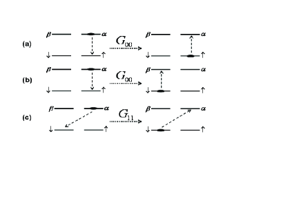
Figure 2: Illustration of a few possible photon exchanges between atoms when the interatomic separation is small. Owing to angular momentum conservation, only diagonal elements of $G$ are present. In (a) and (b) a transfer of excitation involving $\Delta m=0$ and, in (c), $\Delta m=1$, transitions is shown.

III.1 Coupled basis

As in lehmberg2 , the two-atom system can be described by superpositions of states that are either symmetrical or antisymmetrical under particle exchange (Dicke states). The indistinguishability of the particles restricts the system to the symmetric subspace. The ground state manifold is symmetrized as follows:

$$\left|g_{1~{}}\right\rangle \equiv\left|\uparrow\uparrow\right\rangle,$$ (13)

$$\left|g_{0}~{}\right\rangle \equiv\frac{1}{\sqrt{2}}\left(\left|\uparrow\downarrow\right\rangle+\left|\downarrow\uparrow\right\rangle\right),$$

$$\left|g_{-1~{}}\right\rangle \equiv\left|\downarrow\downarrow\right\rangle,$$

while ground-excited symmetric states are defined as:

$$\left|r_{1~{}}\right\rangle \equiv\frac{1}{\sqrt{2}}\left(\left|\alpha\uparrow\right\rangle+\left|\uparrow\alpha\right\rangle\right),$$ (14)

$$\left|r_{-1~{}}\right\rangle \equiv\frac{1}{\sqrt{2}}\left(\left|\beta\uparrow\right\rangle+\left|\uparrow\beta\right\rangle\right),$$

$$\left|s_{1~{}}\right\rangle \equiv\frac{1}{\sqrt{2}}\left(\left|\alpha\downarrow\right\rangle+\left|\downarrow\alpha\right\rangle\right),$$

$$\left|s_{-1~{}}\right\rangle \equiv\frac{1}{\sqrt{2}}\left(\left|\beta\downarrow\right\rangle+\left|\downarrow\beta\right\rangle\right).$$

Rewriting Eqs. (7) in terms of the new coefficients $r_{1,-1\text{~{}}}$and $s_{1,-1\text{~{}}}$, one finds

$$\overset{\cdot}{s}_{1~{}} =-\frac{5}{3}\gamma s_{1~{}}-i\Delta s_{1~{}}-\frac{1}{3}\gamma r_{-1~{}}+i\sqrt{2}\chi g_{-1~{}},$$ (15)

$$\overset{\cdot}{s}_{-1~{}} =-\frac{4}{3}\gamma s_{-1~{}}-i\Delta s_{-1~{}}{},$$

$$\overset{\cdot}{r}_{1~{}} =-\frac{4}{3}\gamma r_{1~{}}-i\Delta r_{1~{}}+i\chi g_{0~{}},$$

$$\overset{\cdot}{r}_{-1~{}} =-\frac{5}{3}\gamma r_{-1~{}}-i\Delta r_{-1~{}}-\frac{1}{3}\gamma s_{1~{}},$$

with quasistatic solutions

$$s_{1~{}} =\frac{i\sqrt{2}\chi\left(\frac{5}{3}\gamma+i\Delta\right)}{\left(\frac{5}{3}\gamma+i\Delta\right)^{2}-\frac{1}{9}\gamma^{2}}g_{-1~{}},$$ (16)

$$r_{1~{}} =\frac{i\chi}{i\Delta+\frac{4}{3}\gamma}g_{0~{}},$$

$$r_{-1~{}} =O\left[\left(\frac{\chi}{\Delta}\right)^{2}\right],$$

$$s_{-1~{}} =0.$$

Notice that the symmetric states containing the excited $\beta$ states have either identically zero or negligibly small amplitude, which substantially simplifies the calculation.

In the following two subsections, these expressions for the state amplitudes are used to derive the time evolution of the collective coherence and population. In the new basis the matrix elements are denoted by $\rho_{ij~{}}$, with $i,j=-1,0,1$.

III.1.1 Coherence decay

The expression for the collective coherence operator expectation value in the new basis is given by

$$\left\langle P_{\downarrow\uparrow~{}}\right\rangle=\sqrt{2}\left(\rho_{10~{}}+\rho_{0,-1~{}}\right).$$ (17)

In the limit $\gamma\ll\Delta$, the following rate equations are obtained for the out-terms [from Eq. (9)]

$$\overset{\cdot}{\rho}_{10~{}}^{out} =-\frac{4}{3}\gamma\frac{\chi^{2}}{\Delta^{2}}\rho_{10~{}},$$ (18)

$$\overset{\cdot}{\rho}_{0,-1}^{out} =-\frac{14}{3}\gamma\frac{\chi^{2}}{\Delta^{2}}\rho_{0,-1~{}},$$

while the in-terms, obtained from Eq. (10), evolve as

$$\overset{\cdot}{\rho}_{10~{}}^{in} =\frac{4}{3}\gamma\frac{\chi^{2}}{\Delta^{2}}\rho_{0,-1~{}},$$ (19)

$$\overset{\cdot}{\rho}_{0,-1~{}}^{in} =\frac{8}{3}\gamma\frac{\chi^{2}}{\Delta^{2}}\rho_{0,-1~{}}.$$

Adding the out-term contribution to the in-terms, and with the notation $\gamma_{op~{}}=\gamma\chi^{2}/\Delta^{2}$ (optical pumping rate), the equations for the density matrix elements relevant for the coherence decay are

$$\overset{\cdot}{\rho}_{10~{}} =-\frac{4}{3}\gamma_{op}\left(\rho_{10~{}}-\rho_{0,-1~{}}\right),$$ (20)

$$\overset{\cdot}{\rho}_{0,-1~{}} =-2\gamma_{op}\rho_{0,-1~{}}.$$

Substituting the solutions of the Eqs. (20) into Eq. (17), one obtains

$$\left\langle P_{\downarrow\uparrow~{}}(t)\right\rangle=\frac{1}{2}e^{-2\gamma_{op}t}\left(-1+3e^{\frac{2}{3}\gamma_{op}t}\right).$$ (21)

This is to be compared with the independent atom coherence decay derived in Appendix B [Eq. B4]

$$\left\langle P_{\downarrow\uparrow~{}}(t)\right\rangle^{ind}=e^{-\gamma_{op}t}.$$

Figure 3: Coupled system coherence decay for $R_{21}\ll\lambda$ vs. independent atoms decoherence.

The increase in the coherence decay rate for intermediate times, as shown in Fig. 3, can be understood in terms of the exchange processes in the uncoupled basis illustrated in Fig. 2. For an independent atom, the state $\left|\alpha\right\rangle$ is reached from the $\left|\downarrow\right\rangle$ state through the action of the classical field, and decays into $\left|\downarrow\right\rangle$ and $\left|\uparrow\right\rangle~{}$with rates $2(2\gamma/3)$ and $2(\gamma/3),$ respectively. In the cooperative case, other channels responsible for coherence generation or decay appear owing to the presence of the second atom.

An interesting behavior is observed at the initiation stage of the decoherence process, where the coupled system decoheres at a rate equal to that for independent atoms. However, this is not a general result, but rather a consequence of the initial state prepared with equal ground substate populations. When both atoms start in the same arbitrary state $a\left|\downarrow\right\rangle+b\left|\uparrow\right\rangle$ with $a\neq b$ and $a^{2}+b^{2}=1$, the evolution of the coupled system coherence takes the following form

$$\left\langle P_{\downarrow\uparrow~{}}(t)\right\rangle=2abe^{-2\gamma_{op}t}\left[-a^{2}+(1+a^{2})e^{\frac{2}{3}\gamma_{op}t}\right],$$ (22)

while the independent atom coherence evolves as:

$$\left\langle P_{\downarrow\uparrow~{}}(t)\right\rangle^{ind}=2abe^{-\gamma_{op}t}.$$ (23)

Expanding the exponentials in Eqs. (22) and (23) for small times $\gamma_{op}t\ll 1$, we find

$$\left\langle P_{\downarrow\uparrow~{}}(t)\right\rangle^{ind} \simeq 2ab\left(1-\gamma_{op}t\right),$$

$$\left\langle P_{\downarrow\uparrow~{}}(t)\right\rangle \simeq 2ab\left[1-\left(1+\frac{b^{2}-a^{2}}{3}\right)\gamma_{op}t\right]\text{,}$$ (24)

which shows that the decoherence rate of the coupled system is modified by the term $(b^{2}-a^{2})/3$. This indicates that, given a population imbalance between the up and down states, at the initiation stage, the decoherence rate of the coupled system can be either larger or smaller than the one for the independent atoms, and vanishes for the balanced case only, when $a=b=1/\sqrt{2}$.

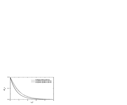
Figure 4: An ”imbalanced” superposition state with coefficients $a,b=1/10,\sqrt{99}/10$ decays exponentially at a rate $\gamma_{op}$, under the independent atoms assumption. However, when the decay is cooperative, an imbalanced state with $a<b$   decoheres at a faster rate than one with $a>b$.

III.1.2 Population Transfer

In the symmetric basis, the expectation value of the collective population operator is expressed as

$$\left\langle P_{\uparrow\uparrow~{}}\right\rangle=\rho_{11~{}}+\frac{1}{2}\rho_{00~{}}.$$ (25)

Three density matrix elements are coupled to each other: $\rho_{11~{}}$, $\rho_{00~{}}$and $\rho_{-1,-1~{}}$. The evolution resulting from the classical field can be obtained [from Eq. (9)] as

$$\overset{\cdot}{\rho}_{11~{}}^{out} =0,$$ (26)

$$\overset{\cdot}{\rho}_{00}^{out} =-\frac{8}{3}\gamma_{op}\rho_{00~{}},$$

$$\overset{\cdot}{\rho}_{-1,-1}^{out} =-\frac{20}{3}\gamma_{op}\rho_{-1,-1~{}},$$

while the in-terms are given by [see Eq. (10)]

$$\overset{\cdot}{\rho}_{11~{}}^{in} =\frac{4}{3}\gamma_{op}\rho_{00~{}},$$ (27)

$$\overset{\cdot}{\rho}_{00}^{in} =\frac{4}{3}\gamma_{op}\rho_{-1,-1~{}}+\frac{4}{3}\gamma_{op}\rho_{00~{}},$$

$$\overset{\cdot}{\rho}_{-1,-1}^{in} =\frac{16}{3}\gamma_{op}\rho_{-1,-1~{}}.$$

Combining the in-terms with out-terms, one finds rate equations

$$\overset{\cdot}{\rho}_{11~{}} =\frac{4}{3}\gamma_{op}\rho_{00~{}},$$ (28)

$$\overset{\cdot}{\rho}_{00} =\frac{4}{3}\gamma_{op}\left(\rho_{-1,-1~{}}-\rho_{00~{}}\right),$$

$$\overset{\cdot}{\rho}_{-1,-1} =-\frac{4}{3}\gamma_{op}\rho_{-1,-1~{}},$$

that are solved to give

$$\left\langle P_{\uparrow\uparrow~{}}(t)\right\rangle=1-\frac{1}{3}e^{-\frac{4}{3}\gamma_{op}t}\left(3+2\gamma_{op}t\right).$$ (29)

This is to be compared with the independent atom population evolution

$$\left\langle P_{\uparrow\uparrow~{}}(t)\right\rangle^{ind}=1-e^{-\frac{2}{3}\gamma_{op}t}.$$ (30)

where only one mechanism for populating state $\left|\uparrow\right\rangle$ is present: excitation of state $\left|\alpha\right\rangle$ by the classical field followed by decay at a rate $\gamma/3$ to state $\left|\uparrow\right\rangle$.

Figure 5: Cooperative optical pumping (from level $\left|\downarrow\right\rangle$ to level $\left|\uparrow\right\rangle$) for $R_{21}\ll\lambda$ vs. independent atoms optical pumping.

The increase in the population transfer rate, plotted in Fig. 5 vs. the independent atoms rate, is due to photons emitted by the second atom that drive the first atom into the $\left|\alpha\right\rangle$ state. A faster excitation of state $\left|\alpha\right\rangle~{}$leads to a faster transfer to $\left|\uparrow\right\rangle$ for intermediate times.

III.2 Mechanisms for coherence generation

It is interesting to isolate the dynamics of a single atom with the purpose of identifying the mechanisms that lead to the modification of its radiative properties due to the presence of a second atom in its vicinity. We analyze the rate of change of the expectation value of the one atom coherence operator $\sigma_{-~{}}^{(1)}=\left|\downarrow\right\rangle_{1}\left\langle\uparrow\right|_{1}$. This is expressed in terms of density matrix elements as $\left\langle\sigma_{-~{}}^{(1)}\right\rangle=\rho_{\uparrow\uparrow;\downarrow\uparrow~{}}+\rho_{\uparrow\downarrow;\downarrow\downarrow~{}}$, and it is found to satisfy the following equation of motion [using Eqs. (9) and (10)]

$$\frac{d}{dt}\left\langle\sigma_{-~{}}^{(1)}(t)\right\rangle=-\gamma_{op}\left\langle\sigma_{-~{}}^{(1)}(t)\right\rangle+\frac{1}{3}\gamma_{op}\left[\rho_{\downarrow\uparrow;\downarrow\downarrow~{}}-\rho_{\uparrow\uparrow;\uparrow\downarrow}\right].$$ (31)

The first term in the right-hand side in the above equation simply indicates the decay of the coherence of the independent atom at the expected rate $\gamma_{op}$. The second term contains the modification induced by the action of the neighboring atom. At the moment when the interaction between atoms is initiated, the density matrix of the coupled system can be factorized and this term can be written as: $-\frac{1}{3}\gamma_{op}\left\langle\sigma_{z~{}}^{(1)}\right\rangle\left\langle\sigma_{-~{}}^{(2)}\right\rangle$,  where $\sigma_{z~{}}^{(1)}=\left|\uparrow\right\rangle_{1}\left\langle\uparrow\right|_{1}-\left|\downarrow\right\rangle_{1}\left\langle\downarrow\right|_{1}$ is the population difference operator for the first atom. The significance of this term is that $x$ polarization (coherence) established in the second atom induces $x$ polarization in the first atom through the vacuum, given a population difference.

We proceed now to analyze the origin of this coupling term by considering two distinct situations in which atom $2$ is prepared in a superposition $a\left|\downarrow\right\rangle+b\left|\uparrow\right\rangle$ exhibiting coherence equal to $ab$, while atom $1$ is prepared either in the $\left|\uparrow\right\rangle$ state or the $\left|\downarrow\right\rangle$ state. In both cases no initial $x$ atomic polarization in the atom of interest is present. When starting with the population in the $\left|\uparrow\right\rangle$ state, using Eqs. (9) and (10), expressions for the density matrix elements present in the right-hand side of Eq. (31) can be derived, and an out-term is found to be responsible with the generation of coherence

$$\frac{d}{dt}\left\langle\sigma_{-~{}}^{(1)}(t)\right\rangle^{out} =-\frac{1}{3}\gamma_{op}ab,$$ (32)

$$\frac{d}{dt}\left\langle\sigma_{-~{}}^{(1)}(t)\right\rangle^{in} =0.$$

The process leading to this can be represented as follows

$$\rho_{\uparrow\uparrow;\uparrow\downarrow~{}}\overset{\chi}{\longrightarrow}\rho_{\uparrow\uparrow;\uparrow\alpha~{}}\overset{\gamma}{\longrightarrow}\rho_{\uparrow\uparrow;\alpha\uparrow~{}}\overset{\chi}{\longrightarrow}\rho_{\uparrow\uparrow;\downarrow\uparrow~{}},$$ (33)

where in the first step, the field induces an excitation in the second atom, followed by a swap of excitation between atoms through the vacuum (collision-like effect) and a stimulated emission from the first atom. In the second case, where the population is initially stored in the $\left|\downarrow\right\rangle$ state, both an in-term and an out-term are present:

$$\frac{d}{dt}\left\langle\sigma_{-~{}}^{(1)}(t)\right\rangle^{out} =-\frac{1}{3}\gamma_{op}ab,$$ (34)

$$\frac{d}{dt}\left\langle\sigma_{-~{}}^{(1)}(t)\right\rangle^{in} =\frac{2}{3}\gamma_{op}ab.$$

The coherence generation through the out-term is similar to the process shown above [Eq. (33)], while the in-term takes the following path

$$\rho_{\downarrow\uparrow;\downarrow\downarrow~{}}\overset{\chi}{\longrightarrow}\rho_{\downarrow\uparrow;\downarrow\alpha~{}}\overset{\chi}{\longrightarrow}\rho_{\alpha\uparrow;\downarrow\alpha~{}}\overset{\gamma}{\longrightarrow}\rho_{\uparrow\uparrow;\downarrow\uparrow~{}},$$ (35)

where consecutive excitations for both atoms are followed by spontaneous decay into a state with coherence in the first atom.

IV Arbitrary Separation

Simple analytical results are not available in this regime. Coupling through propagators other than $G_{ii~{}}$ takes place. The polarization of the emitted photon doesn’t have to match the one of the absorbed photon, a situation which is illustrated in Fig. 6, where the coupling of the two-atom state $\left|\alpha\uparrow\right\rangle$ to other states is shown and the corresponding elements of the $G$ matrix (including non-diagonal ones) responsible for the coupling specified.

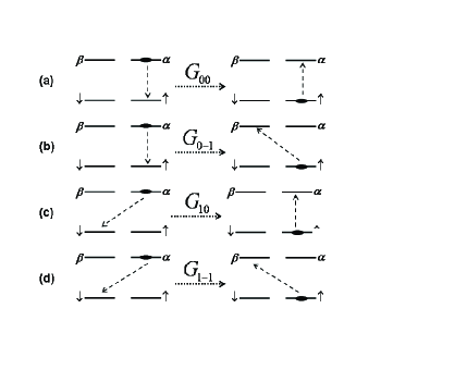
Figure 6: The transfer of excitation stored in the coupled state $\left|\alpha\uparrow\right\rangle~{}$can take place through a channel governed by a diagonal propagator $G_{00}$represented in (a), or through non-diagonal propagators $G_{01},$$G_{10}~{}$and $G_{1-1}~{}$as in (b), (c) and (d).

IV.1 Numerical Results

The calculations are now performed in the uncoupled basis. Numerical solutions of $12$ coupled rate equations give the coherence decay, whereas $13$ rate equations are solved to obtain the population transfer rate. The output of our numerical simulations is dependent both on time and on the spherical coordinates of the second atom $R_{21},\theta~{}$and $\varphi$. Since the system has azimuthal symmetry, the interesting cases are obtained by varying $R_{21}$ and $\theta$. Two orientations of the system with respect to the field propagation are examined: $\mathbf{R}_{21}~{}\|~{}$$\mathbf{k}_{L}~{}$($\theta=0$) and $\mathbf{R}_{21}~{}\bot~{}~{}$$\mathbf{k}_{L}~{}$($\theta=\pi/2$).

IV.1.1 Coherence Decay

The $4$ density matrix elements responsible for the coherence [Eq. (6)], are coupled to $8$ more through nondiagonal elements of $G$. A system of $12$ linear differential equations has to be solved containing $\left\{\rho_{\downarrow\downarrow;\downarrow\downarrow\text{ }},\rho_{\uparrow\downarrow;\downarrow\downarrow~{}},\rho_{\downarrow\uparrow;\downarrow\downarrow~{}},\rho_{\downarrow\downarrow;\uparrow\downarrow~{}},\rho_{\downarrow\downarrow;\downarrow\uparrow~{}},\rho_{\uparrow\uparrow;\downarrow\downarrow~{}},\rho_{\uparrow\downarrow;\uparrow\downarrow~{}},\rho_{\uparrow\downarrow;\downarrow\uparrow~{}},\rho_{\downarrow\uparrow;\downarrow\uparrow~{}},\rho_{\downarrow\uparrow;\uparrow\downarrow~{}},\rho_{\uparrow\uparrow;\uparrow\downarrow~{}},\rho_{\uparrow\uparrow;\downarrow\uparrow}\right\}$. The expressions for all $12$ rate equations are not given here; instead a single one is written to illustrate the way the coupling among different states comes into play

$$\overset{\cdot}{\rho}_{\uparrow\downarrow;\downarrow\downarrow~{}}=\frac{\gamma_{op}}{3}\left[\begin{array}[c]{c}-5\rho_{\uparrow\downarrow;\downarrow\downarrow~{}}-e^{-ik_{L}R_{21}\cos\theta}\left(\begin{array}[c]{c}\sqrt{2}G_{10~{}}(R_{21},\theta,\varphi)\rho_{\downarrow\downarrow;\downarrow\downarrow~{}}+2G_{00~{}}(R_{21},\theta,\varphi)\rho_{\downarrow\uparrow;\downarrow\downarrow~{}}\\ +2G_{11~{}}(R_{21},\theta,\varphi)\rho_{\uparrow\downarrow;\downarrow\downarrow~{}}\end{array}\right)\\ +e^{ik_{L}R_{21}\cos\theta}\left(\begin{array}[c]{c}2G_{11~{}}(R_{21},\theta,\varphi)\rho_{\uparrow\downarrow;\downarrow\downarrow~{}}+\sqrt{2}G_{01~{}}(R_{21},\theta,\varphi)\rho_{\uparrow\downarrow;\downarrow\uparrow~{}}\\ +\sqrt{2}G_{01~{}}(R_{21},\theta,\varphi)\rho_{\uparrow\downarrow;\uparrow\downarrow~{}}\end{array}\right)\end{array}\right].$$ (36)

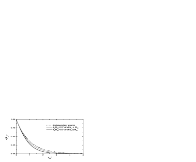
Figure 7: The two-atom coherence for $k_{L}R_{21}=0.7$ is plotted as a function of time for independent atoms, $\mathbf{R}_{21}~{}\|~{}$$\mathbf{k}_{L}~{}$and $\mathbf{R}_{21}~{}\bot~{}$$\mathbf{k}_{L}$, respectively. 

The time evolution of the collective coherence is shown in Fig. 7 for $k_{L}R_{21}=0.7$. For both $\mathbf{R}_{21}~{}\|~{}$$\mathbf{k}_{L}$ and $\mathbf{R}_{21}~{}\bot~{}$$\mathbf{k}_{L}$, the coherence decays more rapidly than for the independent atom case, and the decay for $\mathbf{R}_{21}~{}\|~{}$$\mathbf{k}_{L}$ is faster than that for $\mathbf{R}_{21}~{}\bot~{}$$\mathbf{k}_{L}$. To obtain some idea of the dependence of the decay rate on interatomic separation, we plot in Fig. 8 the decoherence rate ($\left\langle\overset{\cdot}{P}_{\uparrow\uparrow}(t)\right\rangle/\left\langle P_{\uparrow\uparrow}(t)\right\rangle$) as a function of distance, at a fixed time $t=1/\gamma_{op}$, for both the $\mathbf{R}_{21}~{}\|~{}\mathbf{k}_{L}~{}$and $\mathbf{R}_{21~{}}\bot~{}\mathbf{k}_{L}$. Even though a numerical solution has been used to obtain the plot in Fig. 8, an approximate analytical treatment can provide insight into the qualitative nature of the results. In particular it can help explain why the parallel case decay rate is larger than that for closely separated atoms. The coupled equations of motion for the coherence operators associated with each atom [similar to Eq. (31) but with the difference that now the coupling coefficients are $R_{21}~{}$dependent] are solved approximately at a fixed time.

It is found that the perpendicular case differs from the close atoms case only insofar as the coupling between atoms is modulated by the real part of $G_{00~{}}(R_{21~{}},\pi/2,0)$. An analytical expression for a fixed time $t=1/\gamma_{op}$ gives a decoherence rate of the collective coherence that varies with the separation as $\gamma_{op}[1+0.21\operatorname{Re}(G_{00~{}}(R_{21},\pi/2,0))]$.

There is, however, a fundamental difference between the perpendicular and parallel case that is reflected in the system’s response. In the perpendicular case the spatial phase of the laser field does not enter since $\mathbf{k}_{L}\cdot\mathbf{R}_{21}=0$. As a result the spin coherence associated with each atom evolves in an identical fashion. On the other hand, in the parallel case there is a relative phase difference of $\mathbf{k}_{L}\cdot\mathbf{R}_{21}$ associated with the laser field as it interacts with atoms at the two sites. Consequently, the response of the two atoms need no longer be identical, since the spatial symmetry has been broken by the field. Three coupling terms are present in the parallel case: $\operatorname{Re}(G_{00~{}}(R_{21},0,0)\cos k_{L}R_{21})$, $\operatorname{Re}(G_{00~{}}(R_{21},0,0)\sin k_{L}R_{21})~{}$and $\operatorname{Re}(G_{11~{}}(R_{21},0,0)\sin k_{L}R_{21})$; the importance of the laser induced spatial phase is evident in these expressions. Owing to the extra couplings, the two atoms accumulate different spatial phases, and the collective coherence (obtained as the sum of individual coherences) shows a spatial modulation that varies as $\operatorname{Re}(G_{11~{}}(R_{21},0,0)\sin k_{L}R_{21})$. A full analytical solution for the variation of the decay rate with the distance for any fixed time is not available; however, a perturbative treatment for small times ($\gamma_{op}t\ll 1$) indicates an increase in the decay rate $2/9$ $\operatorname{Re}(G_{11~{}}^{2}(R_{21},0,0)\sin^{2}k_{L}R_{21})\gamma_{op}^{2}t$.

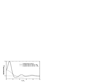
Figure 8: For a fixed time $t=1/\gamma_{op}$, the decoherence rate of the two atoms (in units of $\gamma_{op}$) is plotted for separations varying from $0~{}$to $R_{21}=10/k_{L}$. The dotted line respresents the independent atom decoherence rate ($\gamma_{op}$).

Just as in the case of close atoms, we extend our simulations to analyze the decay of an arbitrary initial state $a\left|\downarrow\right\rangle+b\left|\uparrow\right\rangle$. The observed behavior is quite different here. Even for relatively large separation ($R_{21}=\lambda/2\pi$), a state with most population in the down state decays much faster than in the independent atom case, while an inhibition of decoherence is obtained when the initial state is prepared with more population in the up state [as shown in Fig. 9 for $\mathbf{R}_{21}~{}\|~{}$$\mathbf{k}_{L}$ and $\mathbf{R}_{21}~{}\bot~{}$$\mathbf{k}_{L}$].

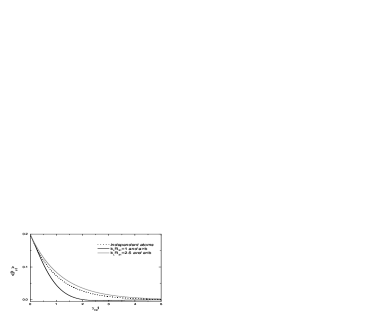
Figure 9: The decay of the collective coherence of an ”imbalanced” superposition state with coefficients $1/10~{}$and $\sqrt{99}/10$ is plotted above. Enhancement of the decay rate can be obtained when the initial state has more population in the up state, while the opposite case gives rise to an inhibition of decoherence.

IV.1.2 Optical Pumping

One more density matrix element ($\rho_{\uparrow\uparrow;\uparrow\uparrow~{}}$) is coupled to the $12$ listed before and a system of $13$ rate equations is solved to obtain the collective population transfer as a function of time.

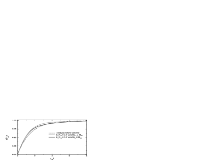
Figure 10: The population transfer for $k_{L}R_{21}=0.7$ is plotted for independent atoms, $\mathbf{R}_{21}~{}\|~{}$$\mathbf{k}_{L}~{}$and $\mathbf{R}_{21}~{}\bot~{}$$\mathbf{k}_{L}$, respectively. 

An interesting behavior is obtained in both the parallel and perpendicular cases (see Fig. 10): the optical pumping rate is initially larger and afterwards smaller than the one for independent atoms. The saturation effect at large times is due to the addition of a decay channel (the $\left|\beta\right\rangle~{}$state) which provides a way for the transfer of population from $\left|\uparrow\right\rangle$ back to the initial $\left|\downarrow\right\rangle$ state. This accounts for a slow down at large times where the repopulation from the second atom (resulting in population in state $\left|\beta\right\rangle$) is comparable with the population produced by the classical field.

V Polarization swap

As seen in Sec. III B, a partial transfer of coherence from an $x~{}$polarized atom to an initially unpolarized atom (in a $z$ state, either up or down) can be achieved. The two distinct situations discussed there can be extended for variable interatomic separations. Figures 11 and 12 show the evolution of the coherence of the first atom as a function of time for $R_{21}\ll\lambda$ and $R_{21}=\lambda/2\pi$ and $\lambda/\pi$, respectively, when $\mathbf{R}_{21}~{}\|~{}$$\mathbf{k}_{L}$. In both cases, owing to the oscillating nature of the coupling between atoms (as a function of separation) the sign of the effect produced in the initially $z$ polarized atom depends dramatically on the distance.

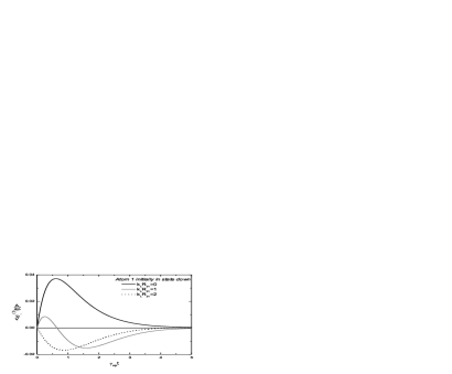
Figure 11: An $x~{}$polarized atom $2~{}$induces an $x~{}$polarization in an initially $z~{}$polarized atom $1~{}$(spin down). The coherence in atom $1~{}$is plotted as a function of time at $R_{21}\ll\lambda$, at $R_{21}=1/k_{L}~{}$and at $R_{21}=2/k_{L}$, for the case when $\mathbf{R}_{21}~{}\|~{}$$\mathbf{k}_{L}$.

The decay dynamics are still given by Eqs. (32) and (34), with the distinction that the decay parameter, which for close atoms is simply equal to $\gamma_{op}/3$, is now spatially modulated by $G_{00}(R_{21},0,0)\cos(k_{L}R_{21})$. In the case where the first atom is initially in the up state, the coherence is driven only by the out-term, which leads to a simple time behavior, where $\left\langle P_{\uparrow\uparrow}(t)\right\rangle$ changes sign only due to the spatial oscillation of the coupling term. In contrast, in the down case, the competition between the in-term and out-term leads to a change in the sign of $\left\langle P_{\uparrow\uparrow}(t)\right\rangle$ for intermediate distances.

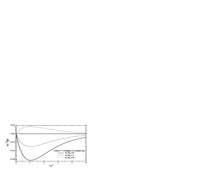
Figure 12: Atom $1$ starts here in state up. The polarization transfer is plotted as a function of time at $R_{21}\ll\lambda$, at $R_{21}=1/k_{L}~{}$and $R_{21}=2/k_{L}$, for the case when $\mathbf{R}_{21}~{}\|~{}$$\mathbf{k}_{L}$.

VI Conclusions

We examined a system of two multilevel atoms coherently driven by a single-mode classical laser field and coupled to the electromagnetic vacuum. The decoherence (of a quantum superposition stored in the ground sublevels) that necessarily accompanies the process of manipulation of the atomic states has been analyzed in the context of cooperative behavior. Two cases have been treated, where the atoms are either at the same position or separated by a distance comparable to the optical wavelength. It has been found (not surprisingly) that, for the case of close atoms, the ”communication” between atoms leads to an increase in both the decoherence and population transfer rates. With increasing interatomic separation, in the case of the field propagating perpendicularly to the line joining the atoms, the decoherence rate is less than that for close atoms. This is an expected result since, from the point of view of the classical field the atoms are located at equivalent positions, and a simple decrease of the interatomic coupling due to the increasing separation is expected. For certain distances, however, owing to the oscillating behavior of this coupling, a small effect of decoherence inhibition is also observed. A more interesting situation arises for the case when the atoms are aligned parallel to the field propagation direction. The equivalency of positions does not hold here anymore, and a spatial phase difference between atoms resulting from the classical field is established. The coupling through the vacuum is modulated by this spatial phase difference, and a considerable enhancement in the decay rate is observed at separations of order $\lambda/2\pi$. These results will be generalized in a future planned publication to a large ensemble of atoms in a pencil-shaped geometry. In such a medium, at Fresnel numbers close to unity, the atoms are practically aligned along the direction of the field; for large optical depths, the phase effect described above is expected to lead to a substantial increase in the decay of the collective atomic coherence.

VII Acknowledgments

This work is supported by the National Science Foundation under Grant No. PHY-0244841 and the FOCUS Center grant.

VIII Appendix A: Explicit expressions for propagators

The expressions for the propagators involve spherical harmonics and Hankel functions of the first kind, $h_{0}(k_{0}R)$ and $h_{2}(k_{0}R)$ [Ref. hao-berman ]:

$$G_{11}(\mathbf{R}) =\sqrt{4\pi}h_{0}(k_{0}R)Y_{0,0}(\widehat{\mathbf{R}})-\frac{1}{2}\sqrt{\frac{4\pi}{5}}h_{2}(k_{0}R)Y_{2,0}(\widehat{\mathbf{R}}),$$ (A1)

$$G_{00}(\mathbf{R}) =\sqrt{4\pi}h_{0}(k_{0}R)Y_{0,0}(\widehat{\mathbf{R}})+\sqrt{\frac{4\pi}{5}}h_{2}(k_{0}R)Y_{2,0}(\widehat{\mathbf{R}}),$$

$$G_{1,-1}(\mathbf{R}) =-\frac{3}{2}\sqrt{\frac{8\pi}{15}}h_{2}(k_{0}R)Y_{2,-2}(\widehat{\mathbf{R}}),$$

$$G_{-1,1}(\mathbf{R}) =-\frac{3}{2}\sqrt{\frac{8\pi}{15}}h_{2}(k_{0}R)Y_{2,2}(\widehat{\mathbf{R}}),$$

$$G_{1,0}(\mathbf{R}) =-\frac{3}{2}\sqrt{\frac{4\pi}{15}}h_{2}(k_{0}R)Y_{2,-1}(\widehat{\mathbf{R}}),$$

$$G_{-1,0}(\mathbf{R}) =-\frac{3}{2}\sqrt{\frac{4\pi}{15}}h_{2}(k_{0}R)Y_{2,1}(\widehat{\mathbf{R}}),$$

$$G_{-1,-1}(\mathbf{R}) =G_{1,1}(\mathbf{R});\text{ \ }G_{0,-1}(\mathbf{R})=-G_{1,0}(\mathbf{R});\text{ \ }G_{0,1}(\mathbf{R})=-G_{-1,0}(\mathbf{R}).$$

IX Appendix B: Derivation of the decoherence and population transfer rates for a single 4-level atom

We explicitly derive the equations of motion for the ground state coherence and populations for a single 4-level atom interacting with a $\sigma_{+}$ polarized field. In the perturbative limit where a maximum of one excitation is allowed, a basis set in the Hilbert space of atom and radiation field is comprised of states $\left|\downarrow\right\rangle\left|0\right\rangle$, $\left|\uparrow\right\rangle\left|0\right\rangle\,$, $\left|\alpha\right\rangle\left|0\right\rangle$, $\left|\beta\right\rangle\left|0\right\rangle$, $\left|\downarrow\right\rangle\left|\mathbf{k},\lambda\right\rangle$ and $\left|\uparrow\right\rangle\left|\mathbf{k},\lambda\right\rangle$. The first ket denotes the state of the atom while, the second one describes a vacuum field or a one photon state with wave number $\mathbf{k}$ and polarization $\lambda$. The state amplitudes obey the following equations of motion:

$$\overset{\cdot}{b}_{\alpha;0~{}} =-\gamma b_{\alpha;0~{}}-i\Delta b_{\alpha;0~{}}+i\chi b_{\downarrow 0~{}},$$ (B1)

$$\overset{\cdot}{b}_{\beta;0~{}} =-\gamma b_{\beta;0~{}}-i\Delta b_{\beta;0~{}},$$

$$\overset{\cdot}{b}_{\downarrow;0~{}} =i\chi b_{\alpha;0~{}},$$

$$\overset{\cdot}{b}_{\uparrow;0~{}} =0,$$

$$\overset{\cdot}{b}_{\downarrow;\mathbf{k},\lambda~{}} =ig_{\mathbf{k},\lambda~{}}^{\downarrow\alpha}b_{\alpha;0~{}},$$

$$\overset{\cdot}{b}_{\uparrow;\mathbf{k},\lambda~{}} =ig_{\mathbf{k},\lambda~{}}^{\uparrow\beta}b_{\beta;0~{}}.$$

Using a master equation approach one can write density matrix equations of motion for the ground state sublevels as:

$$\overset{\cdot}{\rho}_{\uparrow\uparrow~{}} =2\left(\frac{2\gamma}{3}\right)\rho_{\beta\beta~{}}+2\left(\frac{\gamma}{3}\right)\rho_{\alpha\alpha~{}},$$ (B2)

$$\overset{\cdot}{\rho}_{\downarrow\uparrow~{}} =-2\left(\frac{2\gamma}{3}\right)\rho_{\alpha\beta~{}}+i\chi\rho_{\alpha\uparrow~{}},$$

$$\overset{\cdot}{\rho}_{\downarrow\downarrow~{}} =2\left(\frac{\gamma}{3}\right)\rho_{\beta\beta~{}}+2\left(\frac{2\gamma}{3}\right)\rho_{\alpha\alpha~{}}+i\chi\left(\rho_{\downarrow\alpha}-\rho_{\alpha\downarrow}\right).$$

The first observation that we make here is that the terms in the right hand side of the above equations, that are due to the field (out-terms) and to the coupling to the vacuum (in-terms) can be derived separately. In other words, the presence of dissipation can be neglected when writing equations describing the driving effect of the field and later added to the equations phenomenologically. The derivation of rate equations can now be carried out by writing equations for the ground-excited coherences and excited state populations and coherences and adiabatically eliminating them. However, this is an unnecessary complication; the second observation that we make provides an easier way of doing this. Only the first $4$ equations in Eqs. (B1) have to be solved and the excited amplitudes can be written in terms of ground state amplitudes. Next, the density matrix elements can be written simply as if the state of the system were a pure state (as products of amplitudes) and replaced in Eqs. (2) to obtain rate equations. The separation of in-terms from out-terms in these equations insures the validity of this approach. Following this recipe, it is found that (in the limit $\Delta\gg\gamma$)

$$\rho_{\alpha\beta~{}} =b_{\alpha;0~{}}b_{\beta;0~{}}^{\ast}=0,$$ (B3)

$$\rho_{\alpha\alpha~{}} =b_{\alpha;0~{}}b_{\alpha;0~{}}^{\ast}\simeq\frac{\chi^{2}}{\Delta^{2}}b_{\downarrow 0~{}}b_{\downarrow 0~{}}^{\ast}=\frac{\chi^{2}}{\Delta^{2}}\rho_{\downarrow\downarrow~{}},$$

$$\rho_{\beta\beta~{}} =b_{\beta;0~{}}b_{\beta;0~{}}^{\ast}=0,$$

$$\rho_{\alpha\uparrow~{}} =b_{\alpha;0~{}}b_{\uparrow;0~{}}^{\ast}\simeq i\gamma\frac{\chi}{\Delta^{2}}b_{\downarrow 0~{}}b_{\uparrow 0~{}}^{\ast}+\frac{\chi}{\Delta}b_{\downarrow 0~{}}b_{\uparrow 0~{}}^{\ast}=i\gamma\frac{\chi}{\Delta^{2}}\rho_{\downarrow\uparrow~{}}+\frac{\chi}{\Delta}\rho_{\downarrow\uparrow~{}},$$

$$\rho_{\downarrow\alpha~{}} =b_{\downarrow;0~{}}b_{\alpha;0~{}}^{\ast}=i\gamma\frac{\chi}{\Delta^{2}}b_{\downarrow 0~{}}b_{\downarrow 0~{}}^{\ast}+\frac{\chi}{\Delta}b_{\downarrow 0~{}}b_{\downarrow 0~{}}^{\ast}=i\gamma\frac{\chi}{\Delta^{2}}\rho_{\downarrow\downarrow~{}}+\frac{\chi}{\Delta}\rho_{\downarrow\downarrow~{}},$$

$$\rho_{\alpha\downarrow~{}} =\rho_{\downarrow\alpha~{}}^{\ast}.$$

Replacing these expressions into Eqs. (B2), rate equations are obtained in a final form:

$$\overset{\cdot}{\rho}_{\uparrow\uparrow~{}} =\frac{2}{3}\gamma_{op}\rho_{\downarrow\downarrow~{}},$$ (B4)

$$\overset{\cdot}{\rho}_{\downarrow\uparrow~{}} =-\gamma_{op}\rho_{\downarrow\uparrow~{}}+i\frac{\chi^{2}}{\Delta}\rho_{\downarrow\uparrow~{}},$$

$$\overset{\cdot}{\rho}_{\downarrow\downarrow~{}} =\frac{4}{3}\gamma_{op}\rho_{\downarrow\downarrow~{}}-2\gamma_{op}\rho_{\downarrow\downarrow~{}}=-\frac{2}{3}\gamma_{op}\rho_{\downarrow\downarrow~{}}.$$

The decoherence of an initial state $\frac{1}{\sqrt{2}}\left(\left|\downarrow\right\rangle+\left|\uparrow\right\rangle\right)$ can now be calculated as described by the evolution of $\rho_{\downarrow\uparrow~{}}$(neglecting the phase associated with the AC Stark shift)

$$\rho_{\downarrow\uparrow~{}}(t)=\frac{1}{2}e^{-\gamma_{op}t},$$ (B5)

while the population transfer from state $\left|\downarrow\right\rangle$ to state $\left|\uparrow\right\rangle$ is given by

$$\rho_{\uparrow\uparrow~{}}(t)=1-e^{-\frac{2}{3}\gamma_{op}t}.$$ (B6)

References

- (1) R. H. Dicke, Phys. Rev. 93, 99 (1954).
- (2) V. Ernst and P. Stehle, Phys. Rev. 176, 1456 (1968).
- (3) R. H. Lehmberg, Phys. Rev. A 2, 883 (1970).
- (4) G. S. Agarwal, Phys. Rev. A 2, 2038 (1970).
- (5) J. H. Eberly, Am. J. Phys. 40, 1374 (1972).
- (6) D. F. Walls, J. Phys. B 13, 2001 (1980).
- (7) R. H. Lehmberg, Phys. Rev. A 2, 889 (1970).
- (8) Z. Ficek, R. Tanaś and S. Kielich, Optics Comm. 36, 121 (1981).
- (9) Th. Richter, Optica Acta 30, 1769 (1983).
- (10) L.-M. Duan, J. I. Cirac, P. Zoller and E. S. Polzik, Phys. Rev. Lett. 85, 5643 (2000); L.-M. Duan and H. J. Kimble, Phys. Rev. Lett. 90, 253601 (2003).
- (11) L. K. Thomsen, S. Mancini and H. M. Wiseman, Phys. Rev A 65, 061801 (2002); S. Massar and E. S. Polzik, Phys. Rev. Lett. 91, 060401 (2003); J. K. Stockton, R. van Handel and H. Mabuchi, Phys. Rev. A 70, 022106 (2004); C. Genes and P. R. Berman, Phys. Rev. A 73, 013801 (2006).
- (12) R. Bonifacio, P. Schwendimann and F. Haake , Phys. Rev A 4, 302 (1971); D. Polder, M. F. H. Schuurmans and Q. H. F. Vrehen, Phys. Rev A 19, 1192 (1979).
- (13) It should be noted that the qualitative results for this particular case cannot be generalized to other level scheme or field polarization. For example, a calculation on two close atoms (not presented here) that uses instead of polarized driving fields and the same transition, indicates that the collective decoherence rate is not different from the independent atom coherence decay rate.
- (14) Hao Fu and P. R. Berman, Phys. Rev. A 72, 022104 (2005).
- (15) P. R. Berman and P.W. Milonni, Phys. Rev. Lett. 92, 053601 (2004).
- (16) B. Dubetsky and P. R. Berman, Phys. Rev A 53, 390 (1996).