Generalized Bloch Spheres for m-Qubit States.

Abstract

m-Qubit states are embedded in $\mathfrak{Cl}_{2m}$ Clifford algebra. Their probability spectrum then depends on $O\left(2m\right)$- or $O\left(2m+1\right)$-invariants respectively. Parameter domains for $O\left(2m\left(+1\right)\right)$-vector and -tensor configurations, generalizing the notion of a Bloch sphere, are derived.

1 Introduction

For many purposes it is useful to consider m-qubit states as vectors in a $\mathbb{R}$-linear Hilbert space $\mathfrak{H}$ whose basis is a set $\{B_{i},\;i=1\ldots 2^{2m}\}$ of $2^{m}\times 2^{m}$ orthonormal

$$\text{trace}\left(B_{i}\cdot B_{j}\right)=\delta_{ij},$$

hermitian matrices:

$$\mathfrak{H}=\{\sum_{k=1}^{2^{2m}}b_{k}\;B_{k}\;|\;b_{k}\;\;\text{real}\}.\qquad\left(H\right)$$

A state is either represented by a hermitian, normalized matrix or an appropriate coordinate vector $\left[b_{1},b_{2},\ldots,b_{2^{2m}}\right]$ (a formulation in an appropriate projective space would more adequate).In [2] [3] the generators of the quantum invariance group $SU\left(2^{m}\right)$ are proposed as such a basis, a possibility which we shall discuss in the Summary.
A straightforward solution for the parametrisation of a state $\varrho$ (a density matrix) is to write the set of all states as

$$\{\varrho\}=\bigcup_{\Lambda}\rho_{\Lambda}^{\mathfrak{U}}$$

where

$$\rho_{\Lambda}^{\mathfrak{U}}=\{U^{+}\varrho_{\Lambda}U\;|\;U\in\mathfrak{U}\left(2^{m}\right)\}$$

and

$$\text{$\varrho_{\Lambda}$ is the diagonal matrix}\;\;\varrho_{\Lambda}=\text{diag}\{\Lambda\},$$

$$\Lambda=\{[\lambda_{1},\lambda_{2},\ldots,\lambda_{2^{m}}]\;|\;\lambda_{i}\text{ real, }\sum\lambda_{i}=1,\;\lambda_{i}\geq 0\};$$

$\mathfrak{U}\left(2^{m}\right)$ is the unitary group in $2^{m}$-dimensions and $\Lambda$ is the probability spectrum generating the State $\rho_{\Lambda}^{\mathfrak{U}}$. This construction warrants positivity and normalisation. It is however not always (or, better, almost never) convenient in the discussion of physical situations. On the other hand writing $\varrho$ as a vector in $\mathfrak{H}$ confronts us with the problem of deriving conditions for the expansion coefficients that guarantee the expansion to yield a state. Formulated in this general way the problem has no obvious solution: positivity and normalisation conditions can derived by expressing the eigenvalues in terms of the expansion coefficients, i.e. finding the zeroes of the characteristic polynomial as functions of these parameters. As we know from Abel and Galois a solution by rational operations and radicals does not exist for quintic or higher degrees, i.e. for general 3-qubit and a fortiori for higher systems. For the 2-qubit explicit expressions are given by the Ferrari-Cardano formulae.
In this paper I explicitly construct classes of states for all $m$ whose spectra are determined by charactistic polynomials factorizing into polynomials of a given degree. The novel point in our considerations is the use of hermitian matrix representations of a Clifford algebra to construct bases in $\mathfrak{H}$. This particular choice of basis allows us to arrange the $2^{2m}-1$ real coordinates of a m-Qubit state in multidimensional arrays which are shown to ’transform’ as $O\left(2m\right)$ tensors. This fact implies that the probability spectrum of a m-Qubit state depends only on $O\left(2m\right)$-invariants, a considerable simplification of the parameter dependencies of these eigenvalues, indeed. This simplification leads to a complete characterisation of complete sets of states which allow for an explicit construction of a parameter domain. In this way I find the set of all states (vector-states) whose parameter domain is the Bloch $2m$-sphere. Furthermore a set of (bivector)-states is proposed whose novel parameter domain generalizes the notion of a Bloch sphere. Beyond these two domains the Descartes rule for the positivity of polynomial roots can be used to derive admissible parameter domains.

2 m-Qubit states imbedded in Clifford Algebras.

An m-qubit system is controlled by $m$ spin-degrees of freedom and hence by $2^{2m}-1$ parameters (see footnote 2 on page 2). The determining anticommutation relation for Clifford numbers [1] ($\mathbb{I}$ is the unity)

$$\Gamma_{i}\cdot\Gamma_{j}\;+\;\Gamma_{j}\cdot\Gamma_{i}=2\delta_{ij}\;\mathbb{I}$$ (1)

with

$$i,j=1\ldots 2m$$

has $2^{m}$-dimensional, hermitian, traceless matrix representations $\Gamma^{\{m\}}_{j}$.
From the anticommutation relations we see immediately that the products

$$\Gamma_{j_{1},j_{2},\ldots,j_{k}}:=i^{k-1}\;\Gamma_{j_{1}}\cdot\Gamma_{j_{2}}\cdot\;\ldots\;\cdot\Gamma_{j_{k}}$$ (2)

$$k=2\ldots m$$ (3)

are totally anti-symmetric in the indices $\left[j_{1}\ldots j_{k}\right]$. The only symmetric object constructed from Clifford numbers is the unity

$$\mathbb{I}=\Gamma_{i}^{2}$$

as we see from the anticommutation relations. A product consists of at most $2m$ factors. Hence we have

$$\sum_{k=0}^{2m}\binom{2m}{k}=2^{2m}$$

independent products. Furthermore because of the commutation relations we have

$$\text{trace}\left(\left(\Gamma^{\{m\}}_{i_{1}}\cdot\Gamma^{\{m\}}_{j_{1}}\cdot\;\ldots\;\cdot\Gamma^{\{m\}}_{k_{1}}\right)^{+}\Gamma^{\{m\}}_{i_{2}}\cdot\Gamma^{\{m\}}_{j_{2}}\cdot\;\ldots\;\cdot\Gamma^{\{m\}}_{k_{2}}\right)\sim$$

$$\sum\left(\delta_{\bar{i}_{1}\bar{i}_{2}}\delta_{\bar{j}_{1}\bar{j}_{2}}\ldots\delta_{\bar{k}_{1}\bar{k}_{2}}\right),$$

$$\text{where the $\delta$-function expresses pairwise equality of the $\cdot_{1}$- and $\cdot_{2}$-indices}.$$

A hermitian $2^{m}\times 2^{m}$-matrix requires $2^{2m}$ real numbers for a complete para-metrisation. Thus m-qubit states can be expanded in terms of $\mathbb{I}$ and the products introduced: Clifford numbers are the starting point for the construction of a basis in the $\mathbb{R}$-linear space of hermitian matrices:
this basis is construed as a Clifford algebra $\mathfrak{Cl}_{2m}$ ($2^{2m}$-dimensional as we have seen). The important advantage to gain from this choice of basis is that now domains for parameters are determined by $O\left(2m\right)$-invariants. The number of parameters necessary for the specification of these domains is thus considerably reduced. For the domains found in this paper this means one invariant for the vector-state configuration ($2m$ parameters) and two invariants for the bivector states ($m\left(2m-1\right)$ parameters) to be constructed below for all $m$.
I should remark that many beautiful geometric reverberations of Clifford algebras will play no rôle here, only very elementary properties of Clifford algebras will be sketched, emphasizing practical aspects. It is in this sense that the following, hopefully selfcontained, outline of the method should be understood.
To construct a basis and its matrix representation $\mathfrak{G}^{\{m\}}$ in $\mathfrak{H}$
I proceed as follows:

• The product

  $$\Gamma^{\{m\}}_{2m+1}:=\left(-i\right)^{m}\;\;\Gamma^{\{m\}}_{1}.\Gamma^{\{m\}}_{2}.\ldots\Gamma^{\{m\}}_{2m}$$ (4)

  obviously anti-commutes with all the $\Gamma^{\{m\}}_{i}\;\,i=1\ldots 2m$.

• The explicitly anti-symmetric products ($\varepsilon$ is the totally anti-symmetric symbol in $2m$-dimensions)

  $$\hat{\Gamma}^{\{m,k\}}_{i_{1}\ldots i_{k}}=F_{Norm}^{\{m,k\}}\;\left(\varepsilon_{i_{1}\ldots i_{2m}}\;\Gamma^{\{m\}}_{i_{k+1}}.\ldots\Gamma^{\{m\}}_{2m}\right)\Gamma^{\{m\}}_{2m+1}$$ (5)

  $$F_{Norm}^{\{m,k\}}=\frac{\left(-i\right)^{m+s}}{\left(2m\right)!}\binom{2m}{k}$$

  $$s=\begin{cases}0\;\,&\text{when }\;x=0,1\\ 1\;\,&\text{when }\;x=2,3\end{cases}\quad\text{where }\;\,x=k\,mod\left(4\right)$$ (6)

  The limiting cases $k=1$ and $k=2m$ are immediately seen to be

  $$\hat{\Gamma}^{\{m,1\}}_{i_{1}}\;=\;\left(-1\right)^{m+1}\Gamma^{\{m\}}_{i_{1}}$$

  $$\hat{\Gamma}^{\{m,2m\}}_{i_{1}\ldots i_{2m}}=\frac{f_{m}}{2m!}\;\varepsilon_{i_{1}\ldots i_{2m}}\;\Gamma^{\{m\}}_{2m+1}$$

  with

  $$f_{m}=\begin{cases}\left(-1\right)^{\frac{m}{2}}&\quad\text{for m even}\\ \left(-1\right)^{\frac{m+1}{2}}&\quad\text{for m odd}\end{cases}$$

• Because of the anti-commutation relations the only symmetric tensor is the scalar, i.e. the unit matrix

  $$\hat{\Gamma}^{\{m,0\}}\;=\;\mathbb{I}$$ (7)

• The set of matrices ${\mathfrak{G}}^{\{m\}}\;=\;\{\hat{\Gamma}^{\{m,0\}},\hat{\Gamma}^{\{m,1\}}\;\;\ldots\;\;\hat{\Gamma}^{\{m,2m\}}\}$ is orthonormal in the sense of (1).

• Formally speaking this gives an identification of the linear spaces
  $\mathfrak{g}^{\{m,k\}}=\text{span}\left(\hat{\Gamma}^{\{m,k\}},\mathbb{R}\right)$ and the tensor algebra $\overset{k}{\bigwedge}\;\mathbb{R}^{2m}$ of $\mathbb{R}^{2m}$. In detail we write

  Isomorphic vector spaces:

  $$\text{scalar},\;\,\mathbb{R}\qquad |\qquad\mathfrak{g}^{\{m,0\}}=\mathbb{R}\cdot\mathbb{I}$$

  $$\text{vector},\;\,\overset{1}{\bigwedge}\;\mathbb{R}^{2m}=\mathbb{R}^{2m}\qquad |\qquad\hat{\mathfrak{g}}^{\{m,1\}}$$

  $$\text{(2-)tensor (bivector)},\;\,\overset{2}{\bigwedge}\;\mathbb{R}^{2m}\qquad |\qquad\hat{\mathfrak{g}}^{\{m,2\}}$$

  $$\ldots \ldots$$

  $$\text{volume element},\;\,\overset{2m}{\bigwedge}\;\mathbb{R}^{2m}\qquad |\qquad\hat{\mathfrak{g}}^{\{m,2m\}}$$

• Following these observations we organize the state-parameters in terms of a scalar $G_{0}^{\{m,0\}}$ and the totally anti-symmetric real arrays

  $$G_{i_{1}}^{\{m,1\}},\;G_{i_{1},i_{2}}^{\{m,2\}}\;\ldots\;G_{i_{1},i_{2},\ldots,i_{2m}}^{\{m,2m\}}$$

  (i.e. totally antisymmetric arrays of real numbers)

  and thus account for

  $$\sum_{k=0}^{2m}\binom{2m}{k}\;=\;2^{2m}$$ (8)

  coefficients.

• We write the expansion of a m-qubit state as

  $$\varrho^{\{m\}}\;=\;\sum_{k=0}^{2m}G^{\{m,k\}}\circ\hat{\Gamma}^{\{m,k\}}$$ (9)

  where $\circ$ indicates the contraction $A\circ B=\sum_{i_{1},\ldots,i_{k}}A_{i_{1},\ldots,i_{k}}B_{i_{1},\ldots,i_{k}}$.

• An explicit construction of the representation $\Gamma^{\{m\}}_{1},\ldots,\Gamma^{\{m\}}_{2m}$ traditionally proceeds e.g. as follows:
  Starting with the Pauli matrices

  $$\sigma_{1}=\begin{pmatrix}0&1\\ 1&0\end{pmatrix},\quad\sigma_{2}=\begin{pmatrix}0&-I\\ I&0\end{pmatrix},\quad\sigma_{3}=\begin{pmatrix}1&0\\ 0&-1\end{pmatrix},\quad\sigma_{4}=\begin{pmatrix}1&0\\ 0&1\end{pmatrix},\quad$$

  we have the iteration scheme

  $${\mathfrak{G}}^{\{m+1\}}\;=$$

  $$\{\Gamma^{\{m,1\}}\times\sigma_{1},\ldots,\Gamma^{\{m,2m\}}\times\sigma_{1},\Gamma^{\{m,0\}}\times\sigma_{2},\;\,\Gamma^{\{m,0\}}\times\sigma_{3}\}$$ (10)

• $O\left(2m\right)$-symmetry:
  To begin with it might be useful to remind the reader the machinery of rotations in classical systems. Consider a canonical, classical system with $2m$ degrees of freedom, i.e. with a $2m$-dimensional configuration space. Infinitesimal $2m$-dimensional rotations and translations generated by generators

  $$J_{i,j}\,,\;P_{i}\quad\text{ respectively}$$

  ($\{A\;,B\}$ denote Poisson brackets for functions defined on the phase space of the system) are defined as

  Infinitesimally:

  $$F\;\longrightarrow\;F+\epsilon_{1}\;\alpha_{i,j}\{J_{i,j}\;,F\}+\epsilon_{2}\;\beta_{i}\{P_{i}\;,F\}$$

  (repeated indices are summed over)

  where

  $$\epsilon\text{ is infinitesimal and }\alpha_{i,j}\;\;i,j=1..2m$$

  is an antisymmetric array of parameters

  $$\text{the }\beta_{i}\text{ parametrize translations}.$$

  The Lie algebra of the Euclidean Poincaré group

  $$\{J_{i,j}\;,J_{k,l}\}=\delta_{i,l}J_{j,k}+\delta_{j,k}J_{i,l}-\delta_{i,k}J_{j,l}-\delta_{j,l}J_{i,k}$$

  $$\{J_{i,j}\;,P_{k}\}=P_{i}\delta_{j,k}-P_{j}\delta_{i,k}.$$

  The anticommutation relations (1) defining the Clifford algebra $\mathfrak{Cl}_{2m}$ spanned by the set of totally antisymmetric products and the unity $\mathfrak{G}=\{\mathbb{I},\Gamma_{i},i\Gamma_{i}\Gamma_{j},\ldots\}$ considered above lead to an analogous algebraic structure. A straightforward calculation shows ($\Gamma_{i,j}:=i\Gamma_{i}\cdot\Gamma_{j}$)

  $$\frac{i}{2}\left[\Gamma_{i,j}\;,\Gamma_{k,l}\right]=\delta_{i,l}\Gamma_{j,k}+\delta_{k,j}\Gamma_{i,l}-\delta_{l,j}\Gamma_{i,k}-\delta_{i,k}\Gamma_{j,l}$$ (11)

  $$\frac{i}{2}\left[\Gamma_{i,j}\;,\Gamma_{k}\right]=\delta_{k,i}\Gamma_{j}-\delta_{j,k}\Gamma_{i}.$$ (12)

  These relations constitute a quantum analogue of the classical representation of the $O\left(2m\right)$ Lie algebra: the $\Gamma_{i,j}$ generate rotations, the $\Gamma_{i}$ translations in the Clifford algebra $\mathfrak{Cl}_{2m}$, the array $\{\Gamma_{1},\Gamma_{2},\dots,\Gamma_{2m}\}$ ’transforms as a vector’. The basis elements of the dual Grassmann algebra $\bigwedge\mathbb{R}^{2^{m}}$ can be identified with (see above)
  $\mathbb{G}=\{G^{\{m,0\}},G^{\{m,1\}},\ldots,G^{\{m,2m\}}\}$ and ’transform as tensors’. More precisely we have

  $$L\in O\left(2m\right)\longmapsto U\left(L\right)=e^{-\frac{i}{4}\alpha_{i,j}\Gamma_{i,j}}$$ (13)

  $$O\left(2m\right)\text{-transformations}$$

  $$G^{\{m,1\}}_{i}\longmapsto L_{i,k}G^{\{m,1\}}_{k}$$ (14)

  $$G^{\{m,2\}}_{i,j}\longmapsto L_{i,i_{1}}L_{j,j_{1}}G^{\{m,2\}}_{i_{1},j_{1}}$$ (15)

  $$etc$$

  induce transformations

  $$\Gamma_{i}\longmapsto U\left(L\right)\Gamma_{i}U\left(L\right)^{-1}=\left(L^{-1}\right)_{i,k}\Gamma_{k}$$ (16)

  $$\Gamma_{i}\Gamma_{j}\longmapsto U\left(L\right)\Gamma_{i}\Gamma_{j}U\left(L\right)^{-1}=\left(L^{-1}\right)_{i,i_{1}}\left(L^{-1}\right)_{k,k_{1}}\Gamma_{i_{1}}\Gamma_{k_{1}}$$ (17)

  $$etc.$$ (18)

  Configurations parametrized by one of the tensors $G^{\{m,k\}}$ have some comfortable (and profitable) properties. For instance the coefficients of the characteristic polynomials are expected to depend on $O\left(2m\right)$-invariants built from these tensors. Furthermore the probability spectra will exhibit degeneracy patterns corresponding to the rank of the tensors $G^{\{m,k\}}$, parameter ranges corresponding to physical states will be determined by universal polynomials in terms of these invariants.

The following sections are devoted to detailed dicussions of these observations for the cases of m=2,3-qubits. General results for m-qubits will be derived.

3 $O\left(2^{m}\right)$-Tensor Configurations

In this chapter I introduce some nomenclature which derives from similar objects ocurring in the Dirac theory of relativistic Fermions.
The iteration scheme (10) provides us with explicit bases for Clifford algebras $\mathfrak{Cl}_{2m}$.
The coordinates representing a m-Qubit introduced in equation (H) of the Introduction are organized in

• scalar $G^{\{m,0\}}$, $G^{\{m,0\}}=1$ because of state normalisation

• vector $G^{\{m,1\}}$,

• 2,3-tensor $G^{\{m,2,3\}}$, and

• pseudoscalar $G^{\{m,2m\}}$,

• pseudovector $G^{\{m,2m-1\}}$,

• pseudotensor $G^{\{m,2m-\left(2,3\right)\}}$

components.

• ${\bf m=1}$
  The 2-Clifford algebra is spanned by

  $$\hat{\Gamma}^{\{1,0\}}=\sigma_{4}\qquad\quad\quad\;\;\text{scalar}$$

  $$\hat{\Gamma}^{\{1,1\}}=\{\sigma_{1},\,\sigma_{2}\}\qquad\text{vector}$$ (20)

  $$\hat{\Gamma}^{\{1,2\}}=\sigma_{3}\qquad\qquad\;\;\text{pseudoscalar}$$

  A qubit state is then written as ($G^{\{m,o\}}=\frac{1}{2^{m}}$ because of normalisation)

  $$\varrho=\frac{1}{2}\left(G^{\{1,0\}}\hat{\Gamma}^{\{1,0\}}\,+G^{\{1,1\}}\circ\hat{\Gamma}^{\{1,1\}}\,+\,G^{\{1,2\}}\;\hat{\Gamma}^{\{1,2\}}\right)$$ (21)

• ${\bf m=2}$
  The Clifford algebra is now spanned by

  $$\hat{\Gamma}^{\{2,1\}}_{1}=\begin{pmatrix}0&0&0&1\\ 0&0&1&0\\ 0&1&0&0\\ 1&0&0&0\end{pmatrix}\quad\hat{\Gamma}^{\{2,1\}}_{2}=\begin{pmatrix}0&0&0&-i\\ 0&0&i&0\\ 0&-i&0&0\\ i&0&0&0\end{pmatrix}\quad$$

  (22)

  $$\hat{\Gamma}^{\{2,1\}}_{3}=\begin{pmatrix}0&0&i&0\\ 0&0&0&i\\ -i&0&0&0\\ 0&-i&0&0\end{pmatrix}\quad\hat{\Gamma}^{\{2,1\}}_{4}=\begin{pmatrix}1&0&0&0\\ 0&1&0&0\\ 0&0&-1&0\\ 0&0&0&-1\end{pmatrix}.$$

  We write

  $$\varrho=$$ (23)

  $$\frac{1}{4}\left(G^{\{2,0\}}\hat{\Gamma}^{\{2,0\}}\,+\,G^{\{2,1\}}\circ\hat{\Gamma}^{\{2,1\}}\,+\,G^{\{2,2\}}\circ\hat{\Gamma}^{\{2,2\}}\,+\,G^{\{2,3\}}\circ\hat{\Gamma}^{\{2,3\}}\right.$$

  $$+\left.G^{\{2,4\}}\;\hat{\Gamma}^{\{2,4\}}\right)$$

The iteration algorithm (10) straightforwardly provides analogous representations for $m>2$.

4 Probability Spectra for Tensor Configurations and Their Degeneracies.

In this section we explicitly determine the $m=1,2,3$ probability spectra of the vector and tensor configurations by calculating the roots of the characteristic polynomial

$$P^{\{m\}}:=\;\text{Determinant}\left(\varrho^{\{m\}}-\lambda\mathbb{I}\right);$$

parameter domains generalizing Bloch spheres are obtained by requiring that the spectrum obtained be a probability distribution. Degeneracies of m-qubit tensor spectra are shown to follow simple patterns. Because of the normalisation condition a ’tensor configuration’ always reads as

$$\varrho_{k_{tensor}}=\frac{1}{2^{m}}\left(\mathbb{I}_{m}+G^{\{m,k_{tensor}\}}\circ\hat{\Gamma}^{\{m,k_{tensor}\}}\right)$$ (24)

We find

• Vector configurations: $k_{tensor}=1$
  The probability spectra are $2^{m-1}$-fold degenerate, i.e. built up by one doublet repeated $2^{m-1}$-times. The doublet is found to be

  $$\lambda=\frac{1}{2^{m}}\left(1\pm\|G^{\{m,1\}}\|\right)$$ (25)

  where the absolute value of $G^{\{m,1\}}$ is simply the vector norm

  $$\|G^{\{m,1\}}\|=\left(\sum_{i=1}^{2m}\left(G^{\{m,1\}}_{i}\right)^{2}\right)^{1/2}$$ (26)

  Remarks:

  • The inclusion of the pseudoscalar $G^{\{m,2m\}}$ leads to an additional dimension. We have

    $$\lambda=\frac{1}{2^{m}}\left(1\pm\|\tilde{G}\|\right)$$ (27)

    where

    $$\|\tilde{G}\|=\left(\sum_{i=1}^{2m}\left(G^{\{m,1\}}_{i}\right)^{2}\,+\,\left(G^{\{m,2m\}}\right)^{2}\right)^{1/2}.$$ (28)

  • For pure states the parameter domains are ,of course,

    The (2m-1)-sphere $$\|G^{\{m,1\}}\|=1$$ for vector configurations (29)

    and the 2m-sphere $$\|\tilde{G}\|=1 +$$ for the pseudoscalarvector

    $$\text{configuration}.$$ (30)

  • Mixed states are represented by the corresponding spheres with radius $\|\tilde{G}\|<1$.

• 2-Tensor configurations: $k_{tensor}=2$
  Probability spectra turn out to be $2^{m-2}$-fold degenerate: a spectrum is built up by one quartet repeated $2^{m-2}$ times.We express these four eigenvalues in terms of $O\left(2m\right)$-invariants. In the following we shall present explicit calculations for the cases $m=2$ and $m=3$ and then generalize our findings to the general case.

  • $m=2$ : The eigenvalues are

    $$\lambda=\frac{1}{4}\left(1\pm\sqrt{r\pm\sqrt{2r^{2}-T_{4}}}\right)$$ (31)

    where

    $$r=\frac{1}{2}\text{trace}\left(\left(G^{\{m,2\}}\right)^{T}.G^{\{m,2\}}\right)\quad\left(\text{Frobenius norm}\right)^{2}$$ (32)

    $$T_{4}=\text{trace}\left(\left({G^{\{m,2\}}}^{T}.G^{\{m,2\}}\right)^{2}\right).$$ (33)

    We see that the eigenvalues depend on only two invariants $r$ and $T_{4}$ .

  • $m=3$ : For $m\geq 3$ new invariants appear (see the discussion at the end of this section), the characteristic polynomial $P^{8}$ can be shown to factorize into 2 polynomials $P_{4,\pm}$ of degree $4$ which differ by the sign of $D^{\left(3\right)}$.

    $$P_{4,\pm}\left(z\right)= z^{4}\;-\;z^{3}/2\;+\;\left(3-r\right)z^{2}/32\;+$$

    $$\left(r-1\pm\frac{64}{3}\,D^{\left(3\right)}\right)z/128\;+$$

    $$\left(2-\left(r+1\right)^{2}+T_{4}\mp\frac{256}{3}D^{\left(3\right)}\right)/4096$$ (34)

    where

    $$D^{\left(3\right)}=\epsilon_{i_{1},i_{2},i_{3},i_{4},i_{5},i_{6}}\,G^{\{m,2\}}_{i_{1},i_{2}}\,G^{\{m,2\}}_{i_{3},i_{4}}\,G^{\{m,2\}}_{i_{5},i_{6}}$$ (35)

    (as usual repeated indices are summed over).
    The eigenvalues of $P_{4,\pm}$ are even in $D^{\left(3\right)}$ and depend only on $\left(D^{\left(3\right)}\right)^{2}$:
    the octet of eigenvalues therefore is degenerate in 2 quartets.
    Under the assumption that the 2-tensor configuration is such that $D^{\left(3\right)}$ vanishes we again find the $m=2$ relation

    $$\lambda=\frac{1}{8}\left(1\pm\sqrt{r\pm\sqrt{2r^{2}-T_{4}}}\right)$$

    $$\text{if }\,D^{\left(3\right)}=0$$

    $$r\text{ is the Frobenius norm and }$$

    $$T_{4}\text{ is the trace invariant of scale dimension 4 defined above.}$$

    The degeneracy into 2 quartets is explicitly seen in this case.

  • $m=m_{0}\geq 4$: At this stage of affairs the following ’Vermutung’ is plausible:
    A $k_{tensor}=k_{0}\leq m_{0}$ configuration is $2^{m_{0}-k_{0}}$-fold degenerate and consists of $2^{m_{0}-k_{0}}$ $2^{k_{0}}$-plets. Algebraic solutions of the spectral decomposition can be found for $k_{0}\leq 2$ and all $m$. A direct though not particularly elegant proof of this ’Vermutung’ is possible by calculating the characteristic polynomial of the corresponding tensor configuration using e.g. the relation $\text{Det}A=e^{\text{trace}\left(\log A\right)}$. For example it is easily seen that for vector configurations $k_{tensor}=1$ the characteristic polynomial $P^{\{m\}}$ factorizes as proposed for all $m$

    $$P^{\{m\}}=\left(\lambda^{2}-\frac{\lambda}{2^{\left(m-1\right)}}+\frac{\left(1-r\right)}{2^{2m}}\right)^{2^{m-1}}$$

    For 2-tensor configurations we obtain

    Defining

    $$\bar{P}_{\pm}:=z^{4}-4z^{3}+2\left(3-r\right)z^{2}-\left(r-1\pm\frac{64}{3}D^{\left(3\right)}\right)z+$$

    $$\left(2-\left(r+1\right)^{2}\mp\frac{256}{3}D^{\left(3\right)}+T_{4}\right)$$

    we find

    $$P^{\{m\}}\left(\lambda\right)=\left(\bar{P}_{+}\bar{P}_{-}\right)^{2^{m-3}}|_{z=2^{m}\lambda}$$

    I shall not spell out the not very inspiring details.
    Anticipating the discussion proposed in the next paragraph we shall sketch a proof that the occurrence of a third order invariant $D^{\left(3\right)}$ is possible for $m\geq 4$. For $m=3$ the $O\left(2m\right)$ 2-tensor allows for the construction of an anti-symmetric 2-tensor of scale dimension 2 given two 2-tensors

    $$\tilde{A}_{i_{1},i_{2}}=\epsilon_{i_{1},i_{2},i_{3},i_{4},i_{5},i_{6}}G^{\{3,2\}}_{i_{3},i_{4}}G^{\{3,2\}}_{i_{5},i_{6}}$$ (36)

    and therefore of the invariant

    $$D^{\left(3\right)}=\text{trace}\left(\tilde{A}.G^{\{3,2\}}\right);$$

    for $m\geq 4$ higher tensors $G$ are required to be contracted to third order invariants (i.e. scale dimension=3 (see below)). We see that the roots of the 4-th order polynomials - 4-th order because of the degeneracy of the 2-tensor configurations described above - are functions of the two even invariants $r$ and $T_{4}$ defined in (32) and (33) and a third order invariant. The eigenvalues are expected to be given by (31) for all $G^{\{m,2\}}$ under the condition $D^{\left(3\right)}=0$ constructed in the way discussed.

  • The parameter domains for 2-tensor configurations are now determined in a straightforward manner. In a ($r-T_{4}$)-diagram positivity and normalisation leads to the inequality

    $$\text{max}\left(\left(r+1\right)^{2}-2,0\right)\leq T_{4}\leq 2r^{2}\quad 0\leq r\leq 1$$ (37)

    for the admissible $r,T_{4}$ values. Figure 1 shows the corresponding diagram.

    

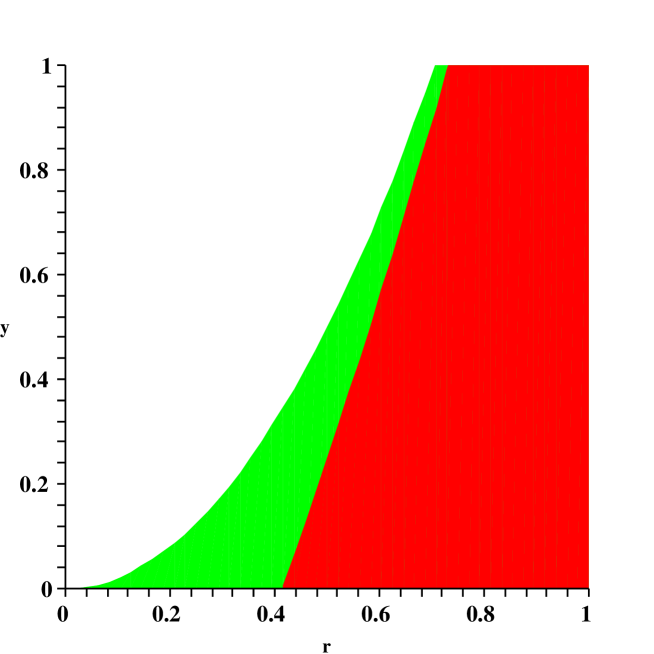
    Figure 1: The admissible 2-tensor domain in a $\left(r,T_{4}\right)$-plot.

    It is more convenient to introduce new variables

    $$\left(r,T_{4}\right)\longrightarrow\left(r,z=\frac{1}{2}-\sqrt{2r^{2}-T_{4}}\right),$$

    the inequalities (37) now read

    $$\frac{1}{2}-z\leq r\leq\frac{1}{2}+z\quad 0\leq z\leq\frac{1}{2}$$

    $$\frac{1}{2}+z\leq r\leq\frac{1}{2}-z\quad-\frac{1}{2}\leq z\leq 0.$$

    In terms of the $N_{m}:=m\left(2m-1\right)$ matrix elements of $G^{\{m,2\}}$ the invariants $r,T_{4}$ or $r,z$ correspond to the following geometrical ’balls’

    For all $$m$$ we have

    $$r=\sum_{i<j}^{2m}\left(G^{\{m,2\}}_{i,j}\right)^{2}$$

    i.e. the $$\left(N_{m}-1\right)$$-sphere of the Frobenius norm (38)

    $$\text{For $m=2$}:$$

    a straightforward calculation shows

    $$2r^{2}-T_{4}=\frac{1}{16}\text{trace}\left(\tilde{G}^{\{2,2\}}.G^{\{2,2\}}\right)^{2}$$ (39)

    where

    $$\tilde{G}^{\{2,2\}}\text{ is the dual tensor }\;\tilde{G}^{\{2,2\}}_{i_{1},i_{2}}=\epsilon_{i_{1},i_{2},i_{3},i_{4}}G^{\{2,2\}}_{i_{3},i_{4}}.$$

    ($\tilde{A}:=\tilde{G}^{\{3,2\}}\text{ the tensor dual to }G^{\{3,2\}}$)

    For $$m=3$$ we find

    $$2r^{2}-T_{4}=\frac{1}{16}\|\tilde{A}\|^{2}=\frac{1}{32}\text{trace}\left(\tilde{A}^{T}\tilde{A}\right)$$ (40)

    $$\|\tilde{A}\|\text{ is the Frobenius norm of the 2-tensor (32).}$$

  The parameters $a_{i,k}:=G^{\{m,2\}}_{i,k}$ are seen to lie in generalized elliptic ’tunnel’ domains (see below). In detail we have

  • $m=2$:
    Expressing $z$ in terms of $a_{i,k}$

    $$z=\frac{1}{2}-2\,|a_{1,2}a_{3,4}+a_{1,3}a_{4,2}+a_{1,4}a_{2,3}|$$ (41)

    $$\text{remember}\quad\lambda=\frac{1}{4}\left(1\pm\sqrt{r\pm\left(\frac{1}{2}-z\right)}\right)$$

    we shall see that the admissible values $-\frac{1}{2}\leq z\leq\frac{1}{2}$ lie in a generalized elliptic ’tunnel’ domain embedded in $\mathbb{R}^{6}$.

  • $m=3$:
    The analogeous expression reads in this case

    $$z= \frac{1}{2}-2\left(\left(a_{4,5}a_{3,6}-a_{4,6}a_{3,5}+a_{3,4}a_{5,6}\right)^{2}\right.$$ (42)

    $$\left.+\left(a_{2,5}a_{4,6}-a_{4,5}a_{2,6}+a_{2,4}a_{3,6}\right)^{2}\right.$$

    $$\left.+\text{ thirteen similar terms }\right)^{1/2}$$

    and $z=z\left(a_{i,k}\right)$ is the ’tunnel’ domain embedded in $\mathbb{R}^{15}$ which we shall illustrate at the end of the section.

• I should include a short discussion of a qualitative method for the construction of $O\left(2m\right)$-invariants by inference. First of all we assign the scale dimension $\delta=1$ to the tensor $G^{\{m,k\}}\text{ all }m,k$. The eigenvalues then have $\delta=1$, the characteristic polynomial $P\left(z\right)=\sum_{i=0}^{d}c_{i}z^{i}$ of degree $d$ has $\delta=d$, the coefficients have $\delta^{d-i}$. Hence $c_{i}$ is composed of invariants of scale dimension $\leq d-i$ (counting dimensions such that by putting $G^{\{m,0\}}=1$ (and thus fulfilling the normalisation condition) we mean that unity carries one dimensional unit). In detail we have the following invariants

  • $\delta=d=4$ : $T_{4}$ and $r^{2}$.
    We reiterate the identities introduced above.
    $m=2$:

    $$2r^{2}-T_{4} =\frac{1}{16}\left(\epsilon_{i_{1},i_{2},i_{3},i_{4}}G^{\{2,2\}}_{i_{1},i_{2}}G^{\{2,2\}}_{i_{3},i_{4}}\right)^{2}$$

    $$=4\,\text{Determinant}\left(G^{\{2,2\}}\right)$$ (43)

    m=3:

    $$2r^{2}-T_{4}=$$

    $$\frac{1}{32}\epsilon_{i_{1},i_{2},i_{3},i_{4},i_{6},i_{5}}G^{\{3,2\}}_{i_{1},i_{2}}G^{\{3,2\}}_{i_{3},i_{4}}\epsilon_{i_{5},i_{6},i_{7},i_{8},i_{9},i_{10}}G^{\{3,2\}}_{i_{7},i_{8}}G^{\{3,2\}}_{i_{9},i_{10}}$$ (44)

  • $\delta=3$ : The invariants are the $D^{\left(3\right)}$ discussed above.

  • $\delta=2$ : The only invariant is $r$ defined above.

  • $\delta=1$ : $G^{\{m,0\}}$
    Normalisation forces the only invariant, the scalar $G^{\{m,0\}}=1$, to be counted with $\delta=1$. The term of order $\lambda^{0}$, the invariant $D^{\left(3\right)}$, should be read as $\left(D^{\left(3\right)}.G^{\{3,0\}}\right)$.

• Visualisation of ’tunnel’ domains:
  We now now illustrate the domains for the matrix elements $G^{\{m,2\}}_{i,k}$ prescribed by the probability interpretation of the eigenvalues (31) (as a reminder, these formulae hold exactly for $m=2$ and for $m\geq 3$ when we demand certain scalar products of pseudo-tensor(vector) configurations vanish, $D^{\left(3\right)}$ for $m=3$). For obvious reasons we restrict the configurations to three non-vanishing matrix elements, e.g.

  $$G^{\{m,2\}}_{1,2}:=x\quad G^{\{m,2\}}_{3,4}:=y\quad G^{\{m,2\}}_{2,3}:=z$$

  $$G^{\{m,2\}}_{i,k}:=0\quad\text{otherwise}.$$

  The eigenvalues then are

  $$\lambda_{1,2}=\frac{1}{4}\left(1\pm\alpha_{+}\right)$$ (45)

  $$\lambda_{3,4}=\frac{1}{4}\left(1\pm\alpha_{-}\right)$$ (46)

  where

  $$\alpha_{\pm}=\sqrt{\left(x\pm y\right)^{2}+z^{2}}.$$ (47)

  The domains are determined by the inequalities

  $$0\leq\alpha_{+}\leq 1\;\;\wedge\;\;0\leq\alpha_{-}\leq 1;$$

  the admissible domains have to be subsets of these parameter regions which graphically represent two ’orthogonal’ ’tunnels’ with symmetry axes $y=\pm x$ and elliptic cross sections, half-axes $1\text{ and }\sqrt{\frac{1}{2}}$ as depicted in Figure 2.

  

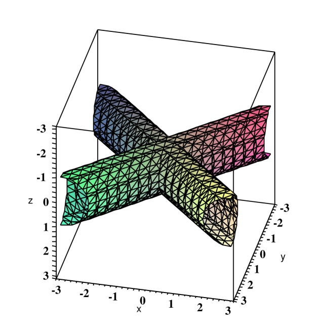
  Figure 2: The domains (47) as a function of unrestricted $\{x,y,z\}$

  The physical domain is finally constructed as the intersection $\mathfrak{Int}=\text{tunnel}_{\alpha_{+}}\cap\text{tunnel}_{\alpha_{-}}\cap\{[x,y,z]|0\leq x,y,z\leq 1\}$ where the last set, the cube with edges $[x_{0},y_{0},z_{0}],\;\;x_{0},y_{0},z_{0}=0,1$ represents the positivity condition, the correct normalisation is guaranteed by (45) and (46). Figure 3 illustrates this intersection.

  

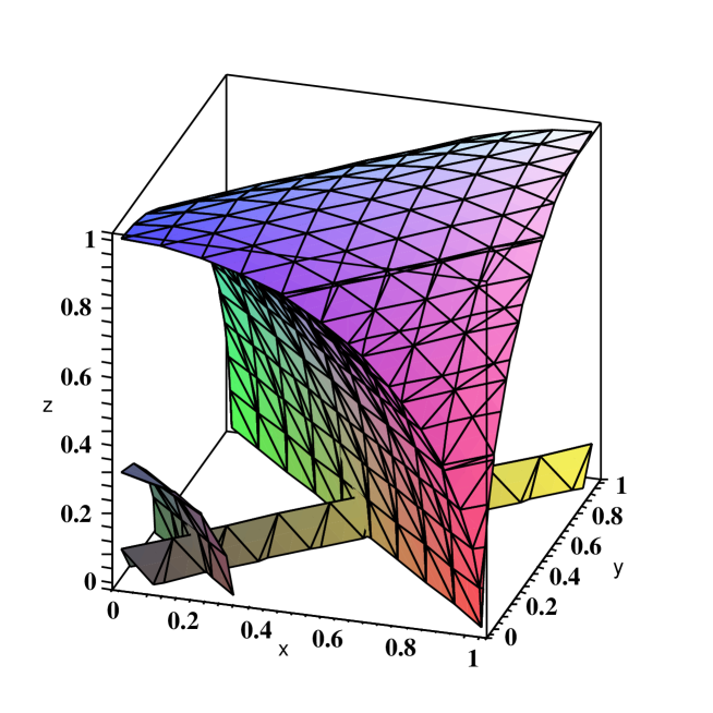
  Figure 3: The intersection $\mathfrak{Int}:$ surfaces $\alpha_{+}=1.\text{ and }\,0.1$ ; $\,\alpha_{-}=1.\text{ and }\,0.01$ are depicted.

5 An Alternative Parameter Classification

In the following I shall describe a classification which has the charm of accommodating a larger set of parameters into one tensor representation but is algebraically incomplete. Whether this has disadvantages when it comes to physical applications can be decided only after a clarification of the rôle of discrete transformations (similar to Parity and Charge conjugation in Dirac theory). We postpone such questions and proceed as follows.
Put

$$\check{\Gamma}^{\{m,1\}}:=[\,\hat{\Gamma}^{\{m,1\}}_{1},\ldots,\hat{\Gamma}^{\{m,1\}}_{2m},\Gamma^{\{m\}}_{2m+1}\,].$$

Then as already stated the $\check{\Gamma}^{\{m,1\}}_{i}$ fulfil the anti-commutation relations

$$\check{\Gamma}^{\{m,1\}}_{i}.\check{\Gamma}^{\{m,1\}}_{j}+\check{\Gamma}^{\{m,1\}}_{j}.\check{\Gamma}^{\{m,1\}}_{i}=2\,\delta_{i,j}\mathbb{I}$$ (48)

$$i,j=1\ldots 2m+1.$$

Following equations (5) and (6) we write

$$\check{\Gamma}^{\{m,k\}}_{i_{1}\ldots i_{k}}=F_{Norm}^{\{m,k\}}\;\left(\varepsilon_{i_{1}\ldots i_{2m}}\;\check{\Gamma}^{\{m\}}_{i_{k+1}}.\ldots\check{\Gamma}^{\{m\}}_{2m}\right).$$

The $2^{m}-1$ parameters of an m-Qubit are then accommodated in the expansion

$$\varrho^{m-Qubit}=\sum_{k=0}^{m}\check{G}^{\{m,k\}}\circ\check{\Gamma}^{\{m,k\}}$$

where it is essential to note

$$\sum_{k=0}^{m}\binom{2m+1}{k}=2^{2m}$$

the number of matrix elements defining the state $$\varrho$$.

The point to keep in mind is of course that this expansion is incomplete. However depending on the rôle of the already mentioned ’P’-, ’C’-transformations duality relations among the $\{m,k_{0}\}$ and $\{m,2m-k_{0}\}$ tensors will resolve this problem.
This scheme takes care of a larger number of parameters

$${\bf m=2:}$$

$$\text{Number of parameters }=\begin{cases}5\quad\qquad\,\left(4\right)\,\,&\text{ for }k=1\quad\text{ Vector}\\ 5+10\quad\left(4+6\right)\,\,&\text{ for }k=2\quad\text{2-Tensor}\end{cases}$$

$${\bf m=3:}$$

$$\text{Number of parameters }=\begin{cases}7\quad\qquad\,\left(6\right)\,\,&\text{ for }k=1\quad\text{ Vector}\\ 7+21\quad\left(6+15\right)\,\,&\text{ for }k=2\quad\text{ 2-Tensor}\end{cases}$$

We now calculate the vector and 2-tensor spectra for this new representation:
for k=1 the problem is already solved, see (38) and (39)
for k=2 we have
m=2: the formulae (31)

$$\lambda=\frac{1}{4}\left(1\pm\sqrt{r\pm\sqrt{2r^{2}-T_{4}}}\right),$$

as well as (32) and (33) hold with the replacement $G^{\{m,2\}}\longrightarrow\check{G}^{\{m,2\}}$
m=3: The same formulae hold if we replace the condition

$$D^{\left(3\right)}=0$$ (49)

by

$$\text{the $\;O\left(2m+1\right)$-invariant }\;\sum_{i=1}^{6}V_{i}^{2}=0$$ (50)

$$\text{i.e. }V_{i}=0\quad i=1\ldots 7$$

with

$$V_{i}=\epsilon_{i,i_{1},\ldots,i_{6}}\check{G}^{\{3,2\}}_{i_{1},i_{2}}\check{G}^{\{3,2\}}_{i_{3},i_{4}}\check{G}^{\{3,2\}}_{i_{5},i_{6}}.$$ (51)

Note that $V_{7}=D^{\left(3\right)}$. For $m\geq 4$ the situation is a bit more involved. The corresponding maps (sub-’pseudovectors’)

$$\mathbb{M}\left(\mathbb{R},2m\right)_{i}\rightarrow\mathbb{R}\quad i=1\ldots 2m+1$$

of scale dimension $m$ constructed analogously to (51):

$$V_{i_{1}}=\epsilon_{i_{1},\ldots,i_{2m+1}}\;\,\check{G}^{\{m,2\}}_{i_{2},i_{3}}\ldots\check{G}^{\{m,2\}}_{i_{2m},i_{2m+1}}$$

carry too high dimension and play no rôle on the 2-tensor level. Suitable ’pseudo-tensors’ have to be constructed and contracted to (pseudo-)scalars of the required dimension $6$. The normalisation of states is fixed once and for ever by normalising the scalar term, positivity is guaranteed by the same inequalities among now $O\left(2m+1\right)$-invariants obtained above.

6 Summary

Given a hermitian matrix with unit trace the decision whether or not it is a state is not at all trivial. More precisely speaking the a priori construction of a matrix representation of a state, a density matrix, is non-trivial. The classic way to determine the eigenvalues of this matrix as a function of its matrix elements, to solve the characteristic equation, is in general feasible (by radicals and algebraic operations) only for dimension$\leq 4$. For higher dimensions e.g. the Descartes’ rule can be applied to derive admissible parameter domains. Doublet ($m=1$), quartet ($m=2$), and eventually octet ($m=3$) structures in m-Qubit spectra can be handled in this way with tolerable effort. Therefore a systematic study of generacy structures in m-Qubit spectra seems essential.
The key of the approach we followed is to embed m-Qubit states in Clifford algebras $\mathfrak{Cl}_{2m}$. The construction of a basis of this algebra from Clifford numbers obeying the anti-commutation rules (1) and (48) leads, considering the dual representation (9) of the algebra, to a classification of states as $O\left(2m\right)$- or $O\left(2m+1\right)$-tensors; the eigenvalues of these states are functions of $O\left(2m\right)$- and $O\left(2m+1\right)$-invariants. The number of parameters controlling positivity is thus considerably reduced. For m-Qubits the case of degeneracy into doublets leads to a vector classification: state-parameters lie on $\left(2m-1\right)$- or $2m$-Bloch spheres. The degeneracy into quartets leads to more involved structures: relations among invariants and their embedding in parameter spaces are dicussed in some detail. $m\left(2m\mp 1\right)$-dimensional intersections of ’tunnel’-like objects with elliptic cross-sections appear as generalisations of Bloch spheres. Progressing to tensors with $k_{0}\geq 3$ one immediately encounters the obstacle of not explicitly knowing the eigenvalues as functions of $O\left(2m\left(+1\right)\right)$-invariants, the already mentioned Descartes rule then comes into play.
The use of direct products of Qubit states as basis in m-Qubit state spaces has been proven useful for the development of criteria of separability, see e.g. [5], [6], [7], [8], [9]. Of particular interest in the present context are [2], [3] and references cited in these papers. There the basis $\{B_{i}\}$ is chosen as the generators of $SU\left(2^{m}\right)$, domains of admissible ’coherence vectors’ guaranteeing positivity of the density matrix of an m-Qubit are given in terms of Casimir invariants. In particular cases degeneracies were detected and the corresponding local unitaries described. Deriving explicit domains within this formalism soon encounters considerable problems (notwithstanding the essential structural clarifications gained): to determine the admissible domain for a m-Qubit one obtains $2^{m}-1$ polynomial inequalities with maximal degree $2^{m}$: writing the characteristic polynomial as $P\left(\lambda\right)=\sum_{i=1}^{2^{m}}\left(-1\right)^{i}a_{i}\lambda^{i}\quad$ $a_{2^{m}}$ is of scale dimension $2^{m}$ in the ’coherence vector’ $\vec{n}$, (scale dimemsion($a_{i}$)$=i$); the necessary and sufficient condition for positivity of the density matrix $a_{i}>0\text{ for all i },\;\;a_{i}=a_{i}\left(\vec{n}\right)$.
The approach we follow leads to a $O\left(2m\left(+1\right)\right)$-tensor classification and the corresponding degeneracy patterns. Domains of admissible parameters can thus be derived for all $m$ with increasing complexity for increasing order of the $O\left(2m\left(+1\right)\right)$-tensors (the $k_{tensor}=1,2,3$ cases can be comfortably handled on a standard laptop).

References

• [1] Pertti Lounesto,
Clifford Algebras and Spinors, Second Edition,
Cambridge University Press 2001
Ablamowicz, R.,
Lectures on Clifford (Geometric) Algebras and Applications.
Birkhaeuser, Basel 2003
Snygg, J.
Clifford Algebra, Computational Tool for Physicists.
Oxford University Press 1997
Herrmann, R.
Spinors, Clifford and Cayley Algebras
Interdisciplinary Mathematics Vol.7, New Brunswick
• [2] Byrd, M.S., and Khaneja,N.
Characterisation of the positivity of the density matrix in terms of the coherence representation
Phys.Rev. A 68 062322 (2003)
• [3] Kimura, G.
The Bloch Vector for N-Level Systems
quant-ph/0301152
• [4] For an alternative discussion of geometric aspects of the problem of constructing states see
KΓΊs, M. and Zyczkowski, K.
Geometry of Entangled States
Phys.Rev. A63 032307 (2001)
• [5] Aschauer, H., Calsamiglia, J., Hein, M., and Briegel, H.
Local invariants for multi-partite entangled states allowing for a simple entanglement criterion
quant-ph/0306048
• [6] Jaeger, G., Teodorescu-Frumosu, M., Sergienko, A., Saleh, B.E.A., and Teich, M.C.
Multi-photon Stokes-parameter invariant for entangled states
Phys.Rev. A67 032307 (2003)
• [7] Linden, N., and Popescu, S.
On multi-particle entanglement
Fortschr.Physik 46 567 (1998)
• [8] Schlienz, J., and Mahler, G.
Description of entanglement
Phys.Rev. A52 4396 (1995)
• [9] Hioe, F.T., and Eberly, J.H.
n-level coherence vector and higher conservation laws in quantum optics and quantum mechanics
Phys.Rev.Lett. 47 838 (1981)