Opposites Attract - A Theorem About The Casimir Force

Abstract

We consider the Casimir interaction between (non-magnetic) dielectric bodies or conductors. Our main result is a proof that the Casimir force between two bodies related by reflection is always attractive, independent of the exact form of the bodies or dielectric properties. Apart from being a fundamental property of fields, the theorem and its corollaries also rule out a class of suggestions to obtain repulsive forces, such as the two hemisphere repulsion suggestion and its relatives.

The Casimir effect has been a fundamental issue in quantum physics since its prediction Casimir48 . The effect has become increasingly approachable in recent years with the achievement of precise experimental measurements of the effect Sparnaay59 ; Lamoreaux97 ; MohideenRoy98 ; Bressi , probing the detailed dependence of the force on the properties of the materials, and measuring new variants such as corrugation effects. The theory and experiment have good agreement for simple geometries.

In spite of the vast body of work on the subject (For a review see BordagMohideenMostepanenko ), some properties of the force are yet under controversy. Due to the computational complexity of the problem, the main body of work on the effect is a collection of explicit calculations for simple geometries. In this Letter we resolve one of these controversies and supply general statements about Casimir forces, applicable to a broad class of geometries.

The interest in repulsive Casimir and Van Der Waals forces has grown substantially recently due to possible practical importance in nano science, where such forces may play a role as a solution to stiction problems. It is known that repulsive forces are possible between molecules immersed in a medium whose properties are intermediate between the properties of two polarizable molecules Isra . Conditions for repulsion between paramagnetic materials and dielectrics without recourse for an intermediate medium were given in KennethKlich . However, the prospect of realizing materials with nontrivial permeability on a large enough frequency range is unclear IannuzziAndReply .

It is common knowledge, based on the Casimir-Polder interaction, that small dielectric bodies interacting at large distance attract kn . Based on summation of two body forces one may speculate that any two dielectrics would attract at all distances. In this Letter we show that at least for the case of a symmetric configuration of two dielectrics or conductors this prediction holds independently of their distance and shape, for models which can be described by a local dielectric function. Of course, in any real material as distances become small enough, i.e. compared with interatomic distances, Casimir treatment of the problem is not adequate anymore.

We first emphasize that the two-body picture is not enough to prove this. Calculations of the interaction between macroscopic bodies by summation of pair - interactions are only justified within second order perturbation theory. Indeed, in KennethKlich it was demonstrated how summing two body forces may give wrong prediction for the sign of interaction between extended bodies.

Another objection to the pair-wise intuition is based on the example of Casimir energy of a perfectly conducting and perfectly thin sphere. This was worked out by Boyer Boyer and yields an outward pressure on the sphere. This result motivated a class of suggestions for repulsive forces, the most well known of which are two conducting hemispheres - considered as a sphere split into two and therefore expected to repel each other Lamoreaux97 ; ElizaldeRomeo (Fig. 1).

One may try to use perturbative series, such as the multiple scattering series in the conducting case BalianDuplantier78 and show the attraction term by term. However, checking such a claim at orders higher then second might prove a difficult task. Such an approach is justified for distant bodies, but doesn’t seem to be particularly promising for the problem at hand.

Our main result is that the electromagnetic field (EM) or a scalar field, interacting with (non-magnetic) bodies, which are mirror image of each other and separated by a finite distance, will cause the bodies to attract. In particular, this shows that two hemispheres attract each other. The result holds for a scalar field in any dimension and even when the bodies are inside an infinite cylinder of arbitrary cross-section (perpendicular to the reflection plane) with arbitrary boundary conditions (b.c.) on the cylinder, thereby verifying and generalizing recent results for a Casimir piston HertzbergJaffeKardarScardicchio .

Expressing the Casimir interaction as a (regular) determinant. Several expressions are available for Casimir forces between dielectrics. We find the path integral method LiKardar ; Kenneth99 ; FeinbergMannRevzen a convenient starting point for the presentation (alternatively, the result may be obtained using other approaches such as the Green’s function method). We start with the case of a scalar field for simplicity, and explain later how the result is extended to the EM field.

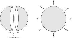
Figure 1: What is the direction of the force between two conducting hemispheres? While the outward pressure on a conducting shell might suggest repulsion, it follows from the arguments below that the hemispheres in fact attract

The action of a real massless scalar field in the presence of dielectrics can be written as

$$S={1\over 2}\int{\rm d}^{d}{\bf r}\int{{\rm d}\omega\over 2\pi}\phi_{\omega}^{*}(\nabla^{2}+\omega^{2}\epsilon({\bf x},\omega))\phi_{\omega}$$ (1)

where $\phi_{\omega}^{*}=\phi_{-\omega}$, and $\epsilon(\omega,{\bf x})=1+\chi({\bf x},\omega)$ is the dielectric function (we use units $\hbar=c=1$). The change in energy due to introduction of $\chi$ in the system is formally:

$$E_{C}=E_{\chi}-E_{\chi=0}=\\ -i\int_{0}^{\infty}{{\rm d}\omega\over 2\pi}\log{\det}_{\Lambda}(1+\omega^{2}\chi({\bf x},\omega)(\nabla^{2}+\omega^{2}+i0)^{-1})$$

A determinant is mathematically well defined if it has the form $\det(1+A)$, where $A$ is a ”trace class” operator, i.e. $\sum_{i}|\lambda_{i}|<\infty$ with $\lambda_{i}$ eigenvalues of $A$ (For properties see Simon79 ). The expression above is not of this form, and only has meaning when specifying cutoffs. Removing physical cutoffs will leave us with an ill defined determinant and so we keep in mind cutoffs at high momenta in the notation $\det_{\Lambda}$ (one may use instead lattice regularization).

At high frequencies $\chi(\omega,{\bf x})\rightarrow 0$, provides a physical frequency cutoff. $\chi(\omega)$ and $(\nabla^{2}+\omega^{2}+i0)$ are analytic for ${\rm Re}\omega,{\rm Im}\omega>0$, justifying Wick-rotation of the integration to the imaginary axis $i\omega$ ending up with:

$$E_{C}=\int_{0}^{\infty}{{\rm d}\omega\over 2\pi}\log{\det}_{\Lambda}(1+\omega^{2}\chi({\bf x},i\omega)G_{0}({\bf x},{\bf x}^{\prime}))$$ (2)

Where ${G_{0}}({\bf x},{\bf x}^{\prime})=\langle{\bf x}|{1\over-\nabla^{2}+\omega^{2}}|{\bf x}^{\prime}\rangle$. Restricting the operator $(1+\omega^{2}\chi G_{0})$ to the support of $\chi$ (more precisely to $L^{2}(Supp(\chi))$) clearly does not affect its determinant. We assume $\chi$ is nonzero only inside the volumes of the two dielectrics $A,B$ and we therefore consider in the following $(1+\omega^{2}\chi G_{0})$ as an operator on ${H_{A}\oplus H_{B}}\rightarrow{H_{A}\oplus H_{B}}$ where $H_{A}=L^{2}(A)$ and $H_{B}=L^{2}(B)$. It is then convenient to write it as $(1+\omega^{2}\chi G_{0})\Big{|}_{H_{A}\oplus H_{B}}=\left(\begin{array}[]{cc}1_{A}+\omega^{2}\chi_{A}{G_{0}}_{AA}&\omega^{2}\chi_{A}{G_{0}}_{AB}\\ \omega^{2}\chi_{B}{G_{0}}_{BA}&1_{B}+\omega^{2}\chi_{B}{G_{0}}_{BB}\\ \end{array}\right)$. It turns out that the part of the energy that depends on mutual position of the bodies, and as such is responsible for the force, is a well defined quantity, independent of the cutoffs. To see this, we subtract contributions which do not depend on relative positions of the bodies $A,B$:

$$E_{C}=E_{C}(A\bigcup B)-E_{C}(A)-E_{C}(B)$$ (3)

As in FeinbergMannRevzen this amounts to subtracting the diagonal contributions to the determinant which are not sensitive to the distance between the bodies, (i.e. only contributes to their self energies). This yields:

$$E_{C}=\int_{0}^{\infty}{{\rm d}\omega\over 2\pi}\Big{\{}\log{\det}_{\Lambda}\left(\begin{array}[]{cc}1+\omega^{2}\chi_{A}{G_{0}}_{AA}&\omega^{2}\chi_{A}{G_{0}}_{AB}\\ \omega^{2}\chi_{B}{G_{0}}_{BA}&1+\omega^{2}\chi_{B}{G_{0}}_{BB}\\ \end{array}\right)\\ -\log{\det}_{\Lambda}\left(\begin{array}[]{cc}1+\omega^{2}\chi_{A}{G_{0}}_{AA}&0\\ 0&1+\omega^{2}\chi_{B}{G_{0}}_{BB}\\ \end{array}\right)\Big{\}}\\ =\int_{0}^{\infty}{{\rm d}\omega\over 2\pi}(\log{\det}_{\Lambda}\left(\begin{array}[]{cc}1&T_{A}{G_{0}}_{AB}\\ T_{B}{G_{0}}_{BA}&1\\ \end{array}\right)$$ (4)

where $T_{\alpha}={\omega^{2}\over 1+\omega^{2}\chi_{\alpha}{G_{0}}_{{\alpha}{\alpha}}}\chi_{\alpha}$. Finally, using the relation $\det\left(\begin{array}[]{cc}1&X\\ Y&1\\ \end{array}\right)=\det(1-YX)$, which holds for block matrices we have:

$$E_{C}(a)=\int_{0}^{\infty}{{\rm d}\omega\over 2\pi}\log\det(1-T_{A}{G_{0}}_{AB}T_{B}{G_{0}}_{BA}).$$ (5)

Note that the (hermitian) operators $T_{\alpha}$ are exactly the $T$ operators appearing in the (Wick rotated) Lippmann-Schwinger equation scattering books . Indeed, one may alternatively derive Eq. (5) within Green’s function approach and using $T$ operators.

In (5) we disposed of the cutoff $\Lambda$ as the expression is well defined in the continuum limit. We recall that an operator $M$ is called positive (denoted $M>0$) if $\langle\psi|M|\psi\rangle>0$ for any $\psi$. Since $\chi(i\omega,x)>0$ (as follows from general properties of the dielectric function LifsitzPitaevskii ), the $T$ operators are positive and bounded, and $T_{A}{G_{0}}_{AB}T_{B}{G_{0}}_{BA}$ is a trace class operator without need for cutoffs for any finite bodies $A,B$ . In fact, this holds also for nonlocal $\chi$ as long as $f(x)\rightarrow\int_{A}\chi(i\omega,x,x^{\prime})f(x^{\prime}){\rm d}x^{\prime}$ is a bounded positive operator $H_{A}\rightarrow H_{A}$. At this point the determinant is regularized and rigorously well defined for every $\omega$ and the integration over $\omega$ is convergent due to the exponential decay of the kernels ${G_{0}}_{AB}$ as $\omega\rightarrow\infty$.

It is worthy to note that (for $\chi>0$) all eigenvalues $\lambda$ of the (compact) operator $T_{A}{G_{0}}_{AB}T_{B}{G_{0}}_{BA}$ appearing in (5) satisfy $1>\lambda\geq 0$ .

The Theorem.

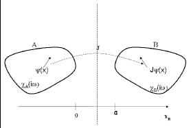
Figure 2: Bodies $A$ and $B$ are related by the reflection $J$

Having established a mathematically well defined expression for the Casimir energy, we now come to the main result: Consider a configuration of two bodies $A,B$ related by a reflection (Fig. 2), with $\chi(i|\omega|)$ a bounded positive operator and separated by a finite distance $a$; then (for fixed spatial orientations of the bodies) $E_{C}$ given in (5) is a monotonically increasing function of $a$ (i.e. the Casimir force is attractive).

Proof: We assume that $A$ is located entirely in the negative $x_{n}$ half space, and that $B$ is its mirror image under reflection through the $x_{n}=a/2$ plane. To exploit the reflection symmetry we introduce a mapping $J:A\rightarrow B$ given by $J({\bf x}_{\perp},x_{n})=({\bf x}_{\perp},a-x_{n})$. Note that $B=JA$. $J$ is volume preserving and induces a unitary operator ${\cal J}:H_{A}\rightarrow H_{B}$ defined by ${\cal J}\psi({\bf x})=\psi(J({\bf x}))$. In the case that $\psi$ is a vector field, as in the EM case below we take ${\cal J}\psi({\bf x})=(\psi_{\perp}(J({\bf x})),-\psi_{n}(J({\bf x})))$ (see Fig. 2). Since the bodies $A,B$ are related by reflection we have $T_{B}={\cal J}T_{A}{\cal J}^{{\dagger}}$ and thus:

$$E_{C}=\int_{0}^{\infty}{{\rm d}\omega\over 2\pi}\log\det(1-T_{A}{G_{0}}_{AB}{\cal J}T_{A}{\cal J}^{{\dagger}}{G_{0}}_{BA})$$ (6)

Note that ${G_{0}}_{AB}{\cal J}={\cal J}^{{\dagger}}{G_{0}}_{BA}$ is a hermitian operator (this can be verified). The energy can therefore also be expressed as

$$E_{C}=\int_{0}^{\infty}{{\rm d}\omega\over 2\pi}\log\det\left(1-(\sqrt{T_{A}}{G_{0}}_{AB}{\cal J}\sqrt{T_{A}})^{2}\right)$$ (7)

We now show by a direct calculation that (as operators on $H_{A}$):

$${G_{0}}_{AB}{\cal J}>0$$ (8)

$$\partial_{a}{G_{0}}_{AB}{\cal J}<0$$ (9)

Let $I(a)=\langle\psi|{G_{0}}_{AB}{\cal J}|\psi\rangle$ for a function $\psi({\bf x}_{\perp},x_{n})\in H_{A}$. $I(a)$ is explicitly given by

$$I(a)=\int_{A\times A}{\rm d}{\bf x}{\rm d}{\bf x}^{\prime}\int{{\rm d}{\bf k}\over(2\pi)^{d}}\psi^{*}({\bf x})\psi({\bf x}^{\prime})\\ \times{e^{i{\bf k}_{\perp}\cdot({\bf x}_{\perp}-{\bf x}_{\perp}^{\prime})+ik_{n}(x_{n}+x_{n}^{\prime}-a)}\over{\bf k}^{2}+\omega^{2}}$$ (10)

Note that $x_{n}+x_{n}^{\prime}-a<0$, allowing integration over $k_{n}$ by closing a contour from below the real $k_{n}$ axis:

$$I(a)=\int_{A\times A}{\rm d}{\bf x}{\rm d}{\bf x}^{\prime}\int{{\rm d}{\bf k}_{\perp}\over(2\pi)^{d-1}}\psi^{*}({\bf x})\psi({\bf x}^{\prime})e^{i{\bf k}_{\perp}\cdot({\bf x}_{\perp}-{\bf x}_{\perp}^{\prime})}\\ \times{e^{\sqrt{{\bf k}_{\perp}^{2}+\omega^{2}}(x_{n}+x_{n}^{\prime}-a)}\over 2\sqrt{{\bf k}_{\perp}^{2}+\omega^{2}}}=\int{{\rm d}{\bf k}_{\perp}\over(2\pi)^{d-1}}{e^{-a\sqrt{{\bf k}_{\perp}^{2}+\omega^{2}}}\over 2\sqrt{{\bf k}_{\perp}^{2}+\omega^{2}}}\\ \times\Big{|}\int_{A}{\rm d}{\bf x}\psi^{*}({\bf x})e^{ik_{\perp}\cdot{\bf x}_{\perp}}e^{x_{n}\sqrt{{\bf k}_{\perp}^{2}+\omega^{2}}}\Big{|}^{2}$$ (11)

showing that $I(a)>0$, which proves (8), and that $\partial_{a}I(a)<0$ which proves (9).

From (8,9) it immediately follows that the operator $Y=\sqrt{T_{A}}{G_{0}}_{AB}{\cal J}\sqrt{T_{A}}:H_{A}\rightarrow H_{A}$ also satisfy $Y>0,\partial_{a}Y<0$. Hence a Feynman-Hellman argument implies that all its eigenvalues $1>\lambda_{n}(a)\geq 0$ are monotonically decreasing as functions of $a$. Since $\log\det(1-Y^{2})=\sum_{n}\log(1-\lambda_{n}^{2})$ is absolutely convergent it follows $\partial_{a}\log\det(1-Y^{2})>0$, and hence by (7) also $\partial_{a}E_{C}>0$.

This completes the proof for the scalar case.

To treat the EM case we start with the well known expression Eq. (80.8) of Lifshitz and Pitaevskii LifsitzPitaevskii for the change in free energy due to variation of the dielectric function $\epsilon$ at a temperature $T$:

$$\delta F=\delta F_{0}+{1\over 2}{T}\sum_{n=-\infty}^{\infty}\omega_{n}^{2}{\rm Tr}({\cal D}\delta\epsilon).$$ (12)

Here $F_{0}$ is the free energy due to material properties not related to long wavelength photon field, and $\omega_{n}=2\pi nT$ are Matsubara frequencies. ${\cal D}$ is the temperature Green’s function of the long wave photon field given by ${\cal D}(\vec{x},\vec{x^{\prime}},i\omega)_{ij}=<\vec{x}|{1\over\nabla\times\nabla\times+\omega^{2}\epsilon(r,i|\omega|)}|\vec{x}^{\prime}>_{ij}$

Eq(12) may be written as $\delta F=\delta F_{0}+\delta F_{C}$ where

$$F_{C}={1\over 2}{T}\sum_{n=-\infty}^{\infty}[\log{\det}_{\Lambda}(\nabla\times\nabla\times+\omega_{n}^{2}\epsilon(x,i\omega_{n}))$$ (13)

$$-\log{\det}_{\Lambda}(\nabla\times\nabla\times+\omega_{n}^{2})]$$

$$={1\over 2}{T}\sum_{n=-\infty}^{\infty}\log{\det}_{\Lambda}(1+\omega_{n}^{2}\chi(x,i\omega_{n}){\cal D}_{0}(i\omega_{n})).$$

where ${\cal D}_{0}(\vec{x},\vec{x^{\prime}},i\omega_{n})_{ij}=<\vec{x}|{1\over\nabla\times\nabla\times+\omega_{n}^{2}}|\vec{x}^{\prime}>_{ij}$. Note that $F_{C}$ is exactly the same as (Opposites Attract - A Theorem About The Casimir Force), with the scalar propagator $G_{0}$ replaced by the vector propagator ${\cal D}_{0}$.

Thus, starting with this expression, one repeats (3) and (4) to get (5), replacing $G_{0}$ by ${{\cal D}_{0}}$ everywhere (including in the definition of the $T$ operators). The analysis of the determinant now proceeds exactly as in the scalar case. The only place in the proof which needs to be modified is where the explicit form of $G_{0}$ was used i.e. Eq.(10), where we now have to use ${{\cal D}_{0}}_{ij}(k,i\omega)={1\over k^{2}+\omega^{2}}(\delta_{ij}+{k_{i}k_{j}\over\omega^{2}})$ instead.

The effect of using the vectorial propagator in Eq.(10) is to replace $\psi^{*}({\bf x})\psi({\bf x}^{\prime})$ by $\psi^{*}_{i}({\bf x})\psi_{j}({\bf x}^{\prime})(\delta_{ij}+{k_{i}k_{j}\over\omega^{2}})$. In the vectorial case ${\cal J}$ acts by ${\cal J}\psi({\bf x})=(\psi_{\perp}(J({\bf x})),-\psi_{n}(J({\bf x})))$ so we get a factor $(-1)^{\delta_{jn}}$. Substituting and integrating over $k_{n}$ as before we find

$$I_{vec}(a)=\pi\int{{\rm d}{\bf k}_{\perp}\over(2\pi)^{3}}{e^{-a\sqrt{{\bf k}_{\perp}^{2}+\omega^{2}}}\over\sqrt{{\bf k}_{\perp}^{2}+\omega^{2}}}\times\\ \left[(-1)^{\delta_{jn}}\phi^{*}_{i}\phi_{j}(\delta_{ij}+{k_{i}k_{j}\over\omega^{2}})\right]\Big{|}_{k_{n}=-i\sqrt{{\bf k}_{\perp}^{2}+\omega^{2}}}$$ (14)

where $\phi_{j}({\bf k}_{\perp})=\int_{A}{\rm d}{\bf x}\psi_{j}({\bf x})e^{-i{\bf k}_{\perp}\cdot{\bf x}_{\perp}}e^{x_{n}\sqrt{{\bf k}_{\perp}^{2}+\omega^{2}}}$. Now it is straightforward to check that the expression in square brackets is positive for any $\phi_{i}$ and the theorem follows.

Extensions and remarks:
1) Finite temperatures: As remarked above we have $\int{{\rm d}\omega\over 2\pi}\rightarrow T\sum_{\omega_{n}}$ at finite $T$. Since the positivity arguments apply to the determinant at each fixed imaginary frequency $\omega$, they will also hold at finite $T$.

2) Confined geometry in transverse directions Our theorem is easily extended to cover the case when placing the system inside an infinite cylinder, perpendicular to the $x_{n}=0$ plane, with arbitrary cross section. In this case, one has to replace our $G_{0}$ by the appropriate Helmholtz green’s function in the cylinder: $G_{0}(x,x^{\prime})=\int{\rm d}k_{n}\sum_{j}{\varphi_{j}({\bf x}_{\perp})\varphi_{j}^{{\dagger}}({\bf x^{\prime}}_{\perp})\over\omega^{2}+k_{n}^{2}+E_{j}}e^{ik_{n}(x_{n}-x_{n}^{\prime})}$, where $\varphi_{n}(x)$ are the appropriate quantized eigenmodes in the transverse direction, and the integration over ${\bf k}_{\perp}$ is replaced by discrete summation. Substituting this expression in the relevant integrals such as (11) yields the attraction. Since the attraction is independent of the $\varphi_{j}$, this result is independent of the b.c. one sets on the containing cylinder.

3) Dielectric in front of mirror Suggestions were raised for repulsion between arrays of dielectrics and a mirror plane GussoSchmidt04 , based on results for a rectangular cavity. Variation of our theorem shows that one actually has attraction. Consider the body $A$ to the left of a Dirichlet mirror located at $x_{n}=a/2$. By the image method the propagator is replaced by $G({\bf x},{\bf x^{\prime}})=G_{0}({\bf x}-{\bf x^{\prime}})-G_{0}({\bf x}+{\bf x^{\prime}}-a\hat{n})$. This may also be written as $G-G_{0}=-G_{0}{\cal J}$. It is then straightforward to arrive at the expression for the energy analogous to (5) with $\det(1-G_{0}{\cal J}T_{A})$ replacing $\det(1-G_{0}T_{A}G_{0}T_{B})$. Using similar considerations as in the proof above the attraction follows.

4) Dirichlet b.c.: Our approach never uses directly b.c. on the dielectrics; instead, we consider interaction with an arbitrary permittivity $\epsilon(x,\omega)$. This is adequate for describing real conductors. Idealized Dirichlet b.c. for a scalar field and ideal conductor b.c. for EM field are obtained as the limit of large $\chi(i\omega)$; However, Neuman b.c. do not follow from the present treatment, since they do not correspond to a positive perturbation, or indeed to any regular perturbation.

5) Nonpositive perturbations. Cases of effective $\chi<0$ typically occur when the medium between the bodies has higher permittivity then the bodies. These cases as well as cases with nontrivial magnetic permeability $\mu$ may be covered in a way similar to the above theorem. However conditions on $\chi,\mu$ must be specified to ensure that the eigenvalues of $1-T_{A}G_{0}T_{B}G_{0}$ remain positive. These conditions are related to the assumption that the perturbation may not be so negative as to introduce negative energy modes into the system.

Summary: Our main result is that the Casimir force between two dielectric objects, related by reflection, is attractive. Our theorem serves as a no-go statement for a class of suggestions for repulsive Casimir forces. Of course, the treatment is only valid at distances where the system may be described reliably in terms of the field and local dielectric functions alone. Although the above proof applies only to symmetric configurations, the approach presented here may be used to analyze the more general cases. A natural question rises: How far can our result be generalized? Which classes of interacting fields obey it?

I.K would like to thank L. S. Levitov R. L. Jaffe and A. Scaricchio for discussions. O.K. is supported by the ISF.

References

- (1) H. B. G. Casimir, Proc. Koninkl. Ned. Akad. Wet. 51, 793 (1948).
- (2) M. J. Sparnaay, Physica 25, 353 (1959);
- (3) S.K.Lamoreaux, Phys Rev. Lett. 78 5-8(1997);
- (4) Mohideen U and Roy A 1998 Phys. Rev. Lett. 81 4549
- (5) G. Bressi, G. Carugno, R. Onofrio and G. Ruoso, Phys. Rev. Lett. 88, 041804 (2002).
- (6) M. Bordag M., U. Mohideen and V.M. Mostepanenko, Physics Reports, vol.353, (no.1-3), Elsevier, (2001).
- (7) Jacob N. Israelachvili, Intermolecular and surface forces (Academic Press, London, 1992).
- (8) O. Kenneth, I. Klich, A. Mann and M. Revzen, Phys. Rev. Lett. 89 (2002) 033001
- (9) D. Iannuzi and F. Capasso, Phys. Rev. Lett. 91, 029101 (2003); O. Kenneth, I. Klich, A. Mann, and M. Revzen et al. Phys. Rev. Lett. 91, 029102 (2003)
- (10) O. Kenneth and S.Nussinov, Phys. Rev. D 65, 085014 (2002).
- (11) T. H. Boyer, Phys. Rev. 174, 1764 (1968)
- (12) E.Elizalde and A.Romeo, Am. J. Phys. Vol. 59. No.8 711(1991).
- (13) H. Li and M. Kardar, Phys. Rev. Lett. 67, 3275 (1991).
- (14) R. Balian and B. Duplantier, Ann. Phys.N.Y. 112, 165, (1978).
- (15) M. P. Hertzberg, R. L. Jaffe, M. Kardar, and A. Scardicchio Phys. Rev. Lett. 95, 250402 (2005)
- (16) O. Kenneth, preprint hep-th/9912102.
- (17) J. Feinberg, A. Mann and M. Revzen, Annals of Physics (New York) 288(2001)103-136
- (18) R. G. Newton, Scattering Theory of Waves and Particles, Springer Verlag, Berlin, 1982; D. B. Pearson, Quantum Scattering and Spectral Theory, Academic Press, London 1988.
- (19) E. M. Lifshitz and L. P. Pitaevskii, Statistical Physics, Pt. 2, Pergamon, Oxford, 1984.
- (20) B. Simon. Trace ideals and their applications, LMS vol 35. Cambridge, New York, NY, 1979.
- (21) A. Gusso and A. G. M. Schmidt, cond-mat/0410218