Irregular Dynamics in a Solvable One-Dimensional Quantum Graph

Abstract

We show that the quantum single particle motion on a one-dimensional line with Fülöp-Tsutsui point interactions exhibits characteristics usually associated with nonintegrable systems both in bound state level statistics and scattering amplitudes. We argue that this is a reflection of the underlying stochastic dynamics which persists in classical domain.

The advancement in nano-engineering in the last decade has brought novel incentives to the study of low-dimensional quantum systems with geometrically designed forms that have no counterpart in nature. The quantum graph, which is a generic one-dimensional model of nano-device composed of quantum wires, represents one of such systems EX96 ; KS99 . The interest to the quantum graph is enhanced with its possibility to emulate the two-dimensional system of quantum billiard EH05 , whose solution has required rather extensive numerical treatments. It is therefore quite appropriate, at this point, to investigate generic aspects and general features of quantum graphs ahead of detailed studies of specific models of nano-devices.

In a parallel development, quantum graphs have been used as a tractable model for the study of quantum chaos, or the irregular aspects of quantum dynamics occurring as quantum manifestations of classically chaotic systems KS97 ; KS00 . Naturally, it is expected that random quantum graphs, which are complex networks of quantum lines, would result in the universal quantum fluctuation that has been associated to the quantum chaotic dynamics KS01 ; GA04 . It has been revealed, however, that no real complex network is required for the irregular quantum dynamics to present itself. A very simple version of the quantum graph, the star graph, which is a quantum graph with many lines connected at a single node, has been shown to display the characteristics associated to partial quantum chaos in an analytical semiclassical study BK99 . A natural question to be asked is whether we can further simplify the model of quantum chaos to the point of solvability.

In this article, we consider one of the simplest possible quantum graph which is made up solely of nodes with two connected lines with the special property for the nodes called scale invariance. The resulting system amounts to a single one-dimensional line with number of scale invariant point interactions. We show that the system has elementary analytical scattering matrices and also elementary analytical eigenvalue equation, yet displays full characteristics of irregular quantum dynamics, both in scattering amplitudes and in bound state level statistics.

We discuss the implication of the results, and look into the apparent contradiction of the appearance of the quantum chaos in a seemingly integrable, solvable conservative one-dimensional system.

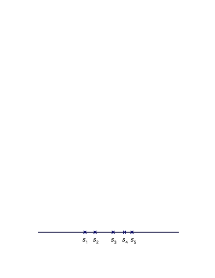
Figure 1: A schematic depiction of our model system. A free quantum particle moves along the line on which point interactions described by (3), (4) and (6) are located at $s_{1},\cdots,s_{N}$. This example shows the case of $N=5$.

We consider a quantum particle, constrained to move on a one-dimensional line with $N$ point-like defects AG88 whose locations are given by $x=s_{i}$ with $i=1,2,..N$ (FIG. 1). The Hamiltonian of the system is given, in appropriately rescaled unit, by

$$H=-\frac{1}{2}\frac{d^{2}}{dx^{2}}\quad{\rm on}$$ (1)

$$x\in(-\infty,s_{1})\cup(s_{1},s_{2})\cup...(s_{N-1},s_{N})\cup(s_{N},\infty).$$

The dynamics of the system is described by the Schrödinger equation

$$H\psi(x)=E\psi(x),$$ (2)

supplemented by the $U(2)$ connection conditions at the defects SE86 , which is conveniently specified FT00 by

$$(U_{i}-I)\Phi(s_{i})+iL_{0}(U_{i}+I)\Phi^{\prime}(s_{i})=0,$$ (3)

where $i$ runs as $i=1,2,...,N$, and $U_{i}$ is a unitary matrix belonging to $U(2)$ group. The boundary vectors $\Phi(x)$ and $\Phi^{\prime}(x)$ are given by

$$\Phi(s_{i})=\begin{pmatrix}\psi_{+}(s_{i})\\ \psi_{-}(s_{i})\\ \end{pmatrix},\quad\Phi^{\prime}(s_{i})=\begin{pmatrix}\psi^{\prime}_{+}(s_{i})\cr-\psi^{\prime}_{-}(s_{i})\end{pmatrix},$$ (4)

where $\psi_{\pm}(s_{i})$ and $\psi^{\prime}_{\pm}(s_{i})$ denote the limit value of $\psi(x)$ and its derivative from the upper and lower regions of the defects $s_{i}$, $x\to s_{i}\pm 0$. The constant $L_{0}$ is a length scale introduced to account for the scale anomaly JA95 inherent in one-dimensional point interaction. For technical simplicity, we assume all $U_{i}$ to be identical, $U=U_{i}$. Among all possible $U$, we consider scale invariant subfamily, discovered by Fülöp and Tsutsui FT00 whose $U$ has property

$${\rm det}[U\pm I]=0.$$ (5)

This condition guarantees the equation (3) without any involvement of the scale parameter $L_{0}$. The standard parametrization for this class of $U$ is

$$U=\begin{pmatrix}\cos\theta&e^{i\phi}\sin\theta\cr e^{i\phi}\sin\theta&-\cos\theta\end{pmatrix}.$$ (6)

This gives the connection condition which reads

$$\frac{e^{i\phi}}{\alpha}\psi_{-}(s_{i})=\psi_{+}(s_{i}),$$

$$e^{i\phi}\alpha\psi^{\prime}_{-}(s_{i})=\psi^{\prime}_{+}(s_{i}),$$ (7)

where the “strength” $\alpha$ is defined by

$$\alpha=-\cot\frac{\theta}{2}.$$ (8)

The Fülöp-Tsutsui point interaction (6) is a less known subclass of one-dimensional point interaction compared to the standard $\delta$ potential and $\delta^{\prime}$ (or $\varepsilon$) potential, but its property of scale invariance comes in handy in our following treatment. We stress that this seemingly exotic interaction is nevertheless realizable as a short-range limit of certain local potential CS98 . We first consider the scattering by a single defect. Let us, for a moment, suppose that there is only a single defect located at $x=s$. Considering the incoming wave from $x<s_{1}$ side, we assume the wave function to be in the form

$$\psi(x) = e^{ikx}-R_{1}(s_{i})e^{-ikx}\quad(x<s_{i}),$$ (9)

$$= T_{1}(s_{i})e^{ikx}\qquad\qquad\ \ (x>s_{i}).$$

We obtain the transmission and reflection amplitudes as

$$T_{1}(s_{i})=\frac{2\alpha}{1+\alpha^{2}}e^{i\phi},\quad R_{1}(s_{i})=\frac{1-\alpha^{2}}{1+\alpha^{2}}e^{2iks_{i}}.$$ (10)

For the scattering from $x>s_{N}$ side, we write

$$\psi(x) = T^{\prime}_{1}(s_{i})e^{-ikx}\qquad\qquad(x>s_{i}).$$ (11)

$$= e^{-ikx}-R^{\prime}_{1}(s_{i})e^{ikx}\quad(x<s_{i}),$$

and obtain

$$T^{\prime}_{1}(s_{i})=T^{*}_{1}(s_{i}),\quad R^{\prime}_{1}(s_{i})=-R^{*}_{1}(s_{i}).$$ (12)

The absence of the scale parameter $L_{0}$ results in the energy independence of scattering amplitude.

With elementary algebra, we can write the scattering amplitudes for $N$ defects in the recursive forms; For the left-right amplitudes $T_{N}$ and $R_{N}$, we have

$$T_{N}(s_{1},...,s_{N})=\frac{T_{1}(s_{1})T_{N-1}(s_{2},...,s_{N})}{1+R_{1}^{*}(s_{1})R_{N-1}(s_{2},...,s_{N})},\qquad$$

(13)

$$R_{N}(s_{1},...,s_{N})=\frac{R_{1}(s_{1})+R_{N-1}(s_{2},...,s_{N})}{1+R_{1}^{*}(s_{1})R_{N-1}(s_{2},...,s_{N})}.$$

The right-left amplitude $T^{\prime}$ $R^{\prime}$ are obtained from

$$T^{\prime}_{N}(s_{1},...,s_{N})=T_{N}^{*}(s_{N},...,s_{1}),$$

$$R^{\prime}_{N}(s_{1},...,s_{N})=-R_{N}^{*}(s_{N},...,s_{1}).$$ (14)

Note the reversed ordering of $s_{i}$ in right and left hand sides of the equations. With repeated iteration, we obtain explicit expressions for scattering matricesin the form

$$T_{N}(k)=\frac{\gamma^{N}}{D_{N}(k)},\quad R_{N}(k)=\frac{B_{N}(k)}{D_{N}(k)},$$ (15)

where $B_{N}(k)$ and $D_{N}(k)$ are defined by

$$\!\!\!\!\!\!\!\!B_{N}(k)={\beta\sum_{i}^{N}e^{2iks_{i}}+\beta^{3}\!\!\!\!\sum_{i>j>m}^{N}\!\!\!\!e^{2ik(s_{i}-s_{j}+s_{m})}+\beta^{5}\!\!\!\!\!\!\!\!\!\!\sum_{i>j>m>n>p}^{N}\!\!\!\!\!\!\!\!\!\!e^{2ik(s_{i}-s_{j}+s_{m}-s_{n}+s_{p})}+\cdots},$$ (16)

$$\!\!\!\!\!\!\!\!D_{N}(k)={1+\beta^{2}\sum_{i>j}^{N}e^{2ik(s_{i}-s_{j})}+\beta^{4}\!\!\!\!\!\!\sum_{i>j>m>n}^{N}\!\!\!\!\!\!e^{2ik(s_{i}-s_{j}+s_{m}-s_{n})}+\beta^{6}\!\!\!\!\!\!\!\!\!\!\!\!\sum_{i>j>m>n>p>q}^{N}\!\!\!\!\!\!\!\!\!\!\!\!e^{2ik(s_{i}-s_{j}+s_{m}-s_{n}+s_{p}-s_{q})}+\cdots},$$ (17)

and the abreviations

$$\beta=\frac{1-\alpha^{2}}{1+\alpha^{2}},\quad\gamma=\frac{2\alpha}{1+\alpha^{2}}e^{i\phi}$$ (18)

are used. The sum runs over all indices in the range between $1$ and $N$ with the specified constraint, and the numerator contains terms up to the order of $\beta^{[N/2]}$ where the exponent signifies the integer part of $N/2$. For given $N$, there are ${}_{N}C_{l}$ terms with order $\beta^{l}$, and the scattering matrices are the multi-periodic oscillatory functions with $2^{N-1}$ frequencies.

Along with scattering, we can also consider the bound spectra by limiting the system to finite line of size $L\geq s_{N}$. One of the easiest way is to impose Dirichlet boundary conditions at $x=-L$ and $x=L$, $\psi(L)=\psi(-L)=0$. This leads, for the case of $\phi=0$, to the eigenvalue equation

$$\left(R_{N}(k)-\!e^{-2ikL}\!\right)\left(R^{\prime}_{N}(k)-\!e^{-2ikL}\!\right)=T_{N}(k)T^{\prime}_{N}(k).$$ (19)

Explicite calculation again yields the form

$$\!\!\!\!\sin 2kL+\beta\sum_{i}^{N}\sin 2ks_{i}+\beta^{2}\sum_{i>j}^{N}\sin 2k(s_{j}\!-\!s_{i}\!+\!L)+\beta^{3}\!\!\!\sum_{i>j>m}^{N}\!\!\!\!\!\sin 2k(s_{m}\!-\!s_{j}\!+\!s_{i})$$

$$\qquad+\beta^{4}\!\!\!\!\!\sum_{i>j>m>n}^{N}\!\!\!\!\!\sin 2k(s_{n}\!-\!s_{m}\!+\!s_{j}\!-\!s_{i}\!+\!L)+\beta^{5}\!\!\!\!\!\sum_{i>j>m>n>p}^{N}\!\!\!\!\!\sin 2k(s_{p}\!-\!s_{n}\!+\!s_{m}\!-\!s_{j}+\!s_{i})+\cdots=0,$$ (20)

which is a bound state counterpart of (15).

In order to reveal the physical content of the scattering matrices (Irregular Dynamics in a Solvable One-Dimensional Quantum Graph) and the spectral function (19), we plot $|T_{N}|^{2}$ as the function of incident momentum $k$ for value of $\alpha=3/2$ in FIG.2. The number of point defects is set to be $N=3$, $N=5$ and $N=7$. The angle $\phi$ is set to be zero for all cases. The locations $s_{i}$ are set to be the sum of square root of primes; $s_{i}=\sum_{j=1}^{i}\sqrt{p_{j}}$, where $p_{j}$ stands for the $j$-th smallest prime with convention $p_{1}=1$, $p_{2}=2$. These values are selected to guarantee the incommensurability of $s_{i}$. This also models a generic case of random sequencing of successive $s_{i}$. We have checked that different choice of $s_{i}$, different ordering of relative size $s_{i+1}-s_{i}$ does not alter the essential characteristics of the results.

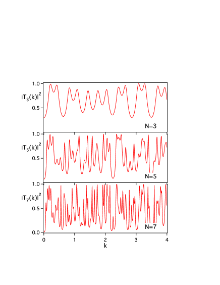
Figure 2: Transmission probability as the function of incident momentum. A common strengths parameter $\alpha=3/2$ is adopted. The location of the points are chosen to be $s_{1}=1$, $s_{2}=s_{1}+\sqrt{2}$, $s_{3}=s_{2}+\sqrt{3}$, $s_{4}=s_{3}+\sqrt{5}$ and $s_{5}=s_{4}+\sqrt{7}$, $s_{6}=s_{5}+\sqrt{11}$ and $s_{7}=s_{6}+\sqrt{13}$.

Despite the very simple analytic expression (15) of the scattering amplitude, as we increase $N$, the scattering quickly acquires “quantum chaotic” features BS88 , which is characterized by Ericson fluctuation ER60 , or the wild oscillation in scattering amplitudes caused by the overlapping resonances. Because of the scale invariance of the each point interactions, the fluctuation appears in arbitrary energy scale. Clearly, this fluctuation is the result of interferences among multi-periodic oscillations with incommensurate frequencies, whose number of periods $2^{N-1}$ proliferates very fast with increasing $N$.

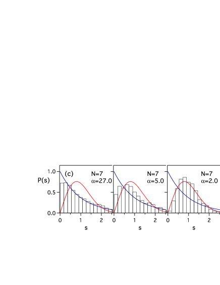
Figure 3: Nearest neighbor spacing distribution $P(s)$ obtained from the scaled energy levels of one-dimensional line limited to $x=[-L,L]$ with scale invariant point interactions. Location parameters $s_{i}$ are same, apart from the re-scaling, as in FIG. 2. Dirichlet boundary condition is imposed at both ends, $x=-L$ and $L$. The solid line represent the Wigner distribution $P(s)=\pi/2\cdot s\exp({-\pi/4\cdot s^{2}})$, and the dashed line the Poisson distribution $P(s)=\exp({-s})$.

We next examine the statistical properties of energy level sequence calculated from our system with periodic boundary condition. In FIG. 3, level spacing distribution $P(s)$ for the system with several $\alpha$ are shown for $N=3$, $N=5$, and $N=7$ cases from top to bottom as FIG3(a), FIG3(b) and FIG3(c). The distances $s_{i}$ are chosen to be $s_{i}-s_{i-1}:s_{i+1}-s_{i}=\sqrt{p_{i}}:\sqrt{p_{i+1}}$. The total length $L$ is set to be $s_{1}:2L$ $=1:\sum_{i=1}^{N+1}p_{i}$. We have chosen $\alpha=27$ to approximate disconnected large coupling limit, and $\alpha=2$ as the strong coupling limit, while, as an intermediate coupling, we chose the value $\alpha=5$. These graphs clearly show the approach of $P(s)$ to the Wigner distribution (also known as GOE distribution), which is regarded as the quantum signature of classically chaotic dynamics BG84 , at the strong coupling value as we increase the number of points $N$. The convergence appears to be fast as the Wigner-like level statistics already takes shape even with $N=3$. We have confirmed, with numerical calculations up to $N=19$, that very good convergence to the Wigner statistics is obtained with large $N$ if the coupling parameter $\alpha$ is properly rescaled to ensure the partial reflection/transmission of the system.

We now discuss the implication of our findings in a broader context. The central result of this article is the generation of the “random” or irregular properties in quantum dynamics out of fully analytic quantum spectral functions obtained from a one-dimensional system. This type of properties are usually associated to the nonintegrable system. Since the classical counterpart of conservative one-dimensional system necessarily is integrable, the well-established correspondence between the chaotic classical dynamics and the random quantum dynamics seems to fail for our model.

The clue to understand this seeming contradiction might be found in the singular nature of the high-energy limit of our system. Because of the special property of scale invariance present in Fülöp-Tsutsui point interaction, high energy limit, $k\to\infty$ does not bring the system to classical limit. As is well-known, high energy limit of $\delta$ and $\delta^{\prime}$ interactions corresponds to the free pass and perfect bouncing wall respectively, thus supplying two legitimate deterministic classical limits of a point interaction. With scale invariant point interactions, we are presented with semi-transparent wall with finite penetration probability at all energies. Therefore, if we were to identify the high energy limit as a classical limit, we are forced to consider stochastic dynamics whose randomness originates directly from the probabilistic nature of quantum mechanics itself.

Irrespective to the problem of classical limit and correspondence, our analytical expressions, made possible by the scale invariance of Fülöp-Tsutsui point interaction, shed light on how irregular quantum dynamics emerge as the infinite-period limit of multi-periodic scattering matrices, just as chaotic classical dynamics emerge as the infinite-period limit of multi-periodic motion. In this connection, it should be useful to consider a complementary approach of trace-formula based analysis to our model. With appropriate modifications, existing semiclassical treatments of quantum graphs DJ02 appear capable of handling the problem, and the comparison to the current approach should yield further insight into the singular and irregular dynamics in quantum mechanics.

Lastly, we emphasize the utility of scale invariant interaction in the studies of aspects of one-dimensional systems other than the current example of stochastic dynamics, such as the spectral properties of regular lattice, in which analytical expressions (16)-(Irregular Dynamics in a Solvable One-Dimensional Quantum Graph) are expected to become very convenient.

We acknowledge our gratitude to Dr. I. Tsutsui, Dr. T. Fülöp, Dr. P. Seba, Dr. K. Takayanagi and Dr. T. Yukawa for the enlightening discussions. One of the authors (TC) thanks the members of the Theory Group at High Energy Accelerator Research Organization (KEK) for their hospitality during his sabbatical stay.

References

- (1) P. Exner: Contact interactions on graph superlattices, J. Phys. A: Math. Gen. 29 (1996), 87-102.
- (2) V. Kostrykin and R. Schrader, Kirchhoff’s rule for quantum wires, J. of Phys. A: Math. Gen. 32 (1999) 595-630, and references therein.
- (3) P. Exner, P. Hejčík and P. Šeba, Approximations by graphs and emergence of global structures, arXiv.org, quant-ph/0508226 (2005).
- (4) T. Kottos and U. Smilansky, Quantum chaos on graphs, Phys. Rev. Lett. 79 (1997) 4794-4797.
- (5) T. Kottos and U. Smilansky, Chaotic scattering on graphs, Phys. Rev. Lett. 85 (2000) 968-971.
- (6) T. Kottos and H. Schanz, Quantum Graphs: A model for Quantum Chaos, Physica E9 (2001) 523-530.
- (7) S. Gnutzmann and A. Altland, Universal Spectral Statistics in Quantum Graphs, Phys. Rev. Lett. 93 (2004) 194101(4).
- (8) G. Berkolaiko and J.P. Keating, Two-point spectral correlations for star graphs, J. of Phys. A: Math. Gen. 32 (1999) 7827-7841.
- (9) S. Albeverio, F. Gesztesy, R. Høegh-Krohn and H. Holden, Solvable models in quantum mechanics: 2nd ed. with an appendix by P. Exner, (AMS Chelsea, 2005).
- (10) P. Šeba, The generalized point interactionin one dimension, Czechoslovak J. Phys. 36 (1986) 667-673.
- (11) T. Fülöp and I. Tsutsui, A free particle on a circle with point interaction, Phys. Lett. A264 (2000) 366-374.
- (12) R. Jackiw, Diverse topics in Theoretical and Mathematical Physics (World Scientific, Singapore, 1995).
- (13) T. Cheon and T. Shigehara, Realizing discontinuous wave functions with renormalized short-range interaction, Phys. Lett. A243 (1998) 111-116.
- (14) R. Blümel and U. Smilansky, Classical irregular scattering and its quantum-mechanical implicationss, Phys. Rev. Lett. 60 (1988) 477-480.
- (15) T. Ericson, Fluctuations of buclear cross sections in the ”continuum” region, Phys. Rev. Lett. 5 (1960) 430-431.
- (16) O. Bohigas, M. J. Giannoni, and C. Schmit, Characterization of chaotic quantum spectra and universality of level fluctuation laws, Phys. Rev. Lett. 52 (1984) 1-4.
- (17) Yu. Dabaghian, R.V. Jensen and R. Blümel, Spectra of regular quantum graphs, J. Expt. Theor. Phys. 94 (2002) 1201-1215.