Efficient data processing and quantum phenomena:
Single-particle systems

Abstract

We study the relation between the acquisition and analysis of data and quantum theory using a probabilistic and deterministic model for photon polarizers. We introduce criteria for efficient processing of data and then use these criteria to demonstrate that efficient processing of the data contained in single events is equivalent to the observation that Malus’ law holds. A strictly deterministic process that also yields Malus’ law is analyzed in detail. We present a performance analysis of the probabilistic and deterministic model of the photon polarizer. The latter is an adaptive dynamical system that has primitive learning capabilities. This additional feature has recently been shown to be sufficient to perform event-by-event simulations of interference phenomena, without using concepts of wave mechanics. We illustrate this by presenting results for a system of two chained Mach-Zehnder interferometers, suggesting that systems that perform efficient data processing and have learning capability are able to exhibit behavior that is usually attributed to quantum systems only.

I Introduction

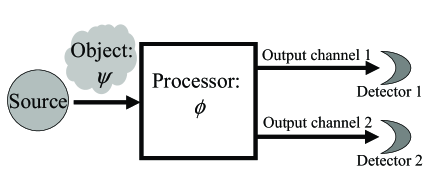
Consider the schematic representation of an experiment in which a source emits objects that carry information represented by an angle $0\leq\psi\leq 2\pi$ (see Fig. 1). We want to determine this angle as accurately as possible, but there are some limitations on the equipment that is available to us, namely:

Figure 1: Schematic representation of the event-by-event experiment. The source emits objects one at a time. Each object carries a message represented by an angle $\psi$. The processor combines this message with the angle $\phi$ that is controlled by the user, and sends the object through one of its two output channels. Detectors count the number of objects in each channel.

• We do not have a device that can measure the angle $\psi$ directly.

• We have detectors that can count the arrival (or passage) of individual objects.

• We can build a device, called processor in what follows, that can direct an incoming object to one of its two output channels according to $\psi$, relative to the orientation $0\leq\phi\leq 2\pi$ of the processor itself. We can count the number of objects in each output channel by using the detectors.

• We do not have prior information about the angle $\psi$ itself, implying that there is no reason to assume that particular angles $\psi$ are more likely to occur than others. Note that this does not imply that $\psi$ is a random variable.

Given this scenario, the obvious question is: What kind of functionality should we build into the processor such that by counting $N$ events in the output channels, we obtain an accurate estimate for the angle $\psi$ ? Of course, the optimal design of the processor depends on additional constraints. Usually, we prefer devices of which the output does not change drastically when the input varies a little. Therefore we require that

1. The number of events generated in each output channel is most insensitive to small changes in $\theta\equiv\psi-\phi$.

2. The performance of the processor should be insensitive to the actual value of $\theta$.

Using these two criteria, we consider two extreme realizations of the processor. First, we construct a simple probabilistic processor that operates according to the rules of probability theory and uses random numbers to transform the input data $\psi$ into a sequence of discrete output events. Then, we present a strictly deterministic processor that performs the same task as the simple probabilistic processor. In both cases, the general strategy to determine the optimal processor is the same: We search for a probabilistic or deterministic process that satisfies the criteria (1) and (2) mentioned earlier. Then we estimate the efficiency of the processor. As convenient measure for the efficiency (or performance) of a processor, we take the number of different messages $M_{D}$ that can be extracted from a record of $N$ bits, each bit representing an event in one of the two output channels, with a specified level of certainty.

The reader may have noticed that the scenario we described earlier applies to the measurement of the polarization of light in the regime where the signal from the detectors consists of discrete “clicks” BAYM74 ; FEYN65 . In this case, the objects are represented by photons, the angle $\psi$ describes the polarization (which we cannot measure directly), the detectors may be photon multiplier tubes or semiconductor diodes, and the processor a properly prepared calcite crystal BORN64 . In general terms, we want to characterize the behavior of a system in terms of numerical quantities that we can obtain by repeating measurements that give us partial information only. This is a characteristic feature of quantum mechanics. In order not to become entangled in the difficulties with the interpretation of quantum theory and the measurement paradox in particular HOME97 , in the theoretical analysis presented in this paper, we avoid the use of words such as photons and polarization. A remarkable result of this paper is that the search for an efficient (in the sense specified earlier), data processor yields probabilistic and deterministic processors that generate output events according to Malus’ law.

II Probabilistic processor

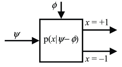
The schematic diagram of the probabilistic processor is shown in Fig. 2. The input to the processor is an event that carries a message represented by the angle $\psi$. The presence of an event in one of the output channels is represented by a message that carries the variable $x=\pm 1$. We assume that the experimental data is in concert with the hypothesis of rotational invariance. That is, the number of events in the $x=+1$ and $x=-1$ channels only depend on the difference $\theta=\psi-\phi$ between the (unknown) angle $\psi$ and the orientation of the device $0\leq\phi\leq 2\pi$. Furthermore, the number of output events should be periodic in $\theta$ with a period of $\pi$ known .

Let the probability $p(x|\theta)$ describe the process that transforms each input event into an output event $x=\pm 1$. By symmetry we have $p(x|\theta)=p(x|\theta+\pi)$ and if we assume that each input event generates exactly one output event we have

$$\sum_{x=\pm 1}p(x|\theta)=p(+1|\theta)+p(-1|\theta)=1.$$ (1)

We also assume that there is no logical dependence between two output events $i$ and $j$, that is $p(x_{i},x_{j}|\theta)=p(x_{i}|\theta)p(x_{j}|\theta)$ for all $i\not=j$. This implies that the correlation between the output events is zero. Then, this process generates Bernoulli trials GRIM95 ; TRIB69 ; JAYN03 .

Under these conditions, all information about the polarization is encoded in the measurable quantity

$$f(\theta)=\langle x\rangle=\sum_{x=\pm 1}xp(x|\theta)=2p(+1|\theta)-1.$$ (2)

From Eq. (2) it is clear that we can completely characterize the process by $p(\theta)\equiv p(+1|\theta)$.

Figure 2: Schematic diagram of a probabilistic processor that transforms the difference between the input angle $\psi$ and the setting $\phi$ into a sequence of $x=\pm 1$ signals.

Our task is to design the processor, that is to determine the function $p(\theta)$, such that a measurement of $f(\theta)$ gives us as much as possible knowledge about the unknown angle $\psi$.

Let us consider the data as collected by an observer who decides to record and analyze data sets of $N$ objects each. We assume that $\theta$ is fixed during this measurement. Each data set looks like $\{x_{1},\ldots,x_{N}\}$ where $x_{i}=\pm 1$ for $i=1,\ldots,N$. Let us assume that the number of $x_{i}=+1$ events in a particular data set is $n$. Recall that the processor generates Bernoulli trials TRIB69 ; GRIM95 ; JAYN03 . Therefore, the probability for observing this data set is given by TRIB69 ; GRIM95 ; JAYN03

$$P(n|\theta,N)=\frac{N!}{n!(N-n)!}p^{n}(\theta)[1-p(\theta)]^{N-n}.$$ (3)

For convenience of the reader, we first recall some well known facts of probability theory TRIB69 ; GRIM95 ; JAYN03 . From Eq.(3) it follows that, as a function of $p(\theta)$, $P(n|\theta,N)$ reaches its maximum $\hat{P}(n|\theta,N)$ at $\hat{p}(\theta)\equiv n/N$. A simple calculation shows that

$$\frac{1}{N}\ln\frac{P(n|\theta,N)}{\hat{P}(n|\theta,N)}=\hat{p}(\theta)\ln\frac{p(\theta)}{\hat{p}(\theta)}+(1-\hat{p}(\theta))\ln\frac{1-p(\theta)}{1-\hat{p}(\theta)}.$$ (4)

For small values of $|p(\theta)-\hat{p}(\theta)|$, the Taylor series expansion of the left hand side of Eq.(4) yields

$$\frac{P(n|\theta,N)}{\hat{P}(n|\theta,N)} = \exp\left[-N\frac{(p(\theta)-\hat{p}(\theta))^{2}}{2\hat{p}(\theta)(1-\hat{p}(\theta))}\right]$$ (5)

$$+ \hbox{${\cal O}((p(\theta)-\hat{p}(\theta))^{4})$},$$

showing that as a function of $p(\theta)$, $P(n|\theta,N)$ vanishes exponentially fast with $N$, unless $p(\theta)=\hat{p}(\theta)=n/N$ TRIB69 ; GRIM95 . Therefore, from the point of view of the observer, the procedure is simple: As the observer knows (the yet unknown) function $p(\theta)$, after measuring a data set $\{x_{1},\ldots,x_{N}\}$, the observer finds $\theta$ by solving $p(\theta)=n/N=\left(1+N^{-1}\sum_{i=1}^{N}x_{i}\right)/2$. The total number $n$ of $x_{i}=+1$ events contains all the available information about the difference $\theta=\psi-\phi$.

A rough estimate for the number of distinguishable messages $M_{D}$ that the probabilistic processor can encode with an error of approximately one percent can be obtained as follows. First, we use Eq. (3) to calculate the variance on $n$ and find that $\sigma^{2}(\theta)=N\hat{p}(\theta)(1-\hat{p}(\theta))$. For sufficiently large but fixed $N$, the probability distribution Eq. (3) tends to the normal (Gaussian) distribution with mean $n=Np(\theta)$ and variance $\sigma(\theta)$. Therefore, the probability to observe $m$ ($1\ll m\ll N$) instead of $n$ ($1\ll n\ll N$) $x_{i}=+1$ events is approximately given by

$$P(m|\theta,N) \approx \frac{1}{\sqrt{2\pi\sigma^{2}(\theta)}}\exp\left[-\frac{(m-n))^{2}}{2\sigma^{2}(\theta)}\right].$$ (6)

From the properties of the normal distribution, it follows that the probability for the observed number $m$ of $x_{i}=+1$ events to lie in the interval $[n-3\sigma(\theta),n+3\sigma(\theta)]$ is larger than $0.997$. Thus, the number of messages $M_{D}$ that can be encoded with a probability of error that is less that one percent is given by

$$M_{D} \approx N/6\sigma(\theta)\propto\sqrt{N}.$$ (7)

Although this is a rough estimate, the result that the number of distinguishable messages is of the order of $\sqrt{N}$ is to be expected on general grounds, given the constraint that the processor generates probabilistic, Bernoulli-like events.

We now apply the criteria 1 and 2 of Section I to optimize the design, that is we want to determine $p(\theta)$ by which the probabilistic (Bernoulli) processor will generate the output events. In the foregoing analysis, we assumed that $\theta$ was fixed during the observation of $N$ events. Clearly, this is not a realistic assumption. In a real experiment, $\phi$ or $\psi$ fluctuates. Therefore, the best we can do is search for the probability $p(\theta)$ that is least sensitive to small changes in $\phi-\psi$. This is criterion 1 of Section I.

We determine this probability by considering the likelihood that the observed sequence of $x_{i}$’s was generated by $p(x|\theta+\epsilon)$ instead of $p(x|\theta)$ where $\epsilon$ is a small positive number. The larger this likelihood, the larger the probability that the observer draws the wrong conclusion from the data. The log-likelihood $L$ that the data was generated by $p(x|\theta+\epsilon)$ instead of by $p(x|\theta)$ is given by TRIB69 ; JAYN03

$$\frac{L}{N} = \frac{1}{N}\ln\frac{P(n|\theta+\epsilon,N)}{P(n|\theta,N)},$$ (8)

$$= \frac{n}{N}\ln\frac{p(\theta+\epsilon)}{p(\theta)}+(1-\frac{n}{N})\ln\frac{1-p(\theta+\epsilon)}{1-p(\theta)}.$$

According to criterion 1 of Section I, we have to find the probability $p(\theta)$ that minimizes $|L|$.

We first consider the case that $P(n|\theta+\epsilon,N)>P(n|\theta,N)$. Then, because $P(n|\theta,N)$ is not the maximum, we assign $p(\theta+\epsilon)=n/N$ as the most likely guess. A Taylor series expansion of Eq. (8) yields

$$\ln\frac{P(n|\theta+\epsilon,N)}{P(n|\theta,N)}=\frac{\epsilon^{2}}{2p(\theta)(1-p(\theta))}\left(\frac{\partial p(\theta)}{\partial\theta}\right)^{2}.$$ (9)

Second, we consider the case that $P(n|\theta+\epsilon,N)\leq P(n|\theta,N)$. Now, adopting the same reasoning as used previously, the observer assigns $p(\theta)=n/N$ and the Taylor series expansion of Eq. (8) yields

$$\ln\frac{P(n|\theta+\epsilon,N)}{P(n|\theta,N)}=-\frac{\epsilon^{2}}{2p(\theta)(1-p(\theta))}\left(\frac{\partial p(\theta)}{\partial\theta}\right)^{2}.$$ (10)

As $\epsilon$ was arbitrary (but small), minimization of $|L|$ is equivalent to minimizing the Fisher information TREE68 ; FRIE99 ; BLAH91

$$I_{F}=\frac{1}{p(\theta)(1-p(\theta))}\left(\frac{\partial p(\theta)}{\partial\theta}\right)^{2},$$ (11)

for this particular problem. Thus, we conclude that the first criterion tells us that we should minimize the Fisher information $I_{F}$. Substituting $p(\theta)=\cos^{2}g(\theta)$ we obtain

$$I_{F}=4\left[\frac{\partial g(\theta)}{\partial\theta}\right]^{2}.$$ (12)

Criterion 2 of Section I stipulates that the reliability of the procedure to extract $\psi-\phi$ from the observed sequence of $x_{i}$’s should not depend on $\psi-\phi$. We can realize this by choosing $g(\theta)=a\theta+b$. Using the side information that $p(+1|\theta)=p(+1|\theta+\pi)$ we find that $p(+1|\theta)=\cos^{2}(k\theta+b)$ and $I_{F}=4k^{2}$ for $k\not=0$ ($k=0$ is excluded because then $p(\theta)$ does not depend on $\theta$ and the design leads to a useless device). Clearly $I_{F}$ is minimal if $k=1$ and we may absorb the irrelevant phase factor $b$ in $\phi$.

In summary, using the two design criteria of Section I, we find that for optimal operation (from the point of view of the observer), the processor should use the probabilities

$$p(-1|\theta)=\sin^{2}\theta\quad,\quad p(+1|\theta)=\cos^{2}\theta,$$ (13)

to generate the $-1$ and $+1$ events, respectively. Put differently, for a fixed processor setting $\phi$ and $N$ incoming events with message $\psi$, the observer will (in general) get most out of the data if the processor sends $N\cos^{2}(\psi-\phi)$ ($N\sin^{2}(\psi-\phi)$) events to the apparatus that detects the $+1$ ($-1$) event. The maximum number $M_{D}$ of angles $\psi-\phi$ we can distinguish is given by

$$M_{D}=a\sqrt{N},$$ (14)

where $a$ depends on the number of mistakes in determining $\psi-\phi$ that we find acceptable. The larger $a$, the larger is the probability that the result for $\psi-\phi$ is erroneous.

Obviously, it is easy to simulate this processor on a computer. For each of the $i=1,\ldots,N$ input events, we generate a uniform random number $0<r<1$ and send out a $x_{i}=+1$ ($x_{i}=-1$) event if $\cos^{2}\theta\leq r$ ($\cos^{2}\theta>r$). After processing $N$ events, we compute $\theta=\psi-\phi$ from $\cos^{2}\theta=\left(1+N^{-1}\sum_{i=1}^{N}x_{i}\right)/2$.

II.1 Relation to physics

Up to this point, there is no relation between the mathematical model that we have analyzed and a physical system. However, from the description of the scenario and the final result Eq. (13), it is obvious that a processor that operates according to Eq. (13) is a model for an ideal polarizer. We now discuss the relation between the optimal probabilistic processor and the measurement of the polarization of photons in more detail.

In classical electrodynamics, it is well known that the intensity of light transmitted by a polarizer (such as Nicol prism) is given by Malus’ law

$$I_{o}=I\sin^{2}(\psi-\phi)\quad,\quad I_{e}=I\cos^{2}(\psi-\phi),$$ (15)

where $I$, $I_{o}$, and $I_{e}$ are the intensities of the incident light, the ordinary and extraordinary ray, respectively, $\psi$ is the polarization of the incident light and $\phi$ specifies the orientation of the polarizer BORN64 . From a quantum mechanical point of view, the total energy $E$ of a light wave of frequency $f$ must be an integer multiple of $h$ (Planck’s constant), that is $E=nhf$, where $n$ is the number of photons in the wave. The polarizer splits the incoming beam in two beams. Depending on the type of polarizer, the light in one of the beams is absorbed BORN64 but this is irrelevant for the discussion that follows. In any case, the number of photons in each beam is an integer (by definition of the concept of a photon, there is no such thing as a half photon). If the number of photons in the incident beam is very large, the mean number of photons that goes into each beam should correspond to the intensity that we find from classical electrodynamics. In the regime where the photons are detected one-by-one, quantum mechanics postulates that the polarizer sends a photon to the (extra)ordinary direction with probability ($\sin^{2}(\psi-\phi)$) $\cos^{2}(\psi-\phi)$ BAYM74 .

The probabilistic processor that we have described transforms a beam of photons into yes/no events that we can count. If we require the answers of the transformation process to be probabilistic (Bernoulli trials), rotational invariant (a basic property of (quantum) electrodynamics), and to satisfy criteria 1 and 2 of Section I, then the device that performs the transformation will produce data that agrees with Malus’ law. We did not invoke any law of physics to obtain this result: Malus’ law was recovered as the result of efficient data processing. This raises the interesting question whether other quantum phenomena also appear as the result of efficient data processing.

The hypothesis that efficient processing of statistical information may be the reason why we observe quantum mechanical phenomena is very explicit in the work of Frieden FRIE99 , Wootters WOOT81 , and Summhammer SUMM01 . Frieden has shown that one can recover all the fundamental equations of physics by finding the extrema of the Fisher information plus the “bound” information FRIE99 . According to Frieden, the act of measurement elicits a physical law and quantum mechanics appears as the result of what Frienden calls ”a smart measurement”, a measurement that tries to make the best estimate FRIE99 . Although this approach is similar to ours, our line of reasoning is different. We do not invoke concepts from estimation theory, such as the estimators and the Cramér-Rao inequality (see Appendix A), nor do we require the concept of random noise. Furthermore, in Frieden’s formulation, the parameters to be estimated (such as the position) are of the same kind as the measured quantities. This is not the case for the photon polarization that we treat here. In our approach, the measuring apparatus (such as the calcite crystal acting as a polarizer) transforms the input (the photon polarization) into a signal ($x=\pm 1$) that can be detected by human beings. The requirement that the simple probabilistic processor, that transforms the data, operates with optimal efficiency yields Malus’ law.

The fundamental difference between Frienden’s approach and ours becomes evident by noting that there is no reason why we should limit our search for efficient transformation devices to the most simple, Bernoulli-type probabilistic machines. As we explain later, these machines can simulate the classical and quantum properties of a photon polarizer but are incapable of simulating interference phenomena. One possible route to solve this problem might be to generalize the probabilistic machine such that it no longer generates Bernoulli events, that is allow for correlations between output events. We don’t follow this route. Instead we consider the most extreme solution, namely a deterministic processor that performs the same task as the probabilistic machine under the conditions specified in Section I. This forces us to consider deterministic algorithms with primitive learning capabilities (to allow for correlations between output events). Elsewhere, we have shown that these deterministic processors (and probabilistic versions thereof) can be used to reproduce quantum interference phenomena KRAED05 ; HRAED05a ; MICH05 ; HRAED05b . We come back to this topic in Section IV.

III Deterministic processor

From an engineering point of view, the probabilistic processor of Section II is extremely simple and has a relatively poor performance. Using $N$ bits, the probabilistic processor can encode $M_{D}\propto\sqrt{N}$ distinguishable messages only. For example, as shown in Section II, if we demand the level of certainty of 99.7%, then $M_{D}\approx\sqrt{N}/6$.

It is not unreasonable to expect that a deterministic machine can do better in this respect. Therefore, the obvious question is to ask if there exists a deterministic processor that generates events according to Malus’ law. Apart from being deterministic, this processor should satisfy the two criteria that we specified in Section I.

Adopting the terminology introduced in our earlier work KRAED05 ; HRAED05a ; MICH05 ; HRAED05b , we refer to the deterministic processor that we describe in this section as a deterministic learning machine (DLM). For this machine, $M_{D}=N+1$ with nearly 100% certainty.

In this paper, we analyze a DLM that has one input channel, two output channels and one internal vector with two real entries. A DLM responds to an input event by choosing from all possible alternatives, the internal state that minimizes a cost function (to be defined later) that depends on the input and the internal state itself. Then the DLM sends a message through one of its output channels. The message contains information about the decision the DLM took while it updated its internal state and, depending on the application, also contains other data that the DLM may have. By updating its internal state, the DLM “learns” about the input it receives and by sending messages through one of its two output channels, it tells its environment about what it has learned. A DLM is a machine that performs real-time recurrent learning HAYK99 .

This section consists of three parts. First, we specify the algorithm that is used by a DLM and we show that in the stationary regime, the number of $-1$ ($+1$) events in a sequence of $N$ events is given by Malus’ law, see Eq. (15). Then, we present a detailed mathematical analysis of the dynamic properties of a DLM. The reader who is not interested in the intricacies of this classical dynamical system can skip Section III.2. We end this section by comparing the performance of the probabilistic and deterministic processor.

III.1 Deterministic Learning Machines

The schematic diagram of the DLM is the same as that of the probabilistic processor of Fig. 2, except that there is no probabilistic process $p(x|\psi-\phi)$. The DLM receives as input, a sequence of angles $\psi_{n+1}$ for $n=0,\ldots,N$ and also knows about the orientation of the device through the angle $\phi$. Using rotational invariance, we represent these input messages by unit vectors ${\bf y}_{n+1}=(y_{1,n+1},y_{2,n+1})$ where

$$y_{1,n+1}=\cos\theta_{n+1}\quad y_{2,n+1}=\sin\theta_{n+1},$$ (16)

and $\theta_{n}=\psi_{n}-\phi$. The fact that Eq. (16) depends on the relative difference of the angles guarantees that the deterministic process is rotational invariant. Instead of the random number generator that is part of the probabilistic processor, the DLM has an internal degree of freedom that we represent by the unit vector ${\bf x}_{n+1}=(x_{1,n+1},x_{2,n+1})$. As the DLM receives input data, it updates its internal state. For all $n>0$, the update rules are defined by

$$x_{1,n+1} = \alpha x_{1,n}+\beta(1-\Theta_{n+1}),$$

$$x_{2,n+1} = \alpha x_{2,n}+\beta\Theta_{n+1},$$ (17)

where $\Theta_{n+1}=0$ ($1$) corresponds to an $-1$ ($+1$) output event, and $0<\alpha<1$ is a parameter that controls the learning process of the DLM. The requirement that the internal vector ${\bf x}_{n+1}=(x_{1,n+1},x_{2,n+1})$ stays on the unit circle yields

$$\beta= \pm \sqrt{1+\alpha^{2}[x_{1,n}^{2}(1-\Theta_{n+1})+x_{2,n}^{2}\Theta_{n+1}-1]}$$ (18)

$$- \alpha[x_{1,n}(1-\Theta_{n+1})+x_{2,n}\Theta_{n+1}].$$

Substitution of Eq. (18) in Eq. (17) gives us four different rules:

$$x_{1,n+1}= +\sqrt{1+\alpha^{2}(x_{1,n}^{2}-1)},\quad x_{2,n+1}=\alpha x_{2,n},$$

$$x_{1,n+1}= -\sqrt{1+\alpha^{2}(x_{1,n}^{2}-1)},\quad x_{2,n+1}=\alpha x_{2,n},$$

$$x_{1,n+1}= \alpha x_{1,n},\quad x_{2,n+1}=+\sqrt{1+\alpha^{2}(x_{2,n}^{2}-1)},$$

$$x_{1,n+1}= \alpha x_{1,n},\quad x_{2,n+1}=-\sqrt{1+\alpha^{2}(x_{2,n}^{2}-1)},$$ (19)

where the first (last) two rules correspond to the choice $\Theta_{n+1}=0$ ($\Theta_{n+1}=1$) and the $\pm$-sign takes care of the fact that for each choice of $\Theta_{n+1}$, the DLM has to decide between two quadrants. For later, it is important to note that $|x_{1,n+1}|>|x_{1,n}|$ and $|x_{2,n+1}|<|x_{2,n}|$ if $\Theta_{n+1}=0$. In other words, the angle of the internal vector relative to the $x$-axis decreases if we apply the $\Theta_{n+1}=0$ rules. The DLM selects one of the four rules in Eq. (19) by minimizing the cost function defined by

$$C = -{\bf x}_{n+1}\cdot{\bf y}_{n+1}=({\bf x}_{n+1}-{\bf y}_{n+1})^{2}/2-1$$ (20)

$$= -(x_{1,n+1}y_{1,n+1}+x_{2,n+1}y_{2,n+1}).$$

Obviously, the cost $C$ is small if the vectors ${\bf x}_{n+1}$ and ${\bf y}_{n+1}$ are close to each other. Summarizing: a DLM minimizes the distance between the input vector and its internal vector by means of a simple, deterministic decision process.

Figure 3: (color online) Time evolution of the angle $\theta_{n}=\arctan(x_{2,n}/x_{1,n})$ representing the internal vector ${\bf x}_{n}$ of the DLM defined by Eqs. (19) and (20). Bullets (red): Input events carry vectors ${\bf y}_{n+1}=(\cos 60^{\circ},\sin 60^{\circ})$. The initial value $\theta_{0}\approx 81^{\circ}$. For $n>20$ the ratio of the number of increments ($\Theta_{n+1}=1$) to decrements ($\Theta_{n+1}=0$) is exactly 3/1, which is $(\sin 60^{\circ}/\cos 60^{\circ})^{2}$. Squares (blue): Input events carry vectors ${\bf y}_{n+1}=(\cos 30^{\circ},\sin 30^{\circ})$. The initial value $\theta_{0}\approx 327^{\circ}$. For $n>60$ the ratio of the number of increments ($\Theta_{n+1}=1$) to decrements ($\Theta_{n+1}=0$) is exactly 1/3, which is $(\sin 30^{\circ}/\cos 30^{\circ})^{2}$. The direction of the initial vectors ${\bf x}_{0}$ is chosen at random. In this simulation $\alpha=0.99$. Data for $n<10$ has been omitted to show the oscillating behavior more clearly. Lines are guides to the eyes.

Figure 4: The number of ($\Theta_{n+1}=1$) events divided by the total number of events as a function of the value of the input variable $\theta$. Bullets: Each data point is obtained from a DLM simulation of 1000 events with a fixed, randomly chosen value of $0\leq\phi<360^{\circ}$, using the last 500 events to count the number of ($\Theta_{n+1}=1$) events. Solid line: $\cos^{2}\theta$.

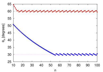
In general, the behavior of the DLM defined by rules Eqs. (19) and (20) is difficult to analyze without the use of a computer. However, for a fixed input vector ${\bf y}_{n+1}={\bf y}$, it is clear what the DLM will try to do: It will minimize the cost Eq. (20) by rotating its internal vector ${\bf x}_{n+1}$ to bring it as close as possible to ${\bf y}$. However, ${\bf x}_{n+1}$ will not converge to a limiting value but instead it will keep oscillating about the input value ${\bf y}$. An example of a simulation is given in Fig. 3. In general, for a fixed input vector ${\bf y}_{n+1}={\bf y}$ the DLM will reach a state in which its internal vector oscillates about ${\bf y}$. This is the stationary state of the machine. Obviously, the whole process is deterministic. The details of the approach to the stationary state depend on the initial value of the internal vector ${\bf x}_{0}$, but the properties of the stationary state do not.

III.1.1 Stationary state

The stationary-state analysis is a very useful tool to understand the behavior of the DLMs. Let us assume that $0\ll\alpha<1$ and that we have reached the stationary regime in which the internal vector performs small oscillations about $(\cos\theta,\sin\theta)$ (as in Fig. 3). For simplicity, but without loss of generality, we limit the discussion that follows to $0\leq\theta\leq\pi/2$. For $\Theta_{n+1}=0$ we substitute $x_{2,n}=\sin\varphi_{n}$ and $\theta_{n+1}=\varphi_{n}+\delta_{0}$ in Eq. (19) and obtain

$$\sin^{2}\varphi_{n}+2\delta_{0}\sin\varphi_{n}\cos\varphi_{n} = \alpha^{2}\sin^{2}\varphi_{n}.$$ (21)

Similarly, for $\Theta_{n+1}=1$ we substitute $x_{2,n}=\sin\varphi_{n}$ and $\theta_{n+1}=\varphi_{n}+\delta_{1}$ in Eq. (19) and obtain

$$\sin^{2}\varphi_{n}+2\delta_{1}\sin\varphi_{n}\cos\varphi_{n} = -\alpha^{2}\cos^{2}\varphi_{n}+1.$$ (22)

In deriving Eqs. (21) and  (22), we neglected terms of order $\delta^{2}_{0}$ and $\delta^{2}_{1}$, respectively. Rearranging Eqs. (21) and  (22), and using $\varphi_{n}\approx\theta$ gives

$$\delta_{0} = -\frac{1-\alpha^{2}}{2}\frac{\sin\theta}{\cos\theta}\quad\hbox{if\ \ }\Theta_{n+1}=0,$$

$$\delta_{1} = \phantom{-}\frac{1-\alpha^{2}}{2}\frac{\cos\theta}{\sin\theta}\quad\hbox{if\ \ }\Theta_{n+1}=1.$$ (23)

In the stationary regime, the sum of all increments of $\varphi_{n}$ should be compensated by the sum of all decrements of $\varphi_{n}$. Therefore, we must have $N_{0}\delta_{0}+N_{1}\delta_{1}\approx 0$ where $N_{0}$ ($N_{1}$) is the number of $\Theta_{n+1}=0$ ($\Theta_{n+1}=1$) events. From Eq. (23) it follows immediately that

$$\tan^{2}\theta\approx\frac{N_{1}}{N_{0}},$$ (24)

and hence

$$\frac{N_{1}}{N_{0}+N_{1}}\approx\sin^{2}\theta\quad,\quad\frac{N_{0}}{N_{0}+N_{1}}\approx\cos^{2}\theta.$$ (25)

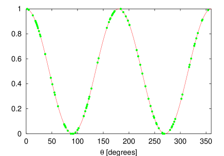
Fig. 4 shows that the simulation results generated by the DLM are in excellent agreement with the expressions obtained from this simple analysis. In fact, we will see later that in the stationary state, a DLM can encode exactly all angles for which $\sin^{2}\theta=n/N$ where $n=0,\ldots,N$. From the definition of the DLM algorithm and Eq. (25), it is clear that the requirements of rotational invariance and insensitivity with respect to small changes in $\theta=\phi-\psi$ (criterion 1 of Section I) are automatically satisfied. We emphasize that Eq. (25) is not put into the DLM algorithm but results from the learning process itself.

Comparing Eq. (15) and Eq. (25), we conclude that once the DLM has reached a stationary state, the number of $+1$ and $-1$ output events in a sequence of $N=N_{0}+N_{1}$ events agrees with Malus’ law. Of course, the order in which the DLM generates the $+1$ and $-1$ is strictly deterministic. Anticipating that we will show that a DLM is a very efficient machine, what is most striking is that the number of $-1$ and $+1$ events it generates is proportional to $\sin^{2}(\psi-\phi)$ and $\cos^{2}(\psi-\phi)$, respectively, just as in the case of the simple probabilistic processor and in the classical electrodynamical and quantum mechanical description of the polarizer.

III.2 Analysis of the dynamic properties

For a more detailed mathematical analysis of the dynamics of a DLM, it is convenient to write the update rules Eq. (19) as linear difference equations. Actually, we need only

$$x_{2,n+1}^{2} = \alpha^{2}x_{2,n}^{2}+(1-\alpha^{2})\Theta_{n+1}.$$ (26)

For simplicity, we restrict the discussion that follows to the case $0\leq\theta\leq\pi/4$. Other cases can be treated in the same manner.

Substituting $x_{2,n}=\sin\varphi_{n}$ in Eq. (26), we obtain

$$\sin^{2}\varphi_{n+1} = \alpha^{2}\sin^{2}\varphi_{n}+(1-\alpha^{2})\Theta_{n+1},$$ (27)

showing that Eq. (26) has the structure of a so-called circle map JENS83 . Thus, the study of the behavior of the circle map Eq. (27) will give us insight into the dynamic properties of the DLM. Fig. 5 shows an example of circle-map analysis for the case of a fixed input angle of $30^{\circ}$.

Figure 5: (color online) Circle map of the time evolution of $x^{2}_{2,n}$ for the case of a fixed input angle of $30^{\circ}$. The dashed (green) line shows the evolution of the mapping $x^{2}_{2,n+1}=F(x^{2}_{2,n})$ for $n<100$. For clarity, we omitted the first 12 iterations because this allows us to show in detail how the mapping converges to a unique polygon. The function $F(x^{2})$ is defined by the rules and cost function Eq. (19) and Eq. (20), respectively. The dotted (blue) line separates the case $\Theta_{n+1}=0$ from the case $\Theta_{n+1}=1$ and is given by $y=\alpha^{2}x+1-\alpha^{2}$ for $\Theta_{n+1}=1$ ($x<1/4$) and $y=\alpha^{2}x$ for $\Theta_{n+1}=0$ ($x>1/4$). The straight solid (red) line is given by $y=x$. The solid (red) line forming the polygon with eight vertices shows the results for $9900\leq n<10000$: In this case the system has reached the stationary state with a period of four. In this simulation, $\alpha=0.99$.

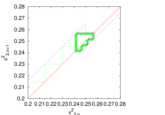
III.2.1 Illustrative example

Let us assume that we have reached a stationary state and that the DLM repeats a sequence $\{00\ldots 00100\ldots 00100\ldots\}$ in which there are $K$ successive events of the type $\Theta_{n+1}=0$ (decreasing $x_{2,j}$) and one $\Theta_{n+1}=1$ event (increasing $x_{2,j}$). Let us denote by $\hat{x}$, the value of $x_{2,n+1}$ before the first of the $K$ events of type 0. From Eq. (26) we obtain

$$x_{2,K}^{2} = \alpha^{2K}\hat{x}^{2},$$

$$x_{2,K+1}^{2} = \alpha^{2}x_{2,K}^{2}+1-\alpha^{2},$$ (28)

$$= \alpha^{2K+2}\hat{x}^{2}+1-\alpha^{2}$$

As the DLM repeats the same sequence over and over again, we have $x_{2,K+1}^{2}=\hat{x}^{2}$. In other words, if we observe the repeated sequence $\{00\ldots 01\}$ of length $K+1$, we must have

$$\hat{x}^{2} = \frac{1-\alpha^{2}}{1-\alpha^{2K+2}}.$$ (29)

Furthermore, as $x_{2,j}^{2}=\alpha^{2j}\hat{x}^{2}$ for $j=0,\ldots,K$, the mean value of the $x^{2}_{2,j}$’s during the sequence is given by

$$\langle x^{2}\rangle \equiv \frac{1}{K+1}\sum_{j=0}^{K}x_{2,j}^{2}=\frac{1}{K+1}\approx\sin^{2}\theta,$$ (30)

in agreement with Eq. (25). From Eq. (30), we conclude that the DLM can encode the values $\theta=\arctan(1/\sqrt{K})$ with periodic sequences of the form $\{00\ldots 01\}$.

From this analysis we conclude that if we would limit the design of the device such that it can only generate sequences of the form $\{00\ldots 01\}$, then, after observing two one’s and counting the zeros between these two one’s, we can determine the angle with an error of less than 5 degrees. This is the worst case and occurs when the sequence is $\{010101010\ldots\}$ ($45\deg$) and $\{0010010010\ldots\}$ ($35\deg$). Clearly, even with this limitation ($K$ zero’s followed by one $1$) on the design, this is already a very efficient method to encode the angle.

We now extend this analysis to a general periodic sequence.

III.2.2 Minimum angle

First we show how the control parameter $\alpha$ limits the accuracy with which we can represent the stationary state. Let us assume that the fixed input vector is given by ${\bf y}=(y_{1},y_{2})$ and that for some index $n$, the machine is in the state ${\bf x}_{n}=(1,0)$, as illustrated in Fig. 6 (the cases $(0,1)$, $(-1,0)$, and $(0,-1)$ can be treated in the same manner and lead to the same conclusion).

If the machine applies the update rule $\Theta_{n+1}=0$, the new state and the cost are given by

$$x_{1,n+1} = \sqrt{1+\alpha^{2}(x_{1,n}^{2}-1)}=1,$$

$$x_{2,n+1} = \alpha x_{2,n}=0,$$

$$C = -y_{1}.$$ (31)

The cost $C$ has to be compared to the cost of applying the update rule $\Theta_{n+1}=1$, in which case we have

$$x_{1,n+1} = \alpha x_{1,n}=\alpha,$$

$$x_{2,n+1} = \sqrt{1+\alpha^{2}(x_{2,n}^{2}-1)}=\sqrt{1-\alpha^{2}},$$

$$C = -(\alpha y_{1}+y_{2}\sqrt{1-\alpha^{2}}).$$ (32)

Figure 6: (color online) Illustration of a situation in which the machine remains in the state ${\bf x}=(1,0)$. The input vector is ${\bf y}=(y_{1},y_{2})$. The internal state is ${\bf x}_{n}=(1,0)$, and the new internal state is either ${\bf x}_{n+1}=(\alpha,\sqrt{1-\alpha^{2}})$ or ${\bf x}_{n+1}=(1,0)$. In general, the smallest angle $\theta_{min}$ for which the machine remains in the state ${\bf x}=(1,0)$ depends on the value of the parameter $\alpha$, see Eq. (35).

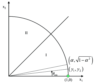
Note that the point $(1,0)$ is somewhat special in the sense that the machine remains at $(1,0)$ if it applies the update rule $\Theta_{n+1}=0$. The machine stays at $(1,0)$ (forever) unless the cost of applying the update rule $\Theta_{n+1}=1$, is less than the cost of applying the update rule $\Theta_{n+1}=0$. From Eqs. (31) and (32), the necessary condition for the machine not to get stuck at $(1,0)$ is

$$\alpha y_{1}+y_{2}\sqrt{1-\alpha^{2}}>y_{1}.$$ (33)

Rearranging Eq. (33) yields

$$\tan^{2}\theta=\frac{y_{2}^{2}}{y_{1}^{2}}>\frac{1-\alpha}{1+\alpha}.$$ (34)

Thus, Eq. (32) shows that we cannot represent angles $\theta$ that are smaller than

$$\theta_{min} = \arctan\sqrt{(1-\alpha)/(1+\alpha)}.$$ (35)

For $\alpha=0.99$ ($0.999$), typical values used in simulations, $\theta_{min}=4.05^{\circ}$ ($1.28^{\circ}$). Note that $\theta_{min}$ does not determine the accuracy in the interval $[\theta_{min},\pi/4]$.

III.2.3 Periodic sequences: General case

We now consider situations in which the sequence of events consists of a repetition of the sequence $\{\Theta_{n+1},\Theta_{n+2},\ldots,\Theta_{n+N};\Theta_{n}=\Theta_{n+N}\}$ of length $N$. First, we determine the solution $\hat{x}_{2,n}^{2}$ of $x_{2,n}^{2}=x_{2,n+N}^{2}$ (implying $x_{1,n}^{2}=x_{1,n+N}^{2}$). The formal solution of Eq. (26) is given by

$$x_{2,n+k}^{2} = \alpha^{2k}x_{2,n}^{2}+(1-\alpha^{2})\sum_{j=1}^{k}\alpha^{2(k-j)}\Theta_{n+j},$$ (36)

and the requirement $x_{2,n}^{2}=x_{2,n+N}^{2}$ yields

$${\hat{x}}_{2,n+N}^{2} = \frac{1-\alpha^{2}}{1-\alpha^{2N}}\sum_{j=1}^{N}\alpha^{2(N-j)}\Theta_{n+j}.$$ (37)

We conclude that if the machine starts from $\hat{x}_{2,n}^{2}$ and generates the events $\{\Theta_{n+1},\Theta_{n+2},\ldots,\Theta_{n+N}\}$, it returns to the starting point $\hat{x}_{2,n}^{2}$. For each pattern $\{\Theta_{n+1},\Theta_{n+2},\ldots,\Theta_{n+N}\}$, there exists such a point $\hat{x}_{2,n}^{2}$. In other words, if the machine is in the state $\hat{x}_{2,n}^{2}$, repeating the sequence $\{\Theta_{n+1},\Theta_{n+2},\ldots,\Theta_{n+N}\}$ generates a periodic motion of $x_{2,n+k}^{2}$ for $k>0$ with period $N$.

Second, we consider the situation in which the machine starts from $\hat{x}_{2,n}^{2}+\epsilon$ and we keep feeding the machine with the periodic sequence $\{\Theta_{n+1},\Theta_{n+2},\ldots,\Theta_{n+N}\}$. Using the general expression Eq. (36), we find

$$x_{2,n+pN}^{2} = \alpha^{2pN}\hat{x}_{2,n}^{2}+\alpha^{2pN}\epsilon$$ (38)

$$+(1-\alpha^{2})\sum_{j=1}^{pN}\alpha^{2(pN-j)}\Theta_{n+j},$$

$$= \alpha^{2N}\hat{x}_{2,n+(p-1)N}^{2}+\alpha^{2pN}\epsilon$$

$$+(1-\alpha^{2})\sum_{j=1}^{N}\alpha^{2(N-j)}\Theta_{n+j},$$

$$= \alpha^{2N}\hat{x}_{2,n}^{2}+\alpha^{2pN}\epsilon$$

$$+(1-\alpha^{2})\sum_{j=1}^{N}\alpha^{2(N-j)}\Theta_{n+j},$$

where $p$ denotes the number of times the machine processes the periodic sequence $\{\Theta_{n+1},\Theta_{n+2},\ldots,\Theta_{n+N}\}$. As $\alpha<1$, $\lim_{p\rightarrow\infty}x_{2,n+pN}^{2}=\hat{x}_{2,n}^{2}$, independent of the choice of $\epsilon$. Therefore, for any periodic sequence $\{\Theta_{n+1},\Theta_{n+2},\ldots,\Theta_{n+N};\Theta_{n}=\Theta_{n+N}\}$ of length $N$, the corresponding sequence $\{x_{2,j+1}^{2},x_{2,j+2}^{2},\ldots,x_{2,j+N}^{2}\}$ converges exponentially fast to the periodic sequence $\{\hat{x}_{2,j+1}^{2},\hat{x}_{2,j+2}^{2},\ldots,\hat{x}_{2,j+N}^{2}\}$. From Eq. (25) it then follows that

$$\frac{1}{N}\sum_{i=0}^{N-1}\hat{x}_{2,n+1+i}^{2} = \frac{\alpha^{2}}{N}\sum_{i=0}^{N-1}\hat{x}_{2,n+i}^{2}$$ (39)

$$+\frac{1-\alpha^{2}}{N}\sum_{i=0}^{N-1}\Theta_{n+1+i}.$$

and using $\hat{x}_{2,n+N}=\hat{x}_{2,n}$ we find

$$\frac{1}{N}\sum_{j=1}^{N}\hat{x}_{2,n+j}^{2} = \frac{1}{N}\sum_{j=1}^{N}\Theta_{n+j}\equiv{\bar{\Theta}}.$$ (40)

Note that ${\bar{\Theta}}$ is a rational number and that according to Eq. (25), we have ${\bar{\Theta}}\approx\sin^{2}\theta$.

III.2.4 Lowerbound on the control parameter $\alpha$

Previously, we have tactically assumed that we can always find the periodic sequence of $\Theta_{n}$’s that represents the input angle $\theta$. We now show that for a fixed input angle $\theta$, the control parameter $\alpha$ has to be large enough (but smaller than one) in order that the DLM repeats the same sequence $\{\Theta_{n+1},\Theta_{n+2},\ldots,\Theta_{n+N}\}$. As before, we confine the discussion to input angles that satisfy $0\leq\tan\theta=y_{2}/y_{1}\leq 1$. Then, the number of 0 events is larger than the number of 1 events. Without loss of generality, we may put $\Theta_{n+1}=0$. This means that the internal state $(x_{1,n},x_{2,n})$ of the DLM satisfies $x_{2,n}>y_{2}$. If the sequence is to be periodic with period $N$, we must have $x_{2,n+N}=x_{2,n}$.

Figure 7: Plot of the function $f(\alpha,K)$ (see Eq. (44)) as a function of $\alpha$ for $K=57$ (solid line) and $K=80$ (dashed line). In the stationary regime and for $f(\alpha,K)>0$, the DLM repeats the sequence $\{00\ldots 001\}$ with $K$ zero’s, that is, it generates and exact representation of $K$.

Table 1: Sequences $\{\Theta_{1},\ldots,\Theta_{q}\}$ marked with a ^∗ yield the smallest variance $\Delta^{2}$.

$\bar{\Theta}=p/q$	$\{\Theta_{1},\ldots,\Theta_{q}\}$	$\hat{x}_{2,0}^{2}$	$\Delta^{2}$
$1/2$	10∗	$\frac{\alpha^{2}}{{1+\alpha^{2}}}$	$\frac{{\left(1-\alpha^{2}\right)}^{2}}{4\,{\left(1+\alpha^{2}\right)}^{2}}$
$1/3$	100∗	$\frac{\alpha^{4}}{{{1+\alpha^{2}+\alpha^{4}}}}$	$\frac{2\,{\left(1-\alpha^{2}\right)}^{2}}{9\,\left(1+\alpha^{2}+\alpha^{4}\right)}$
$1/4$	1000∗	$\frac{\alpha^{6}}{(1+\alpha^{2})(1+\alpha^{4})}$	$\frac{{\left(1-\alpha^{2}\right)}^{2}\,\left(3+4\,\alpha^{2}+3\,\alpha^{4}\right)}{16\,{\left(1+\alpha^{2}\right)}^{2}\,\left(1+\alpha^{4}\right)}$
$2/5$	11000	$\alpha^{6}\,{{\frac{1-\alpha^{4}}{1-\alpha^{10}}}}$	$\frac{2\,{\left(1-\alpha^{2}\right)}^{2}\,\left(3+4\,\alpha^{2}+3\,\alpha^{4}\right)}{25\,\left(1+\alpha^{2}+\alpha^{4}+\alpha^{6}+\alpha^{8}\right)}$
$2/5$	10100∗	$\alpha^{8}\,{{\frac{(1+\alpha^{4})(1-\alpha^{2})}{1-\alpha^{10}}}}$	$\frac{2\,{\left(1-\alpha^{2}\right)}^{2}\,\left(3-\alpha^{2}+3\,\alpha^{4}\right)}{25\,\left(1+\alpha^{2}+\alpha^{4}+\alpha^{6}+\alpha^{8}\right)}$
$2/8$	11000000	$\alpha^{12}\,\frac{1-\alpha^{4}}{1-\alpha^{16}}$	$\frac{{\left(1-\alpha^{2}\right)}^{2}\,\left(3+2\,\alpha^{2}+4\,\alpha^{4}+2\,\alpha^{6}+3\,\alpha^{8}\right)}{16\,\left(1+\alpha^{4}+\alpha^{8}+\alpha^{12}\right)}$
$2/8$	10100000	$\alpha^{10}\,\frac{1}{{{1+\alpha^{2}+\alpha^{8}+\alpha^{10}}}}$	$\frac{{\left(1-\alpha^{2}\right)}^{2}\,\left(3+4\,\alpha^{2}+4\,\alpha^{4}+4\,\alpha^{6}+3\,\alpha^{8}\right)}{16\,{\left(1+\alpha^{2}\right)}^{2}\,\left(1+\alpha^{8}\right)}$
$2/8$	10010000	$\alpha^{8}\,{{\frac{1-\alpha^{2}+\alpha^{4}}{1+\alpha^{4}+\alpha^{8}+\alpha^{12}}}}$	$\frac{{\left(1-\alpha^{2}\right)}^{2}\,\left(3-2\,\alpha^{2}+4\,\alpha^{4}-2\,\alpha^{6}+3\,\alpha^{8}\right)}{16\,\left(1+\alpha^{4}+\alpha^{8}+\alpha^{12}\right)}$
$2/8$	10001000∗	$\alpha^{6}\,\frac{1-\alpha^{2}}{{{1-\alpha^{8}}}}$	$\frac{{\left(1-\alpha^{2}\right)}^{2}\,\left(3+4\,\alpha^{2}+3\,\alpha^{4}\right)}{16\,{\left(1+\alpha^{2}\right)}^{2}\,\left(1+\alpha^{4}\right)}$
$3/8$	11100000	$\alpha^{10}\,{{\frac{1-\alpha^{6}}{1-\alpha^{16}}}}$	$\frac{{\left(1-\alpha^{2}\right)}^{2}\,\left(15+44\,\alpha^{2}+71\,\alpha^{4}+80\,\alpha^{6}+71\,\alpha^{8}+44\,\alpha^{10}+15\,\alpha^{12}\right)}{64\,{\left(1+\alpha^{2}\right)}^{2}\,\left(1+\alpha^{4}+\alpha^{8}+\alpha^{12}\right)}$
$3/8$	10110000	$\alpha^{8}\,{{\frac{1-\alpha^{4}+\alpha^{6}-\alpha^{8}}{1-\alpha^{16}}}}$	$\frac{{\left(1-\alpha^{2}\right)}^{2}\,\left(15+28\,\alpha^{2}+39\,\alpha^{4}+48\,\alpha^{6}+39\,\alpha^{8}+28\,\alpha^{10}+15\,\alpha^{12}\right)}{64\,{\left(1+\alpha^{2}\right)}^{2}\,\left(1+\alpha^{4}+\alpha^{8}+\alpha^{12}\right)}$
$3/8$	10011000	$\alpha^{6}\,{{\frac{1-\alpha^{4}+\alpha^{8}-\alpha^{10}}{1-\alpha^{16}}}}$	$\frac{{\left(1-\alpha^{2}\right)}^{2}\,\left(15+28\,\alpha^{2}+23\,\alpha^{4}+16\,\alpha^{6}+23\,\alpha^{8}+28\,\alpha^{10}+15\,\alpha^{12}\right)}{64\,{\left(1+\alpha^{2}\right)}^{2}\,\left(1+\alpha^{4}+\alpha^{8}+\alpha^{12}\right)}$
$3/8$	11010000	$\alpha^{8}\,{{\frac{1-\alpha^{2}+\alpha^{4}-\alpha^{8}}{1-\alpha^{16}}}}$	$\frac{{\left(1-\alpha^{2}\right)}^{2}\,\left(15+28\,\alpha^{2}+39\,\alpha^{4}+48\,\alpha^{6}+39\,\alpha^{8}+28\,\alpha^{10}+15\,\alpha^{12}\right)}{64\,{\left(1+\alpha^{2}\right)}^{2}\,\left(1+\alpha^{4}+\alpha^{8}+\alpha^{12}\right)}$
$3/8$	10101000	$\alpha^{6}\,{{\frac{(1-\alpha^{2})(1+\alpha^{4}+\alpha^{8})}{1-\alpha^{16}}}}$	$\frac{{\left(1-\alpha^{2}\right)}^{2}\,\left(15+12\,\alpha^{2}+23\,\alpha^{4}+16\,\alpha^{6}+23\,\alpha^{8}+12\,\alpha^{10}+15\,\alpha^{12}\right)}{64\,{\left(1+\alpha^{2}\right)}^{2}\,\left(1+\alpha^{4}+\alpha^{8}+\alpha^{12}\right)}$
$3/8$	10010100∗	$\alpha^{4}\,{{\frac{(1-\alpha^{2})(1+\alpha^{4}+\alpha^{10})}{1-\alpha^{16}}}}$	$\frac{{\left(1-\alpha^{2}\right)}^{2}\,\left(15+12\,\alpha^{2}+7\,\alpha^{4}+16\,\alpha^{6}+7\,\alpha^{8}+12\,\alpha^{10}+15\,\alpha^{12}\right)}{64\,{\left(1+\alpha^{2}\right)}^{2}\,\left(1+\alpha^{4}+\alpha^{8}+\alpha^{12}\right)}$
$3/8$	11001000	$\alpha^{6}\,{{\frac{1-\alpha^{2}+\alpha^{6}-\alpha^{10}}{1-\alpha^{16}}}}$	$\frac{{\left(1-\alpha^{2}\right)}^{2}\,\left(15+28\,\alpha^{2}+23\,\alpha^{4}+16\,\alpha^{6}+23\,\alpha^{8}+28\,\alpha^{10}+15\,\alpha^{12}\right)}{64\,{\left(1+\alpha^{2}\right)}^{2}\,\left(1+\alpha^{4}+\alpha^{8}+\alpha^{12}\right)}$
$2/9$	110000000	$\alpha^{14}\,{{\frac{1-\alpha^{4}}{1-\alpha^{18}}}}$	$\frac{2\,{\left(1-\alpha^{2}\right)}^{2}\,\left(7+12\,\alpha^{2}+15\,\alpha^{4}+16\,\alpha^{6}+15\,\alpha^{8}+12\,\alpha^{10}+7\,\alpha^{12}\right)}{81\,\left(1+\alpha^{2}+\alpha^{4}\right)\,\left(1+\alpha^{6}+\alpha^{12}\right)}$
$2/9$	101000000	$\alpha^{12}\,{{\frac{1-\alpha^{2}+\alpha^{4}-\alpha^{6}}{1-\alpha^{18}}}}$	$\frac{2\,{\left(1-\alpha^{2}\right)}^{2}\,\left(7+3\,\alpha^{2}+15\,\alpha^{4}+7\,\alpha^{6}+15\,\alpha^{8}+3\,\alpha^{10}+7\,\alpha^{12}\right)}{81\,\left(1+\alpha^{2}+\alpha^{4}+\alpha^{6}+\alpha^{8}+\alpha^{10}+\alpha^{12}+\alpha^{14}+\alpha^{16}\right)}$
$2/9$	100100000	$\alpha^{10}\,{{\frac{1-\alpha^{2}+\alpha^{6}-\alpha^{8}}{1-\alpha^{18}}}}$	$\frac{2\,{\left(1-\alpha^{2}\right)}^{2}\,\left(7+3\,\alpha^{2}+6\,\alpha^{4}+7\,\alpha^{6}+6\,\alpha^{8}+3\,\alpha^{10}+7\,\alpha^{12}\right)}{81\,\left(1+\alpha^{2}+\alpha^{4}+\alpha^{6}+\alpha^{8}+\alpha^{10}+\alpha^{12}+\alpha^{14}+\alpha^{16}\right)}$
$2/9$	100010000∗	$\alpha^{8}\,{{\frac{1-\alpha^{2}+\alpha^{8}-\alpha^{10}}{1-\alpha^{18}}}}$	$\frac{2\,{\left(1-\alpha^{2}\right)}^{2}\,\left(7+3\,\alpha^{2}+6\,\alpha^{4}-2\,\alpha^{6}+6\,\alpha^{8}+3\,\alpha^{10}+7\,\alpha^{12}\right)}{81\,\left(1+\alpha^{2}+\alpha^{4}+\alpha^{6}+\alpha^{8}+\alpha^{10}+\alpha^{12}+\alpha^{14}+\alpha^{16}\right)}$

So far, we did not consider the cost of going from $x_{2,n+N-1}$ to $x_{2,n}$. Denoting $z=x_{2,n+N-1}$ to simplify the expressions, the new internal states after a $\Theta_{n+N}=0$ or $\Theta_{n+N}=1$ event are

$${\bf X}_{0} = (\sqrt{1-\alpha^{2}z^{2}},\alpha z),$$

$${\bf X}_{1} = (\alpha\sqrt{1-z^{2}},\sqrt{1-\alpha^{2}+\alpha^{2}z^{2}}),$$ (41)

respectively. According to the general rules, the DLM determines $\Theta_{n+N}$ by comparing the costs

$$C_{0} = -\sqrt{1-\alpha^{2}z^{2}}\cos\theta-\alpha z\sin\theta,$$

$$C_{1} = -\alpha\sqrt{1-z^{2}}\cos\theta-\sqrt{1-\alpha^{2}+\alpha^{2}z^{2}}\sin\theta,$$ (42)

for the two alternative internal states of Eq. (41). The DLM generates a $\Theta_{n+N}=1$ event if $C_{1}<C_{0}$. After some rearrangements we obtain

$$\tan\theta>\frac{\alpha z+\sqrt{1-\alpha^{2}+\alpha^{2}z^{2}}}{\sqrt{1-\alpha^{2}z^{2}}+\alpha\sqrt{1-z^{2}}}.$$ (43)

In general, $z$ is a function of $\alpha$. Therefore, for a fixed $\alpha$, Eq. (43) sets an upperbound to the input angle for which the DLM can generate a periodic sequence.

As an illustration, we consider the sequence $\{00\ldots 001\}$ in which there are $K$ 0 events and one 1 event. The initial point for the periodic continuation $\{00\ldots 00100\ldots 001,\ldots\}$ of this sequence is given by Eq. (29). Let us assume that the DLM starts from this initial point and generates $K$ zero’s, changing its internal state from $\hat{x}^{2}$ to $z^{2}=\alpha^{2K}(1-\alpha^{2})/(1-\alpha^{2K+2})$. The DLM will generate a $\Theta_{K+1}=1$ event if

$$f(\alpha,K)\equiv\frac{1}{\sqrt{K}}-\frac{\alpha z+\sqrt{1-\alpha^{2}+\alpha^{2}z^{2}}}{\sqrt{1-\alpha^{2}z^{2}}+\alpha\sqrt{1-z^{2}}}>0.$$ (44)

In Fig. 7 we plot $f(\alpha,K)$ as a function of $\alpha$ for $K=57$ and $K=80$ (plots for other values of $K$ show the same behavior). From Fig. 7 and Eq. (44), we conclude that the DLM will indeed repeat the sequence $\{00\ldots 001\}$ with $K=57$ ($K=80$) if $0.9967<\alpha<1$ ($0.9983<\alpha<1$). Otherwise, if $\alpha$ is not within this range, the DLM generates at least one extra 0 event and the DLM does not return to the initial state $\hat{x}^{2}$. Thus, if $\alpha$ is such that $f(\alpha,K)<0$, the DLM cannot generate the sequence that gives an exact representation of $1/K$ (although it still gives an accurate approximation).

III.2.5 Variance of the periodic sequences

Next, we compute the variance of the periodic, stationary state $\{\hat{x}_{2,j+1}^{2},\hat{x}_{2,j+2}^{2},\ldots,\hat{x}_{2,j+N}^{2}\}$. The expression of the variance reads

$$\Delta^{2} \equiv \frac{1}{N}\sum_{j=0}^{N-1}\hat{x}_{2,n+j}^{4}-\left(\frac{1}{N}\sum_{j=0}^{N-1}\hat{x}_{2,n+j}^{2}\right)^{2}.$$ (45)

Using

$$x_{2,n+j+1}^{4} = \alpha^{4}x_{2,n+j}^{4}+(1-\alpha^{2})^{2}\Theta_{n+j+1}+\alpha^{2}(1-\alpha^{2})^{2}\Theta_{n+j+1}x_{2,n+j}^{2},$$ (46)

we obtain

$$\frac{1}{N}\sum_{j=0}^{N-1}\hat{x}_{2,n+j}^{4} = \frac{(1-\alpha^{2})^{2}}{1-\alpha^{4}}\left[{\bar{\Theta}}+\frac{2\alpha^{2}}{1-\alpha^{2N}}\frac{1}{N}\sum_{j=0}^{N-1}\sum_{i=0}^{N-1}\alpha^{2i}\Theta_{n+j+1}\Theta_{n+j-i}\right],$$ (47)

$$= \frac{1-\alpha^{2}}{1+\alpha^{2}}\left[{\bar{\Theta}}+\frac{2\alpha^{2}}{1-\alpha^{2N}}\frac{1}{N}\sum_{j=0}^{N-1}\sum_{i=0}^{N-1}\alpha^{2i}\Theta_{n+j+i+1}\Theta_{n+j}\right],$$

$$= \frac{1-\alpha^{2}}{1+\alpha^{2}}\left[\frac{1+\alpha^{2N}}{1-\alpha^{2N}}{\bar{\Theta}}+\frac{2\alpha^{2}}{1-\alpha^{2N}}\frac{1}{N}\sum_{j=0}^{N-1}\sum_{i=0}^{N-2}\alpha^{2i}\Theta_{n+j+i+1}\Theta_{n+j}\right],$$

where in the last step, we have taken out from the double sum, all terms of the form $\Theta_{n+j}\Theta_{n+j}$.

In Table 1 we present analytical results for the initial points and variances of some simple sequences $\{\Theta_{1},\ldots,\Theta_{q}\}$ with periods $q$ and $\bar{\Theta}=p/q$ where both $p$ and $q$ are integers. If $p$ and $q$ have a common factor $c$, as is the case for $p=2$ and $q=8$, the problem simplifies to the case $(p/c)/(q/c)$. The sequences $\{\Theta_{1},\ldots,\Theta_{q}\}$ marked with a ^∗ yield the smallest variance $\Delta^{2}$. These are exactly the sequences that the DLM generates in the stationary regime, provided $1-\alpha$ is sufficiently small ($\alpha=0.99$ is sufficient for the $(p,q)$-cases presented in Table 1).

In general, any sequence of 0’s and 1’s that begins with a 1, can be viewed as a concatenation of subsequences that start with a 1 followed by one or more 0’s. The examples in Table 1 suggest that the sequences $\{\Theta_{1},\ldots,\Theta_{q}\}$ with the smallest variance consist of $n_{1}$ subsequences of length $L_{1}\equiv\lfloor q/p\rfloor\leq q/p$ and $n_{2}$ subsequences of length $L_{2}\equiv\lceil q/p\rceil=L_{1}+1>q/p$. We have not been able to prove that in general this is the structure of the minimum variance solution. However, the relation between the minimum variance solution and the ground state configurations of a one-dimensional lattice model to be discussed next, suggests that this may well be the case.

III.2.6 Generalized one-dimensional Wigner lattice

From Eqs. (45) and (47), it follows that minimizing the variance $\Delta^{2}$ is tantamount to finding the periodic sequence $\{\Theta_{n+1},\Theta_{n+2},\ldots,\Theta_{n+N};\Theta_{n}=\Theta_{n+N}\}$ that minimizes the last term in Eq. (47), subject to the constraint $\bar{\Theta}=N^{-1}\sum_{j=1}^{N}\Theta_{n+j}$. We now show that solving for the sequence that yields the lowest variance amounts to finding the ground state configuration of a classical many-body system.

If we interpret $\Theta_{j}=0$ (1) as the absence (presence) of a particle at the site $j$ of a one-dimensional lattice, then the last term in Eq. (47) can be written as

$$H = \sum_{j=0}^{N-1}\sum_{k=0}^{N-2}V_{k}n_{j}n_{j+k},$$ (48)

where $V_{k}=\alpha^{2k}$ and $n_{i}$ takes the value 0 or 1 if the site $i$ is empty or occupied, respectively. Clearly, if $\alpha<1$, the potential $V_{k}$ satisfies the two conditions

$$\lim_{k\rightarrow\infty}V_{k}=0\quad,\quad V_{k-1}+V_{k+1}\geq 2V_{k}\quad,\quad k>1.$$ (49)

The density of particles $\rho\equiv N^{-1}\sum_{j=1}^{N}n_{j}$ is given by $\rho=\bar{\Theta}$.

In the limit $N\rightarrow\infty$, the problem of finding the ground state configuration of particles for a system defined by the Hamiltonian

$$H = \sum_{i\not=j}V_{|i-j|}n_{i}n_{j},$$ (50)

and satisfying the two conditions Eq. (49) was solved by Hubbard HUBB78 . For any density $\rho=p/q$ where $p$ and $q$ are integers with no common factor, the ground state of Eq. (50) is periodic with period $q$ and $p$ particles in each period HUBB78 .

Hubbard gives an algorithm to generate the ground state configuration for a pair ($p$,$q$) and calls these ground state configurations generalized one-dimensional Wigner lattices HUBB78 . His algorithm also generates the sequences $\{\Theta_{1},\ldots,\Theta_{q}\}$ in Table 1 that are marked with a ^∗. This is not a surprise: The periodic sequences with the smallest variance $\Delta^{2}$ are also the ground state configurations of model Eq. (50). Extensive numerical tests for $q=2,\ldots,10000$ and $1\leq p<q$ (results not shown) confirm that the ground state configurations generated by Hubbard’s algorithm are the same as the periodic sequences generated by the DLM in the stationary regime, for a fixed input ${\bf y}=(y_{1},y_{2})$, $y_{1}^{2}=q$, $y_{2}^{2}=p$, and sufficiently small $\alpha$.

Figure 8: (color online) The error $e(N)$ defined by Eq. (52) as a function of the number of events $N$ for $M=100$ (corresponding to 101 different input angles). For each $m=0,\ldots,M$, we generate $N$ input events, each input event carrying the message ${\bf y}_{n+1}=(\cos(\arcsin\sqrt{m/M}),\sin(\arcsin\sqrt{m/M}))$. Note that ${\bf y}_{n+1}$ is a vector of rational numbers. Solid (red) line: Probabilistic Bernoulli-type processor (see Section II); Dashed (green) line: Deterministic learning machine (see Section III). Dotted (blue) line: Modified deterministic learning machine, see Eq. (51). In all the DLM simulations, $\alpha=0.9995$ and the first 10000 event were discarded to allow the DLM to approach the stationary state.

Figure 9: (color online) Same as in Fig. 8 except that the input events carry the message ${\bf y}_{n+1}=(\cos(m\pi/2M),\sin(m\pi/2M))$ for $m=0,\ldots,M$.

III.3 Performance analysis

The non-analytic character of the DLM algorithm and the complicated dependence on the parameter $\alpha$ make it difficult for us to proof more rigorous results about the DLM dynamics than those presented earlier. On the other hand, it is very easy to study the dynamics numerically. Extensive simulation work (results not shown) demonstrate that, with a proper choice of $\alpha$ (see Sections III.2.2 and III.2.4), a DLM can encode all rational numbers $n/N$ for $n=0,\ldots,N$. Thus, for each input angle $\psi$ for which $\sin^{2}(\psi-\phi)$ is a rational number, there is the stationary state in which the DLM generates to a unique, periodic sequence (with minimum variance) of 1’s and 0’s from which the value of $\sin^{2}(\psi-\phi)$ can be determined with very high precision.

The update rule that the DLM uses is quite subtle, and we demonstrate this by changing the rules Eqs. (19) and (20) to

$$x_{2,n+1}^{2} = \alpha^{2}x_{2,n}^{2}+(1-\alpha^{2})\widehat{\Theta}_{n+1},$$

$$\widehat{\Theta}_{n+1} = \frac{1}{2}\left(1-\frac{x_{2,n}^{2}-y_{2,n}^{2}}{|x_{2,n}^{2}-y_{2,n}^{2}|}\right).$$ (51)

For $0\leq\theta\leq\pi/2$ (the case of interest for the present analysis), this rule tells the machine to rotate its internal vector towards the input vector ${\bf y}_{n+1}=(y_{1,n+1},y_{2,n+1})$. In contrast, the DLM that operates according to the rules of Eqs. (19) and (20) may decide to rotate its internal vector away from the input vector.

For a quantitative comparison of the performance of the probabilistic processor, the DLM defined by the rules of Eqs. (19) and (20), and the DLM defined by the rules of Eq. (51), we carry out the procedure that follows:

1. set $M=100$ and choose $\phi\in[0,360[$ randomly

2. for each $m=0,\ldots,M$

3. set $e_{m}(N)=0$

4. compute $\psi_{m}-\phi=\arcsin\sqrt{m/M}$

5. for $n=1,\ldots,N$

6. generate an input event carrying the message ${\bf y}_{n}=(\cos(\arcsin\sqrt{m/M}),\sin(\arcsin\sqrt{m/M}))$

7. count the number $K$ of 1 events generated by the processor

8. end loop over $n$

9. compute $\psi_{m}^{\prime}-\phi=\arcsin\sqrt{K/N}$

10. set $e_{m}(N)=e_{m}(N)+(\psi_{m}-\psi_{m}^{\prime})^{2}$

11. end loop over $m$

The number accumulated in $e_{m}(N)$ yields

$$e(N) = \sqrt{\frac{1}{M+1}\sum_{m=0}^{M}e_{m}(N)}$$ (52)

$$= \sqrt{\frac{1}{M+1}\sum_{m=0}^{M}(\psi_{m}-\psi_{m}^{\prime})^{2}},$$

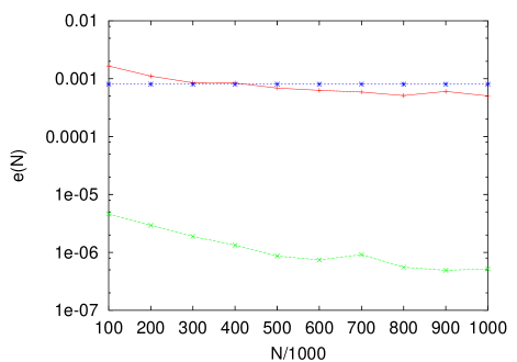
which is the error averaged over $M+1$ different pairs of (input,output) angles for a fixed number $N$ of input messages. Fig. 8 shows the error $e(N)$ as a function of the number of events $N$. In this case, $\cos^{2}(\psi_{m}-\phi)$ and $\sin^{2}(\psi_{m}-\phi)$ are rational numbers and the results of Fig. 8 confirm that the DLM performs very well, much better than the probabilistic processor. Fig. 8 also shows that replacing the update rule Eq. (26) by Eq. (51) has a large impact on the performance of a deterministic learning machine.

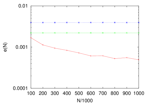
If we replace $\psi_{m}-\phi=\arcsin\sqrt{m/M}$ by $\psi_{m}-\phi=m\pi/2M$ in step 4 of the procedure described earlier, then $\sin^{2}(\psi_{m}-\phi)$ is not necessarily a rational number and this affects the performance of the DLM, as shown in Fig. 9. A closer look at the DLM data for different $m$ (results not shown) reveals that the large increase of the error is due to the relatively poor accuracy for $m\approx 0$ and $m\approx M$. This is hardly a surprise: From Sections III.2.2 and III.2.4 we know that the choice of $\alpha$ is more important for $\theta\approx n\pi/2$ than it is for $\theta\approx n\pi/2+\pi/4$. Therefore, if optimal performance for all $\theta$ is crucial, it is necessary to adjust $\alpha$ dynamically by another learning process. We leave this topic for future research.

Figure 10: (color online) Snapshot of the event-by-event simulator of two concatenated Mach-Zehnder interferometers MZIdemo . The main panel shows the layout of the interferometer. Particles emerge from a source (not shown) located at the bottom of the left-most vertical line. After leaving the first beam splitter in either the vertical or horizontal direction, the particles experience time delays that are specified by the controls on the lines. In this example, the time delays correspond to the phase shifts $\phi_{0}=152^{\circ}$, $\phi_{1}=302^{\circ}$, $\phi_{2}=0^{\circ}$, and $\phi_{3}=342^{\circ}$ in the quantum mechanical description. The thin, $45^{\circ}$-tilted lines act as perfect mirrors. When a particle leaves the system at the top right, it adds to the count of either detector $N_{4}$ or $N_{5}$. Additional detectors ($N_{0}$, $N_{1}$, $N_{2}$, and $N_{3}$) count the number of particles on the corresponding lines. The other cells give the ratio of the detector counts to the total number of particles (messages) processed and also the corresponding probability of the quantum mechanical description. At any time, the user can choose between a strictly deterministic and a probabilistic event-by-event simulation by pressing the buttons at the top of the control panel.

IV Relevance of the learning process

The fundamental difference between the simple probabilistic processor of Section II and the DLM of Section III is that the latter has a learning capability. Elsewhere, we have shown that learning is an essential ingredient of networks of probabilistic or deterministic processors that are able to simulate, event-by-event, quantum interference phenomena and universal quantum computation KRAED05 ; HRAED05a ; MICH05 ; HRAED05b . The fundamental reason for this is that some form of communication between individual events is required in order to simulate (classical or quantum) interference phenomena. Although the Bernoulli-type probabilistic processor of Section II satisfies our criteria 1 and 2 of Section I for an efficient processor, it generates uncorrelated events and any form of communication between events is absent. Therefore the probabilistic processor of Section II cannot simulate interference phenomena but the DLM of Section III can because it has the additional feature of being able to learn from previous events.

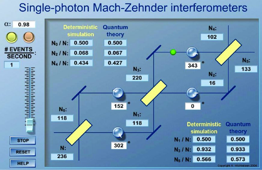
As a non-trivial illustration of the importance of the learning process, we consider the interferometer depicted in Fig. 10 MZIdemo . This interferometer consists of two chained Mach-Zehnder interferometers BORN64 . Photons leave the source (not shown) located at the bottom of the left-most vertical line. The beam splitters, represented by the large rectangles, transmit or reflect photons with probability 1/2. After leaving the first beam splitter in the vertical or horizontal direction, the photons experience a time delay that is determined by the length of the optical path from one beam splitter to the next. The length of each path is variable, as indicated schematically by the controls on the horizontal lines. In a wave mechanical description, the time delays correspond to changes in the phase of the wave. The thin, $45^{\circ}$-tilted lines act as perfect mirrors.

In quantum theory, the presence of photons in the input modes 0 or 1 of the interferometer is represented by the probability amplitudes ($a_{0},a_{1})$ BAYM74 . According to quantum theory, the amplitudes ($b_{0},b_{1})$ of the photons in the output modes 0 and 1 of a beam splitter are given by BAYM74

$$\left(\begin{array}[]{c}b_{0}\\ b_{1}\end{array}\right)=\frac{1}{\sqrt{2}}\left(\begin{array}[]{cc}1&i\\ i&1\end{array}\right)\left(\begin{array}[]{c}a_{0}\\ a_{1}\end{array}\right).$$ (59)

The amplitudes to observe a photon in the output modes 0 and 1 of one Mach-Zehnder interferometer of Fig. 10 are given by

$$\left(\begin{array}[]{c}b_{2}\\ b_{3}\end{array}\right)=\left(\begin{array}[]{cc}1&i\\ i&1\end{array}\right)\left(\begin{array}[]{cc}e^{i\phi_{0}}&0\\ 0&e^{i\phi_{1}}\end{array}\right)\left(\begin{array}[]{c}b_{0}\\ b_{1}\end{array}\right).$$ (68)

The amplitudes to observe a photon in the output modes 0 and 1 of two chained Mach-Zehnder interferometers are given by

$$\left(\begin{array}[]{c}b_{4}\\ b_{5}\end{array}\right)=\left(\begin{array}[]{cc}1&i\\ i&1\end{array}\right)\left(\begin{array}[]{cc}e^{i\phi_{2}}&0\\ 0&e^{i\phi_{3}}\end{array}\right)\left(\begin{array}[]{c}b_{2}\\ b_{3}\end{array}\right).$$ (77)

In Eqs. (68) and (77), the entries $e^{i\phi_{j}}$ for $j=0,1,2,3$ implement the phase shifts that result from the time delays on the corresponding path (including the phase shifts due to the presence of the perfect mirrors). The probability to detect a photon in either output mode 0 or 1 of the two chained Mach-Zehnder interferometers are given by $|b_{4}|^{2}$ or $|b_{5}|^{2}$, respectively.

Using DLM networks, it is possible to reproduce the wave-like behavior by an event-by-event, particle-like, simulation without using wave mechanics KRAED05 ; HRAED05a ; MICH05 ; HRAED05b . Elsewhere KRAED05 ; HRAED05a ; MICH05 ; HRAED05b we have shown that DLM networks can simulate, event by event, single-photon beam splitter and (modified) Mach-Zehnder interferometer experiments GRAN86 ; BRAI03 .

Fig. 10 shows the schematic diagram of the DLM network that performs the event-by-event simulation of the two chained Mach-Zehnder interferometers MZIdemo . Particles emerge one-by-one from a source (not shown) located at the bottom of the left-most vertical line. At any time, there is at most one particle (represented by the small sphere) in the system. The number of particles that have left the source is given by $N$.

Each particle carries its own clock. There is a one-to-one correspondence between the direction of the hand of the clock and the message ${\bf y}_{n+1}=(y_{1,n+1},y_{2,n+1})$. The clock is read and manipulated by the beam splitters, represented by the large rectangles. Each beam splitter contains two DLMs KRAED05 . The internal structure of the DLM network that performs the task of a beam splitter is described in detail elsewhere KRAED05 ; HRAED05a ; MICH05 ; HRAED05b , so there is no need to repeat it here. Of course, these networks are the same for the three beam splitters.

After leaving the first beam splitter in either the vertical or horizontal direction (but never in both), the particle experiences a time delay that is determined by the controls on the lines. This time delay is implemented as a rotation of the hand of the particle’s clock. When a particle leaves the system at the top right, it adds to the count of either detector $N_{4}$ or $N_{5}$. Additional detectors ($N_{0}$, $N_{1}$, $N_{2}$, and $N_{3}$) count the number of particles on the corresponding lines. The label of $\phi_{j}$ in the quantum mechanical description is the same as the label of the corresponding counter $N_{j}$. The other cells give the ratio of the detector counts to the total number of particles (messages) processed and also the corresponding probability of the quantum mechanical description. At any time, the user can choose between a strictly deterministic and a probabilistic event-by-event simulation by pressing the buttons at the top of the control panel. We emphasize that this DLM-based simulation is dynamic and adaptive in all respects: During the simulation, the user can change any of the controls and after a short transient period, the DLM-network generates output events according to the quantum mechanical probabilities.

The snapshot in Fig. 10 is taken after $N=236$ particles have been generated by the source (with one particle still under way). The numbers in the various corresponding fields clearly show that even after a modest number of events, this event-by-event simulation reproduces the quantum mechanical probabilities. Of course, this single snapshot is not a proof that the event-by-event simulation also works for other choices of the delays.

An event-by-event simulation correctly reproduces the quantum mechanical probabilities if and only if $N_{j}/N\approx|b_{j}|^{2}$ for $j=0,1,2,3$, for any choice of the delays (phases) $\phi_{j}$. Very extensive tests, reported elsewhere KRAED05 ; HRAED05a ; MICH05 ; HRAED05b demonstrate that DLM-networks accurately reproduce the probabilities of the quantum theory.

In the event-by-event simulation, interference is a direct result of the learning process that takes place in each DLM. In the case at hand, the three (identical) beam splitters contain the learning machines. We emphasize that there is no direct communication between the different beam splitters. All the information is carried by the particle while it is routed through the network. This is essential for the simulation to satisfy the physical criterion of causality.

V Summary

In this paper we ask ourselves the question what the optimal design of a processor, which can process and count incoming individual objects carrying information represented by an angle $\psi$ but which cannot measure $\psi$ directly, would be if it has to give the most accurate estimate of the angle $\psi$. In other words, how can we simulate the operation of a photon polarizer?

First, we construct a processor operating according to the rules of probability theory. This so-called probabilistic processor uses random numbers to transform the incoming angle $\psi$, that is the information carried by the incoming single objects, into a sequence of discrete output events labeled by $\pm 1$. The numbers of $+1$ and $-1$ events only depend on the difference $\theta=\psi-\phi$ between the unknown angle $\psi$ and the orientation $\phi$ of the processor. We design the probabilistic processor such that the result of the transformation process is probabilistic (Bernoulli trials), rotational invariant and satisfies the criteria 1 and 2 of Section I. For fixed $\phi$ and $N$ incoming objects, the observer, using the probabilistic processor to measure $\psi$ as accurate as possible, will get most out of the data if the processor sends $N\cos^{2}\theta$ ($N\sin^{2}\theta$) events to the apparatus that detects the $+1$ ($-1$) events. The number of angles $\theta$ that the observer can distinguish is proportional to $\sqrt{N}$. The probabilistic processor is thus a model for an ideal polarizer. It produces data that agrees with Malus ’ law. However, it is important to note that to obtain this result we do not use any law of physics in the design of the processor. We do not use the probability distributions derived in quantum theory to generate the $\pm 1$ events but we design the probabilistic processor in such a way that these probability distributions come out as a result of efficient processing of incoming data by the processor. Hence, we can ask the following important question. Can also other quantum phenomena appear as a result of efficient data processing?

In order to answer this question we follow another route. Although the Bernoulli type probabilistic processor can simulate the classical and quantum properties of a photon polarizer, it cannot simulate interference phenomena. To overcome this problem we could design a probabilistic processor that does not generate Bernoulli events but correlated output events. However, we choose to design processors that use a deterministic algorithm with a primitive learning capability to transform the incoming events into a sequence of discrete output events. This type of processors we call deterministic processors or deterministic learning machines.

Therefore, as a second step, we construct a deterministic processor that models a photon polarizer, that is a deterministic processor that generates output events according to Malus’ law. Just as the probabilistic processor, the deterministic processor has one input channel and two output channels labeled by $+1$ and $-1$, respectively. Apart from this the deterministic processor also has an internal vector with two real entries. The input messages to the deterministic processor are unit vectors ${\bf y}_{n+1}=(\cos\theta_{n+1},\sin\theta_{n+1})$ for $n=0,\ldots,N$ and where $\theta_{n}=\psi_{n}-\phi$. The deterministic processor learns from the input events by updating its internal vector and uses this internal vector in a completely deterministic decision process to send out a $+1$ or a $-1$ event. Hence, the order in which the $+1$ and $-1$ events are sent is deterministic. Apart from being deterministic, the result of the transformation process is rotational invariant and satisfies criteria 1 and 2 of Section I, which are exactly the same requirements as the ones used to construct the probabilistic processor. Further analysis of the output events shows that the number of $+1$ and $-1$ output events agrees with Malus’ law. Hence, the photon polarizer can also be modelled by a deterministic processor. As in the case of the probabilistic processor, also in this case we did not use any laws of physics to design the processor. The number of angles $\theta$ that the observer, using the deterministic processor to measure $\psi$, can distinguish is equal to $N+1$. Hence, in this respect the deterministic processor performs much better than the probabilistic one. However, the more important and fundamental difference between the probabilistic and the deterministic processor is that the latter has a learning capability. Learning is an essential ingredient to simulate interference phenomena since it correlates the output events. As an example we show the event-by-event simulation of photons routed through two chained Mach-Zehnder interferometers by using a network of deterministic processors. We show that the quantum mechanical probabilities are also reproduced for this interference experiment.

In conclusion, processors that efficiently process incoming data in the form of single events can simulate some quantum phenomema, such as the recovery of Malus’ law for a photon polarizer. However, in order to simulate quantum interference the processor should in addition have the capability of learning. Most importantly, the present work demonstrates that viewing quantum systems as efficient data processors provides a framework to construct adaptive, dynamical systems that can simulate quantum interference on an event-by-event basis, without using concepts of quantum theory.

Appendix A On the use of the Cramér-Rao inequality

In Frieden’s approach the Cramér-Rao inequality plays a central role to motivate the use of the Fisher information as a measure of the expected error in measurements FRIE99 . From probability theory it is well known that the Cramér-Rao inequality sets a lower bound to the variance of an estimator TREE68 ; FRIE99 ; JAYN03 . Here we prove that, within the limitations set by our design criteria, the estimation procedure is efficient in the sense that it satisfies the Cramér-Rao inequality with equality TREE68 ; FRIE99 and that this inequality reduces to a trivial identity that contains no information JAYN03 . For convenience of the reader, we repeat the derivation of the Cramér-Rao inequality for the case of interest.

Writing Eq.(2) as

$$\sum_{x=\pm 1}(x-f(\theta))p(x|\theta)=0,$$ (78)

and taking the derivative with respect to $\theta$ we obtain

$$\sum_{x=\pm 1}(x-f(\theta))\frac{\partial p(x|\theta)}{\partial\theta}=\frac{\partial f(\theta)}{\partial\theta}.$$ (79)

Rewriting Eq.(79) as

$$\sum_{x=\pm 1}\left[(x-f(\theta))\sqrt{p(x|\theta)}\right]\left[\frac{1}{\sqrt{p(x|\theta)}}\frac{\partial p(x|\theta)}{\partial\theta}\right]=\frac{\partial f(\theta)}{\partial\theta},$$ (80)

and using the Schwartz inequality gives the Cramér-Rao inequality

$$\left\{\sum_{x=\pm 1}(x-f(\theta))^{2}p(x|\theta)\right\}\left\{\sum_{x=\pm 1}\frac{1}{p(x|\theta)}\left[\frac{\partial p(x|\theta)}{\partial\theta}\right]^{2}\right\}=\hbox{Var}(x)I_{F}\geq\left(\frac{\partial f(\theta)}{\partial\theta}\right)^{2}.$$ (81)

where

$$I_{F}=\sum_{x=\pm 1}\frac{1}{p(x|\theta)}\left[\frac{\partial p(x|\theta)}{\partial\theta}\right]^{2},$$ (82)

is the Fisher information TREE68 ; FRIE99 ; BLAH91 . With the use of Eq.(1) we can write $I_{F}$ as

$$I_{F}=\frac{1}{p(1|\theta)(1-p(1|\theta))}\left[\frac{\partial p(1|\theta)}{\partial\theta}\right]^{2},$$ (83)

which is identical to Eq. (11). Any estimation procedure that satisfies the bound in Eq. (81) with equality is called efficient TREE68 ; FRIE99 . Using Eq. (2) and $\hbox{Var}(x)=\langle x^{2}\rangle-\langle x\rangle^{2}=4p(1|\theta)(1-p(1|\theta))$ we find

$$\hbox{Var}(x)I_{F} = 4\left[\frac{\partial p(1|\theta)}{\partial\theta}\right]^{2}=\left[\frac{\partial f(\theta)}{\partial\theta}\right]^{2}.$$ (84)

Hence, the inequality Eq. (81) reduces to a trivial identity from which we cannot deduce anything useful JAYN03 .

References

- (1) G. Baym, Lectures on Quantum Mechanics, W.A. Benjamin, Reading MA (1974).
- (2) R.P. Feynman, R.B. Leighton, M. Sands, The Feynman lectures on Physics, Vol. 3, Addison-Wesley, Reading MA (1996).
- (3) M. Born and E. Wolf, Principles of Optics, Pergamon, Oxford (1964).
- (4) D. Home, Conceptual Foundations of Quantum Physics, Plenum Press, New York (1997).
- (5) These constraints simply express the known, basic properties of the photon polarization BORN64 ; BAYM74 .
- (6) G.R. Grimmet and D.R. Stirzaker, Probability and Random Processes, Clarendon Press, Oxford UK (1995).
- (7) M. Tribus, Rational Descriptions, Decisions, and Designs, Expira Press, Stockholm Sweden (1999).
- (8) E.T. Jaynes, Probability Theory: The Logic of Science, Cambridge University Press, Cambridge UK (2003).
- (9) H.L. Van Trees, Detection, Estimation, and Modulation Theory (Part I), Wiley, New York (1968).
- (10) B.R. Frieden, Physics from Fisher information: a unification, Cambridge University Press, Cambridge UK (1999).
- (11) R.E. Blahut, Principles and Practice of Information Theory, Addison-Wesley, Reading Massachussets (1991).
- (12) W.K. Wootters, Phys. Rev. D 23, 357 (1981).
- (13) J. Summhammer, in Foundations of Probability and Physics, A. Khrennikov, Ed., World Scientific, Singapore (2001).
- (14) K. De Raedt, H. De Raedt, and K. Michielsen, Comp. Phys. Comm. (in press).
- (15) H. De Raedt, K. De Raedt, and K. Michielsen, J. Phys. Soc. Jpn. Suppl. 74, 16 - 25 (2005).
- (16) K. Michielsen, K. De Raedt, and H. De Raedt, J. Comp. Theor. Nanoscience 2, 1 (2005).
- (17) H. De Raedt, K. De Raedt, and K. Michielsen, Europhys. Lett. 69, 861 (2005).
- (18) S. Haykin, Neural Networks, Prentice Hall, New Jersey (1999).
- (19) M.H. Jensen, P. Bak, and T. Bohr, Phys. Rev. Lett. 50, 1637 (1983).
- (20) J. Hubbard, Phys. Rev. B 17, 494 (1978).
- (21) Fortran and Java programs and interactive programs that perform event-based simulations of a beam splitter, one Mach-Zehnder interferometer, and two chained Mach-Zehnder interferometers can be found at http://www.compphys.net/dlm
- (22) P. Grangier, R. Roger, and A. Aspect, Europhys. Lett. 1, 173 (1986).
- (23) Ch. Braig, P. Zarda, C. Kurtsiefer, and H. Weinfurter, Appl. Phys. B 76, 113 (2003).