To Janine and Isabel

Abstract

By taking advantage of the laws of physics it is possible to revolutionize the way we communicate (transmit), process or even store information. It is now known that quantum computers, or computers built from quantum mechanical elements, provide new resources to solve certain problems and perform certain tasks more efficiently than today’s conventional computers. However, on the road to a complete understanding of the power of quantum computers there are intermediate steps that need to be addressed. The primary focus of this thesis is the understanding of the possibilities and limitations of the quantum-physical world in the areas of quantum computation and quantum information processing.

First I investigate the simulation of quantum systems on a quantum computer (i.e., a quantum simulation) constructed of two-level quantum elements or qubits. For this purpose, I present algebraic mappings that allow one to efficiently obtain physical properties and compute correlation functions of fermionic, anyonic, and bosonic systems with such a computer. By studying the amount of resources required for a quantum simulation, I show that the complexity of preparing a quantum state which contains the desired information is crucial at the time of evaluating the advantages of having a quantum computer over a conventional one. As a small-scale demonstration of the validity of these results, I show the simulation of a fermionic system using a liquid-state nuclear magnetic resonance (NMR) device.

Remarkably, the conclusions obtained in the area of quantum simulations can be extended to general quantum computations by means of the notion of generalized entanglement. This is a generalization based on the idea that quantum entanglement (i.e., the existence of non-classical correlations) is a concept that depends on the accesible information, that is, relative to the observer. Then I present a wide class of quantum computations that can be efficiently simulated on a conventional computer and where quantum computers cannot be claimed to be more powerful. The idea is that a quantum algorithm, performed by applying a restricted set of gates which do not create generalized entangled states relative to small (polynomially-large) sets of observables, can be imitated using a similar amount of resources with a conventional computer. However, a similar statement cannot be obtained when generalized entangled states (relative to these sets) are involved, because this purely quantum phenomena cannot be easily reproduced by classical-information methods.

Finally, I show how these concepts developed from an information-theory point of view can be used to study other important problems in many-body physics. To begin with, I exploit the notion of Lie-algebraic purity to identify and characterize the quantum phase transitions present in the Lipkin-Meshkov-Glick model and the spin-1/2 anisotropic XY model in a transverse magnetic field. The results obtained show how generalized entanglement leads to useful tools for distinguishing between ordered and disordered phases in quantum systems. Moreover, I discuss how the concept of general mean field hamiltonians naturally emerges from these considerations and show that these can be exactly diagonalized by using a conventional computer.

In brief, in this thesis I apply several topics developed in the context of quantum information theory to study the complexity of obtaining relevant physical properties of quantum systems with a quantum computer, and to study different physical processes in quantum many-body systems.

Chapter 1 Introduction

…there is plenty of room to make computers smaller…nothing that I can see in the physical laws…

R. P . Feynman, Caltech (1959).

During the last few decades, the theory of Quantum Information Processing (QIP) has acquired great importance because it has been shown that information based on quantum mechanics provides new resources that go beyond the traditional ‘classical information’. It is now known that certain quantum mechanical systems, named quantum computers (QCs), can be used to easily solve certain problems which are difficult to solve using today’s conventional or classical computers CCs. Having a QC would allow one to communicate in secret [BB84] (quantum cryptography), perform a variety of search algorithms [Gro97], factor large numbers [Sho94], or simulate efficiently some physical systems [OGK01, SOG02]. Additionally, it would allow us to break security codes used, for example, to secure internet communications, optimize a large variety of scheduling problems, etc., which make of quantum information an exciting and relevant subject. Consequently, the science of quantum information is mainly focused on better understanding the foundations of quantum mechanics (which are different of classical mechanics) and the physical realization of quantum controllable physical devices. While the first allows clever and not so obvious ways of taking advantage of the quantum world, the latter will let us achieve our most important goal: the building of a QC.

When one looks for the word information in the dictionary one finds many definitions: i) a message received and understood, ii) knowledge acquired through study or experience, iii) propagated signal through a given channel, iv) broadcasted news, and more. Information is then the basis of all human knowledge and we usually base our behavior on it. It always requires a physical representation to be able to use it, propagate it, or store it, such as a telephone, a computer disk, etc. Depending on the physical representation, information can be classical or quantum.

We define as classical information the one that is manipulated and stored by today’s CCs. In classical information theory the basic unit is the bit. A bit’s state can be in one of two states represented by the numbers 0 and 1, which constitute the logical basis. A possible physical representation of a bit is given by a system in which the state is determined by the distribution of, for example, electrical charge. The idea is then to process information through the manipulation of the state of a set of bits (i.e., bit sequence) by performing elementary gates. These gates are different processes that depend on the particular physical realization of the CC.

Examples of one-bit gates are the not and reset gates, and of two-bit gates is the nand gate. Their action over logical initial states are shown in Fig. 1.1. They suffice for implementing arbitrary state transformations. That is, any classical algorithm can be implemented through a circuit that consists of applying these elementary gates to a bit sequence. In fact, this method is used by today’s computers, where the program sets up a particular order for performing the elementary gates and the chips implement them physically. Finally, one reads the final state where the required information is supposed to be encoded (e.g., the solution to a problem).

Figure 1.1: Logical action of the single bit gates not and reset, and the two-bit gate nand. Here is and fs denote the initial and final bit states, respectively.

The idea of quantum information processing is similar to that of classical information but under the laws of the quantum world. One defines quantum information as the one which is stored and manipulated by physical devices obeying the laws of quantum physics; that is, satisfying the Schrödinger evolution equation

$$i\hbar\frac{d}{dt}|{\psi}\rangle=H|{\psi}\rangle,$$ (1.1)

where $H$ is the Hamiltonian describing the interactions that one manipulates to perform the desired evolution, and $|{\psi}\rangle$ is some pure state (i.e., wave function) of the system. Such devices constitute quantum computers.

In the conventional model of quantum information theory (QIT) the basic unit is the quantum bit or qubit. A qubit’s pure state can be in any superposition of the logical states and is expressed as $a|{0}\rangle+b|{1}\rangle$, where the complex numbers $a$ and $b$ are the probability amplitudes of being in the states $|{0}\rangle$ and $|{1}\rangle$, respectively. They are normalized to the unity: $|a|^{2}+|b|^{2}=1$. A possible physical representation of a qubit is given by any two-level quantum system (Fig. 1.2) such as a spin-1/2, where the state represented by $|{0}\rangle$ ($|{1}\rangle$) corresponds to the state with the spin pointing up (down), or a single atom. Bohm’s rule [Boh51] tells one that such state corresponds to having probabilities $|a|^{2}$ and $|b|^{2}$ of being in the state with the spin pointing up and down, respectively.

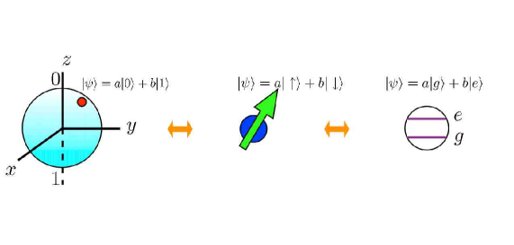
Figure 1.2: Different physical representations of the single qubit state $|{\psi}\rangle=a|{0}\rangle+b|{1}\rangle$. The red dot on the surface of the sphere (left) represents such a linear combination of states. Here $|{g}\rangle$ and $|{e}\rangle$ denote the ground and an excited state of a certain atom.

Due to the superposition principle of quantum physics, a pure state of a set of $N$ qubits (register) is expressed as $a_{0}|{0\cdots 00}\rangle+a_{1}|{0\cdots 01}\rangle+\cdots+a_{2^{N}-1}|{1\cdots 11}\rangle$. Again, the complex coefficients $a_{i}$ are the corresponding probability amplitudes, and $\sum_{i}|a_{i}|^{2}=1$. The idea is then to perform computation by executing a quantum algorithm that consists of performing a set of elementary gates in a given order (i.e., a quantum circuit). The action of these quantum gates is rigorously discussed in Chap. 2 and requires some previous knowledge in linear algebra. As in classical information, these gates involve single qubit and two-qubit operations. In order to preserve the features of quantum physics, these operations must be reversible (i.e., unitary operations), and are usually performed by making the register interact with external oscillating electromagnetic fields.

The great advantages of having a QC are two-fold: First, working at the quantum level allows one to make these computers extremely small and, if scalable [Div95], it would allow one to process a large number of qubits at the same time. Second, a computer ruled by the laws of quantum physics should contain certain features that go beyond those of classical information, since the latter can be considered a limit of the first one. For example, one immediately observes that the superposition principle gives one more freedom when manipulating quantum information, in the sense that many different logical states can be carried simultaneously (parallelism).

To analyze the computational complexity to solve a certain problem one needs to determine the total amount of physical resources required, such as bits or qubits, the number of operations performed or number of elementary gates, the number of times that the algorithm is executed, etc. While nobody knows yet the power of quantum computation, certain algorithms [Sho94, Gro97] suggest that QCs are more powerful than their classical analogues. All these algorithms share the feature that they not only make use of the superposition principle (which is not sufficient to claim that a QC is more efficient), but also of the non-classical correlations between different quantum elements in the QC. (Interference phenomena also plays an important role in the efficiency of quantum algorithms.) Such correlations are inherent to quantum systems [Sch35, EPR35] and do not exist in classical systems. They are usually referred as quantum entanglement (QE), an emerging field of QIT.

In order to access the quantum information, one needs to perform a measurement. This is defined as the extraction of some classical information from the quantum register. Due to the features of quantum physics, after a measurement process the state of the register is collapsed into the logical state corresponding to the outcome, with statistics given by Bohm’s rule (Fig. 1.3). This process could destroy the efficiency of the computation. For example, if after the execution of the quantum algorithm the state of two qubits is $a_{0}|{00}\rangle+a_{1}|{01}\rangle+a_{2}|{10}\rangle+a_{3}|{11}\rangle$, a measurement process in the logical basis has the effect of collapsing the state to $|{00}\rangle$ with probability $|a_{0}|^{2}$, to $|{01}\rangle$ with probability $|a_{1}|^{2}$, to $|{10}\rangle$ with probability $|a_{2}|^{2}$, and to $|{11}\rangle$ with probability $|a_{3}|^{2}$. Therefore, a single measurement does not give the whole information about the state of the register and usually one needs to run the quantum algorithm repeatedly many times to obtain more accurate statistics to recover the state of the register. This is a main difference with the case of classical information, where such measurement or convertion is not necessary.

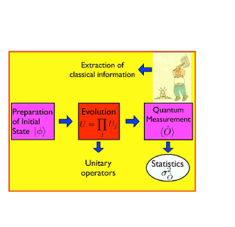
Figure 1.3: Circuit representation of a quantum algorithm. A pure state $|{\psi}\rangle$ is evolved by applying elementary gates. The evolution obeys Schrödinger’s equation (Eq. 1.1). After the evolution, a measurement collapses the evolved state with statistics given by Bohm’s rule.

The simplest case of an entangled state is the pure two-qubit state (Fig. 1.4)

$$|{\psi}\rangle=\frac{1}{\sqrt{2}}[|{10}\rangle+|{01}\rangle],$$ (1.2)

or similar states obtained by flipping or by changing the phase of a single qubit. Equation 1.2 states that if one qubit is measured and projected in the logical basis, the other qubit is automatically projected in the same basis. Moreover, if the outcome of a measurement performed in one qubit is 0 (1), the outcome of a post-measurement performed on the other qubit will be 1 (0). Remarkably, similar results are obtained for such state if the measurements are performed in a basis other than the logical one. These correlations between outcomes cannot be explained by a classical theory.

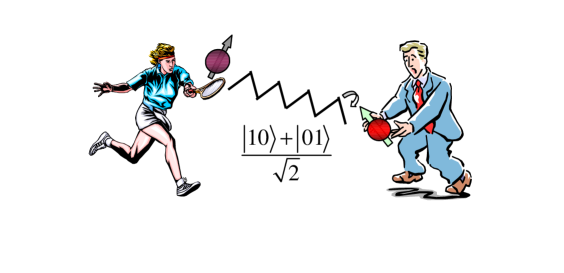
Figure 1.4: Maximally entangled two-qubit state. The quantum correlations cannot be represented by any classical state.

During the last few years, several authors [EHK04, GK, SOK03, Val02, Vid03] have started to study the relation between different definitions and measures of QE and quantum complexity. Naturally, they mostly agreed that whenever the QE of the evolved state in a quantum computation is small enough, such algorithms can be simulated with the same efficiency on a CC. However, the lack of a unique computable measure of entanglement that could be applied to any quantum state and quantum system is the main reason why the power of QCs is still not fully understood.

One of the purposes of my thesis is to show the computational complexity (i.e.., the number of resources and operations needed) to solve certain problems with QCs and to compare it with the corresponding classical complexity. In particular, I will first focus on the study of the simulation of physical systems by quantum networks or quantum simulations (QSs) [OGK01, SOG02, SOK03]. As noticed by R. P. Feynman [Fey82] and Y. Manin, the obvious difficulty with deterministically solving a quantum many-body problem (e.g., computing some correlation functions) on a CC is the exponentially large basis set needed for its simulation. Known exact diagonalization approaches like the Lanczos method suffer from this exponential catastrophe. For this reason, it is expected that using a computer constructed of distinct quantum mechanical elements (i.e., a QC) that ‘imitates’ the physical system to be simulated (i.e., simulates the interactions) would overcome this difficulty.

The results obtained by studying the complexity of QSs can be extended to understand the complexity of solving other problems. For example, different quantum search algorithms [Gro97] admit a Hamiltonian representation and can be equivalently considered as a particular QS. But most importantly, I will show how these simulations lead to the definition of a general measure of quantum (pure state) entanglement, so called generalized entanglement (GE), which can be applied to any quantum state regardless of its nature. Remarkably, this measure is crucial when analyzing the efficiency-related advantages of having a QC.

This report arises from the studies and novel results obtained together with my colleagues at Los Alamos National Laboratory (USA) and Instituto Balseiro (Argentina) during my PhD studies. For a better understanding, the main results are presented in chronological order. In Chap. 2, I analyze the problem of simulating different finite physical systems on a QC using deterministic quantum algorithms. The corresponding computational complexity is also studied. As a proof of principles, I present the experimental simulation of a particular fermionic many-body system on a liquid-state nuclear-magnetic-resonance (NMR) QC.

In Chap. 3, I introduce the concept of quantum generalized entanglement, a notion that goes beyond the traditional quantum entanglement concept and makes no reference to a particular subsystem decomposition. I show that important results are obtained whenever a Lie algebraic setting exists behind the problem under consideration. In particular, I apply this novel approach to the study of quantum correlations in different quantum systems, regardless of their nature or particle statistics, including different spin and fermionic systems.

In Chap. 4 I compare the effort of simulating certain quantum systems with a QC or a CC. In particular, I show that the concept of generalized entanglement is crucial to the efficiency of a quantum algorithm and can be used as a resource in quantum computation. Moreover, generalized entanglement allows one to make a connection between QIT and many-body physics by studying different problems in quantum mechanics, such as the characterization of quantum phase transitions in matter or the study of integrable quantum systems. These results are presented in Chap. 5.

Finally, in Chap. 6, I present the conclusions, open questions, and future directions related to this subject.

Chapter 2 Simulations of Physics with Quantum Computers

Since Richard P. Feynman conjectured that an arbitrary discrete quantum system may be simulated by another one [Fey82], the simulation of quantum phenomena became a fundamental problem that a quantum computer (QC), i.e., a system of universally controlled distinct quantum elements, may potentially solve in a more efficient way than a classical computer (CC). The main problem with the simulation of a quantum system on a CC is that the dimension of the associated Hilbert space grows exponentially with the volume of the system to be simulated. For example, the classical simulation of a system composed of $N$ qubits requires, in general, an amount of computational operations (additions and products of complex numbers) that is proportional to $D=2^{N}$, where $D$ is the dimension of the Hilbert space given by the number of different logical states $|{i_{1}i_{2}\cdots i_{N}}\rangle$, with $i_{j}=\{0,1\}$. Nevertheless, a QC allows one to imitate the evolution of the corresponding quantum system by cleverly controlling and manipulating its elements. This process is called a quantum simulation (QS). It is expected then that the number of resources required for the QS increases linearly (or at most, polynomially) with the volume of the system to be simulated [AL97]. If this is the case, we say that the QS can be performed efficiently.

To be able to perform a QS, it is necessary to make a connection between the operator algebra associated to the system and the operator algebra which defines the model of quantum computation [OGK01]. The existence of one-to-one mappings between different algebras of operators and one-to-one mappings between different Hilbert spaces [BO01, SOK03], is a necessary requirement to simulate a physical system using a QC built on the basis of another system (Fig. 2.1). For example, one can simulate a fermionic system on a liquid-state nuclear magnetic resonance (NMR) QC by making use of the Jordan-Wigner transformation [JW28] that maps fermionic operators onto the Pauli (spin-1/2) operators. Although these mappings can usually be performed efficiently, this is not sufficient to establish that any system can be simulated efficiently on a QC. It is then necessary to prove that all steps involved in the QS, including the initialization, evolution, and measurement, can be performed efficiently [SOG02].

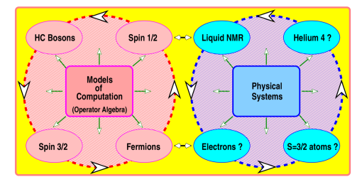
Figure 2.1: Relationship between different models of computation (with their associated operator algebras) and different physical systems. Question marks refer to the present lack of a quantum computer device using the corresponding elementary physical components indicated in the box. Diamond-shaped arrows represent the natural connection between physical system and operator language, while arrows on the circle indicate the existence of isomorphisms of $*$-algebras, therefore, the corresponding simulation of one physical system by another.

This chapter will explore the theoretical and experimental issues associated with the simulations of physical phenomena on QCs. In Sec. 2.1, I start by describing different models of quantum computation. In particular, I rigorously introduce the conventional model by means of the Pauli operators, where a natural set of elementary gates (i.e., set of universal operations) is obtained. This model, roughly described in Chap. 1, is the one generally needed for the practical implementation of a QS. In Sec. 2.2, I present a class of quantum algorithms (QAs) in the language of the conventional model, for the computation of relevant physical properties of quantum systems, such as correlation functions, energy spectra, etc. In Sec. 2.3, I explain how the QS of quantum physical systems obeying fermionic, anyonic, and bosonic particle statistics, can be performed on a QC described by the conventional model, presenting some mappings between the different operator algebras. As an application, in Sec. 2.4 I show the QS (imitated by a classical computer) of a particular fermionic system: The two-dimensional fermionic Hubbard model. It is expected that such simulation gives an insight into the limitations of quantum computation, showing that certain issues remain to be solved to assure that a QC is more powerful than a CC (Sec. 2.5). In Sec. 2.7, I describe the experimental implementation on an NMR QC of the QS of another fermionic system: The Fano-Anderson model. For this purpose, an elementary introduction to the physical processes on an NMR setting is described in Sec. 2.6. Finally, I summarize in Sec. 2.8.

2.1 Models of Quantum Computation

When performing a quantum computation, the quantum elements which constitute the QC can be universally controlled and manipulated by modulating and changing their interactions. This quantum control model assumes then the existence of a control Hamiltonian $H_{P}$, which describes these interactions. The control possibilities are used to implement specific quantum gates, allowing one, for example, to represent the time evolution of the physical system to be simulated [OGK01].

In order to define a model of quantum computation it is necessary to give a physical setting together with its initial state, an algebra of operators associated to the system, a set of controllable Hamiltonians necessary to define a set of elementary gates, and a set of measurable operators (i.e., observables). In this way, many different models of quantum computation can be described, but for historic reasons and practical purposes I will focus mostly on the conventional model [NC00].

2.1.1 The Conventional Model of Quantum Computation

As mentioned in Chap. 1, in the conventional model of quantum computation, the fundamental unit of information is the quantum bit or qubit. A qubit’s pure state $|{\sf a}\rangle=a|{0}\rangle+b|{1}\rangle$ (with $a,b\in\mathbb{C}$ and $|a|^{2}+|b|^{2}=1$), is a linear superposition of the logical states $|{0}\rangle$ and $|{1}\rangle$, and can be represented by the state of a two-level quantum system such as a spin-1/2. Assigned to each qubit are the identity operator ${\mathchoice{\rm 1\mskip-4.0mul}{\rm 1\mskip-4.0mul}{\rm 1\mskip-4.5mul}{\rm 1\mskip-5.0mul}}$ (i.e., the no-action operator) and the Pauli operators $\sigma_{x}$, $\sigma_{y}$, and $\sigma_{z}$. In the logical single-qubit basis $\mathcal{B}=\{|{0}\rangle,|{1}\rangle\}$, these are

$${\mathchoice{\rm 1\mskip-4.0mul}{\rm 1\mskip-4.0mul}{\rm 1\mskip-4.5mul}{\rm 1\mskip-5.0mul}}=\pmatrix{1&0\cr 0&1},\ \sigma_{x}=\pmatrix{0&1\cr 1&0},\ \sigma_{y}=\pmatrix{0&-i\cr i&0},\ \sigma_{z}=\pmatrix{1&0\cr 0&-1}.$$ (2.1)

Because of its action over the logical states, the operator $\sigma_{x}$ is usually referred as the flip operator:

$$\sigma_{x}\left\{\matrix{|{0}\rangle\rightarrow|{1}\rangle\ ,\cr|{1}\rangle\rightarrow|{0}\rangle\ .}\right.$$ (2.2)

For practical purposes in this thesis, it is also useful to define the raising (+) and lowering (-) Pauli operators $\sigma_{\pm}=\frac{1}{2}(\sigma_{x}\pm i\sigma_{y})$, and the eigenstates of the flip operator $|{+}\rangle=\frac{1}{\sqrt{2}}[|{0}\rangle+|{1}\rangle]$ and $|{-}\rangle=\frac{1}{\sqrt{2}}[|{0}\rangle-|{1}\rangle]$, satisfying

$$\sigma_{x}|{\pm}\rangle=\pm|{\pm}\rangle.$$ (2.3)

The Pauli operators form the $\mathfrak{su}(2)$ Lie algebra and satisfy the commutation relations ($\mu,\nu,\lambda=\{x,y,z\}$)

$$\left[\sigma_{\mu},\sigma_{\nu}\right]=i2\epsilon_{\mu\nu\lambda}\sigma_{\lambda},$$ (2.4)

where $[A,B]=AB-BA$ and $\epsilon_{\mu\nu\lambda}$ is the total anti-symmetric Levi-Civita symbol. They constitute a complete set of local observables, that is, a basis for the $2\times 2$ dimensional Hermitian matrices with $\sigma_{\mu}=(\sigma_{\mu})^{\dagger}$. The symbol $\dagger$ denotes the corresponding complex conjugate transpose.

Any qubit’s pure state can be represented as a point on the surface of the unit sphere (Bloch-sphere representation) by parametrizing the state as $|{\sf a}\rangle=a|{0}\rangle+b|{1}\rangle=\cos(\theta/2)|{0}\rangle+e^{i\varphi}\sin(\theta/2)|{1}\rangle$ (Fig. 2.2). In order to process a single qubit, a complete set of single-qubit gates has to be given. These operations constitute then, any rotation in the Bloch-sphere representation, which are given by the operators $R_{\mu}(\vartheta)=e^{-i(\vartheta/2)\sigma_{\mu}}=\cos(\vartheta/2){\mathchoice{\rm 1\mskip-4.0mul}{\rm 1\mskip-4.0mul}{\rm 1\mskip-4.5mul}{\rm 1\mskip-5.0mul}}-i\sin(\vartheta/2)\sigma_{\mu}$; that is, a rotation by an angle $\vartheta$ along the $\mu$ axis. These rotations are unitary (reversible) operations, satisfying $R_{\mu}(\vartheta)[R_{\mu}(\vartheta)]^{\dagger}={\mathchoice{\rm 1\mskip-4.0mul}{\rm 1\mskip-4.0mul}{\rm 1\mskip-4.5mul}{\rm 1\mskip-5.0mul}}$ (i.e., no-action), where $R_{\mu}(\vartheta)^{\dagger}\equiv R_{\mu}(-\vartheta)$. This reversibility property allows one to perform these gates with no thermodynamical cost. In Fig. 2.3, I present these elementary single-qubit gates in their circuit representation.

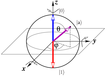
Figure 2.2: Bloch-Sphere representation of a one qubit state parametrized as $|{\sf a}\rangle=\cos(\theta/2)|{0}\rangle+e^{i\varphi}\sin(\theta/2)|{1}\rangle$. The curved arrows denote rotations $R_{\mu}$ along the corresponding axis. The (arrow) color convention is: $|{0}\rangle\rightarrow$ blue; $|{1}\rangle\rightarrow$ red; other linear combinations $\rightarrow$ magenta.

Similarly, a pure state of a $N$-qubit register (quantum register) is represented as the ket $|{\psi}\rangle=\sum_{n=0}^{2^{N}-1}a_{n}|{n}\rangle$, where $|{n}\rangle$ is a product of states of each qubit in the logical (or other) basis, e.g., its binary representation ($|{0}\rangle\equiv|{0_{1}0_{2}\cdots 0_{N}}\rangle,|{1}\rangle\equiv|{0_{1}0_{2}\cdots 0_{N-1}1_{N}}\rangle,|{2}\rangle\equiv|{0_{1}0_{2}\cdots 1_{N-1}0_{N}}\rangle$, etc.), and $\sum_{n=0}^{2^{N}-1}|a_{n}|^{2}=1$ ($a_{n}\in\mathbb{C}$). Assigned to the $j$th qubit of the quantum register are, together with the identity operator ${\mathchoice{\rm 1\mskip-4.0mul}{\rm 1\mskip-4.0mul}{\rm 1\mskip-4.5mul}{\rm 1\mskip-5.0mul}}^{j}$, the local Pauli operators $\sigma_{\mu}^{j}$ (with $\mu=x$, $y$, or $z$); that is

$$\sigma^{j}_{\mu}=\overbrace{{\mathchoice{\rm 1\mskip-4.0mul}{\rm 1\mskip-4.0mul}{\rm 1\mskip-4.5mul}{\rm 1\mskip-5.0mul}}\otimes{\mathchoice{\rm 1\mskip-4.0mul}{\rm 1\mskip-4.0mul}{\rm 1\mskip-4.5mul}{\rm 1\mskip-5.0mul}}\otimes\cdots\otimes\underbrace{\sigma_{\mu}}_{j^{th}\ \mbox{factor}}\otimes\cdots\otimes{\mathchoice{\rm 1\mskip-4.0mul}{\rm 1\mskip-4.0mul}{\rm 1\mskip-4.5mul}{\rm 1\mskip-5.0mul}}}^{n\ \mbox{factors}}\ ,$$

where $\otimes$ represents a Kronecker tensorial product. Their matrix representation in the basis ordered as $\mathcal{B}=\{|{0_{1}\cdots 0_{N-1}0_{N}}\rangle,|{0_{1}\cdots 0_{N-1}1_{N}}\rangle,\cdots,|{1_{1}\cdots 1_{N-1}1_{N}}\rangle\}$ is just the matrix tensor product of the corresponding $2\times 2$ matrices defined by Eq. 2.1. For two different qubits, these operators commute:

$$\left[\sigma_{\mu}^{j},\sigma_{\nu}^{k}\right]=0\ \forall j\neq k.$$ (2.5)

In order to describe a generic operation on the quantum register, it is also necessary to consider products of the Pauli operators $\sigma_{\mu}^{j}$. Remarkably, every unitary (reversible) operation acting on the quantum register can be decomposed in terms of single qubit rotations $R_{\mu}^{j}(\vartheta)=e^{-i\frac{\vartheta}{2}\sigma_{\mu}^{j}}$ and two-qubit gates, such as the Ising gate $R_{z^{j}z^{k}}(\omega)=e^{-i\frac{\omega}{2}\sigma_{z}^{j}\sigma_{z}^{k}}=\cos(\omega/2){\mathchoice{\rm 1\mskip-4.0mul}{\rm 1\mskip-4.0mul}{\rm 1\mskip-4.5mul}{\rm 1\mskip-5.0mul}}-i\sin(\omega/2)\sigma_{z}^{j}\sigma_{z}^{k}$, with $\omega\in\mathbb{R}$ ([BBC95, DiV95]). The operations $R_{z^{j}z^{k}}(\omega)$ are also unitary, satisfying $R_{z^{j}z^{k}}(\omega)[R_{z^{j}z^{k}}(\omega)]^{\dagger}={\mathchoice{\rm 1\mskip-4.0mul}{\rm 1\mskip-4.0mul}{\rm 1\mskip-4.5mul}{\rm 1\mskip-5.0mul}}$, with $[R_{z^{j}z^{k}}(\omega)]^{\dagger}\equiv R_{z^{j}z^{k}}(-\omega)$. Together with the single-qubit rotations they define a universal set of quantum gates. Their quantum circuit representation is shown in Fig 2.3.

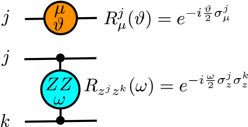
Figure 2.3: Circuit representation of the elementary gates in the conventional model. The top picture indicates a single-qubit rotation while the bottom one indicates the two-qubit Ising gate. Any quantum algorithm can be represented by a circuit composed of these elementary gates.

Every (logical) state of the quantum register has associated a mathematical object denoted as bra in the following way

$$|{n}\rangle\leftrightarrow\langle{n}|,$$ (2.6)

and can be linearly extended for a general state $|{\psi}\rangle$ by conjugation as

$$\sum_{n}a_{n}|{n}\rangle\leftrightarrow\sum_{n}a_{n}^{*}\langle{n}|,$$ (2.7)

where $a_{n}^{*}$ denotes the complex conjugate of $a_{n}$. The product between a logical bra and a logical ket defines the inner-product in the associated Hilbert space given by

$$\langle{m}||{n}\rangle=\langle m|{n}\rangle=\delta_{mn},$$ (2.8)

with $\delta_{mn}$ being the Kronecker delta. In this vectorial space, two vectors (states) $|{\psi}\rangle$ and $|{\phi}\rangle$ are orthogonal if their overlap, that is, their inner product $\langle\psi|{\phi}\rangle$ given by Eq. 2.8, vanishes. Moreover, the bra-ket notation allows one to represent every (Pauli) operator. For example, the single qubit flip operator $\sigma_{x}$ is represented as $\sigma_{x}=|{0}\rangle\langle{1}|+|{1}\rangle\langle{0}|$. This notation is very useful when computing, for example, expectation values.

A measurement is defined as the action that gives some classical information about the state of the quantum register. In quantum mechanics, a measurement is considered to be a probabilistic process that collapses the actual quantum state of the system [Per98]. For example, a measurement of the polarization in the logical basis of every qubit (i.e., the measurement of the observables $\sigma_{z}^{j}$) when the state of the register is $|{\psi}\rangle=\sum_{n}a_{n}|{n}\rangle$, projects it onto a certain logical state $|{m}\rangle$ with probability $|a_{m}|^{2}$ (Bohm’s rule). This is a von Neumann measurement. In particular, in a general von Neumann measurement of an observable $\hat{M}$ ($\equiv\hat{M}^{\dagger}$), the probability $p_{m}$ that the outcome $m$ is obtained, where $m$ is one possible eigenvalue of $\hat{M}$, is given by [NC00]

$$p_{m}=\langle{\psi}|\hat{M}^{\dagger}_{m}\hat{M}_{m}|{\psi}\rangle,$$ (2.9)

where $\hat{M}_{m}$ is the projector onto the subspace of states with quantum number $m$. Moreover, if $m$ is the actual outcome, the state after the measurement is given by

$$|{\psi^{\prime}}\rangle=\frac{\hat{M}_{m}}{\sqrt{\langle{\psi}|\hat{M}_{m}^{\dagger}\hat{M}_{m}|{\psi}\rangle}}|{\psi}\rangle.$$ (2.10)

For example, when measuring the operator $\sigma_{x}$ for a single qubit state $|{0}\rangle$, the two possible outcomes are $m=\pm 1$ (i.e., the eigenvalues of $\sigma_{x}$). Since $|{0}\rangle=\frac{1}{\sqrt{2}}[|{+}\rangle+|{-}\rangle]$, the corresponding probabilities are

$$p_{1}=p_{-1}=1/2,$$ (2.11)

and if the outcome is $+1$ ($-1$), the state is projected onto $|{+}\rangle$ ($|{-}\rangle$). Therefore, to obtain accurate information about the actual state of the quantum system, one needs to prepare many copies of the state and perform many different measurements.

The expectation value of a measurement outcome is the expectation of the outcomes of many measurement repetitions. It can also be expressed in the bra-ket notation. If the state of the quantum system is $|{\psi}\rangle$, the expectation value of $\hat{M}$ is given by

$$\langle\hat{M}\rangle=\langle{\psi}|\hat{M}|{\psi}\rangle.$$ (2.12)

In the conventional model, any observable $\hat{M}$ can be written as a combination (sums and/or products) of the identity and Pauli operators. Therefore, if $|{\psi}\rangle$ is known, the expectation $\langle\hat{M}\rangle$ can be algebraically computed by obtaining first the state $\hat{M}|{\psi}\rangle$, and by projecting it onto the bra $\langle{\psi}|$ using the inner-product relations of Eq. 2.8. For example, if a two-qubit state is given by $|{\psi}\rangle=\frac{1}{\sqrt{2}}[|{0_{1}0_{2}}\rangle+|{1_{1}1_{2}}\rangle]$, then

$$\langle{\psi}|\sigma_{z}^{1}|{\psi}\rangle=\frac{1}{2}\left(\langle{0_{1}0_{2}}|+\langle{1_{1}1_{2}}|\right)\left(|{0_{1}0_{2}}\rangle-|{1_{1}1_{2}}\rangle\right)=0,$$ (2.13)

and

$$\langle{\psi}|\sigma_{x}^{1}\sigma_{x}^{2}|{\psi}\rangle=\frac{1}{2}\left(\langle{0_{1}0_{2}}|+\langle{1_{1}1_{2}}|\right)\left(|{1_{1}1_{2}}\rangle+|{0_{1}0_{2}}\rangle\right)=1.$$ (2.14)

Equations 2.13 and 2.14 have been obtained by noticing that $\sigma_{z}^{1}|{1_{1}1_{2}}\rangle=-|{1_{1}1_{2}}\rangle$, $\sigma_{x}^{1}\sigma_{x}^{2}|{0_{1}0_{2}}\rangle=|{1_{1}1_{2}}\rangle$, and $\sigma_{x}^{1}\sigma_{x}^{2}|{1_{1}1_{2}}\rangle=|{0_{1}0_{2}}\rangle$, together with Eq. 2.8.

Nevertheless, certain quantum computations and QSs are done by evolving mixed states instead of pure states. A quantum register in a probabilistic mixture of pure states can be described in the bra-ket notation by a density matrix $\rho=\sum_{s}p_{s}\rho_{s}$, with $\rho_{s}=|{\psi_{s}}\rangle\langle{\psi_{s}}|$ representing the quantum register being in the pure state $|{\psi_{s}}\rangle$, with probability $p_{s}$ ($\sum_{s}p_{s}=1;p_{s}\geq 0$). Equivalently, every density operator $\rho$ can also be written as a combination (sums and/or products) of the Pauli operators $\sigma_{\alpha}^{j}$ ($\alpha=x,y,z$) and the identity operator ${\mathchoice{\rm 1\mskip-4.0mul}{\rm 1\mskip-4.0mul}{\rm 1\mskip-4.5mul}{\rm 1\mskip-5.0mul}}$. These mixed states are useful when performing quantum computation with devices such as the NMR QC, where the state of the quantum register is approximated by the average state of an ensemble of molecules at room temperature; that is, an extremely mixed state. The expectation value of a measurement outcome over a mixed state is given by

$$\langle\hat{M}\rangle={\sf Tr}(\rho\hat{M}),$$ (2.15)

where $\hat{M}$ is the measured observable, $\rho$ the density operator of the mixed state, and ${\sf Tr}$ denotes the trace.

In brief, the conventional model allows one to describe every step in a QS by means of Pauli operators. The idea is to represent any quantum algorithm (QA) as a circuit composed of elementary single and two-qubit gates, together with the measurement process. The complexity of a QA is then determined by the amount of resources required, given by the number of qubits needed, the number of universal single and two-qubit operations (Fig. 2.3), and the number of measurements needed to obtain an accurate result (e.g., the number of times that the algorithm needs to be performed). For this purpose, a procedure to decompose an arbitrary operation in terms of elementary gates has to be explained. In the following subsection, I present some useful techniques and examples.

2.1.2 Hamiltonian Evolutions

When simulating a physical system on a QC it is necessary, in general, to perform a Hamiltonian (unitary) evolution to the quantum register [OGK01, SOG02], of the form

$$U(t)=e^{-iHt}={\mathchoice{\rm 1\mskip-4.0mul}{\rm 1\mskip-4.0mul}{\rm 1\mskip-4.5mul}{\rm 1\mskip-5.0mul}}-iHt+\frac{1}{2}(-iHt)^{2}+\cdots,$$ (2.16)

where $H=H^{\dagger}$ is a physical Hamiltonian and $t$ is a real parameter (e.g., time). A common $H$ is given by

$$H=H_{x}+H_{y}=\bar{\alpha}\ \sigma_{x}^{1}\left(\prod\limits_{i=2}^{j-1}\sigma_{z}^{i}\right)\sigma^{j}_{x}+\bar{\beta}\ \sigma_{y}^{1}\left(\prod\limits_{i=2}^{j-1}\sigma_{z}^{i}\right)\sigma^{j}_{y}\ ,$$ (2.17)

where $\bar{\alpha}$ and $\bar{\beta}$ are real numbers. From Eqs. 2.4 and 2.5 one obtains $[H_{x},H_{y}]=0$, and therefore, $U(t)=e^{-iH_{x}t}e^{-iH_{y}t}$.

To decompose $U(t)$ into single and two-qubit operations, the following steps can be taken. First, the unitary operator

$$U_{1}=e^{i\frac{\pi}{4}\sigma_{y}^{1}}=\frac{1}{\sqrt{2}}\left[{{\mathchoice{\rm 1\mskip-4.0mul}{\rm 1\mskip-4.0mul}{\rm 1\mskip-4.5mul}{\rm 1\mskip-5.0mul}}}+i\sigma_{y}^{1}\right]$$ (2.18)

takes $\sigma_{z}^{1}\rightarrow\sigma_{x}^{1}$, i.e., $U_{1}^{\dagger}\sigma_{z}^{1}U_{1}=\sigma_{x}^{1}$, so $U_{1}^{\dagger}e^{i{\bar{\alpha}}\sigma_{z}^{1}}U_{1}=e^{i{\bar{\alpha}}\sigma_{x}^{1}}$. Second, the operator

$$U_{2}=e^{i{\pi\over 4}\sigma_{z}^{1}\sigma_{z}^{2}}=\frac{1}{\sqrt{2}}\left[{{\mathchoice{\rm 1\mskip-4.0mul}{\rm 1\mskip-4.0mul}{\rm 1\mskip-4.5mul}{\rm 1\mskip-5.0mul}}}+i\sigma_{z}^{1}\sigma_{z}^{2}\right]$$

takes $\sigma^{1}_{x}\rightarrow\sigma^{1}_{y}\sigma^{2}_{z}$, so $U_{2}^{\dagger}e^{i{\bar{\alpha}}\sigma_{x}^{1}}U_{2}=e^{i{\bar{\alpha}}\sigma_{y}^{1}\sigma_{z}^{2}}$. Then,

$$U_{3}=e^{i{\pi\over 4}\sigma_{z}^{1}\sigma_{z}^{3}}$$

takes $\sigma^{1}_{y}\sigma^{2}_{z}\rightarrow-\sigma^{1}_{x}\sigma^{2}_{z}\sigma^{3}_{z}$. By successively similar steps the required string of operators can be easily built: $\sigma_{x}^{1}\sigma_{z}^{2}\cdots\sigma_{z}^{j-1}\sigma^{j}_{x}$ and also $\exp[i{\bar{\alpha}}\sigma_{x}^{1}\sigma_{z}^{2}\cdots\sigma_{z}^{j-1}\sigma^{j}_{x}]$ (up to a global irrelevant phase):

$$U_{k}^{\dagger}\cdots U_{2}^{\dagger}U_{1}^{\dagger}e^{i{\bar{\alpha}}\sigma_{z}^{1}}U_{1}U_{2}\cdots U_{k}=\exp\left[i{\bar{\alpha}}\sigma_{x}^{1}\sigma_{z}^{2}\cdots\sigma_{z}^{j-1}\sigma^{j}_{x}\right]\$$ (2.19)

where the integer $k$ scales linearly with $j$. The evolution $e^{-iH_{y}t}$ can be decomposed similarly so $U(t)$ is decomposed as the product of both decompositions.

2.1.3 Controlled Operations

Alternatively, one can use the well known Controlled-Not, or CNOT, gate instead of the two-qubit Ising gate. Its action on a pair of qubits (1 and 2) is

$$\mbox{CNOT}\left\{\begin{array}[]{c}|{0_{1}0_{2}}\rangle\rightarrow|{0_{1}0_{2}}\rangle\ ,\ \ |{0_{1}1_{2}}\rangle\rightarrow|{0_{1}1_{2}}\rangle\ ,\\ |{1_{1}0_{2}}\rangle\rightarrow|{1_{1}1_{2}}\rangle\ ,\ \ |{1_{1}1_{2}}\rangle\rightarrow|{1_{1}0_{2}}\rangle\ .\\ \end{array}\right.$$

Here, qubit 1 is the control qubit (the controlled operation on its state $|{1_{1}}\rangle$ is represented by a solid circle in Fig. 2.4). If the state of qubit 1 is $|{0_{1}}\rangle$ nothing happens (identity operation) but if its state is $|{1_{1}}\rangle$, the state of qubit 2 is flipped. The decomposition of the CNOT unitary operation into single and two-qubit operations is

$$\mbox{CNOT: }e^{i\frac{\pi}{4}}e^{-i\frac{\pi}{4}\sigma_{z}^{1}}e^{-i\frac{\pi}{4}\sigma_{x}^{2}}e^{i\frac{\pi}{4}\sigma_{z}^{1}\sigma_{x}^{2}},$$ (2.20)

which was obtained by noticing that $ie^{-i\frac{\pi}{2}\sigma_{x}^{2}}\equiv\sigma_{x}^{2}$, i.e., the spin-flip operator acting on qubit 2 (Eq. 2.1):

$$\sigma_{x}^{2}\left\{\matrix{|{\phi_{1}0_{2}}\rangle\rightarrow|{s_{1}1_{2}}\rangle\ ,\cr|{\phi_{1}1_{2}}\rangle\rightarrow|{s_{1}0_{2}}\rangle\ .}\right.$$ (2.21)

By using the techniques described in Sec. 2.1.2, the CNOT operation in terms of single and two-qubit Ising gates is

$$\mbox{CNOT: }e^{i\frac{\pi}{4}}e^{-i\frac{\pi}{4}\sigma_{z}^{1}}e^{-i\frac{\pi}{4}\sigma_{x}^{2}}e^{i\frac{\pi}{4}\sigma_{y}^{2}}e^{-i\frac{\pi}{4}\sigma_{z}^{1}\sigma_{z}^{2}}e^{-i\frac{\pi}{4}\sigma_{y}^{2}}\ .$$ (2.22)

The circuit representation of this decomposition is shown in Fig. 2.4. Five elementary single and two-qubit Ising gates are required to perform the CNOT gate.

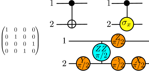
Figure 2.4: CNOT gate decomposition and its matrix representation. The control qubit is 1. Note that the last circuit realizes the CNOT matrix operation up to a global phase $e^{-i\frac{\pi}{4}}$.

These results can be extended to other controlled unitary operations like the CU operation defined as

$$\mbox{CU: }|{0}\rangle_{\sf a}\langle{0}|\otimes{\mathchoice{\rm 1\mskip-4.0mul}{\rm 1\mskip-4.0mul}{\rm 1\mskip-4.5mul}{\rm 1\mskip-5.0mul}}_{s}+|{1}\rangle_{\sf a}\langle{1}|\otimes U_{s}.$$ (2.23)

The unitary operation above performs the transformation $U_{s}$ (also unitary) over a set of qubits $s$ if the state of the control qubit ${\sf a}$ is $|{1}\rangle$, and does not act otherwise. For the transformation $U_{s}\equiv U(t)=e^{-i\hat{Q}t}$, with $\hat{Q}=\hat{Q}^{\dagger}$, the operational representation of the CU gate is

$$U(t/2)U(t/2)^{-\sigma_{z}^{\sf a}},$$ (2.24)

where $U(t/2)^{-\sigma_{z}^{\sf a}}\equiv e^{i\hat{Q}\otimes\sigma_{z}^{\sf a}}$ [Fig. 2.5(a)]. Equivalently, one can define another controlled operation, CU’, on the state $|{0}\rangle_{\sf a}$ [Fig. 2.5(b)]: $U(t/2)U(t/2)^{\sigma_{z}^{\sf a}}$.

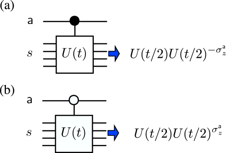
Figure 2.5: (a) CU operation with the state of the control qubit ${\sf a}$ being in $|{1}\rangle_{\sf a}$ and (b) CU’ operation controlled with the state $|{0}\rangle_{\sf a}$.

Controlled operations are widely used in quantum algorithms. In general, their decomposition into single and two-qubit gates require a large number of these elementary operations, so they should be avoided when possible.

2.2 Deterministic Quantum Algorithms

In a QS, a QC performs certain tasks which are expected to give some information about the physical system being simulated. These tasks are communicated by means of a program or quantum algorithm (QA), which can be schematically represented as a quantum circuit. In this section, I present a particular type of QA that can be used to obtain relevant properties of a quantum physical system $s$, using the conventional model (Sec. 2.1). Nevertheless, the same techniques can be used to simulate physical systems with other particle statistics (e.g., fermionic or bosonic systems), if they can be described by Pauli operators after an algebraic mapping.

A deterministic QA is based on three different steps: i) the preparation of a pure initial state, ii) its evolution, and iii) the measurement of certain property of the evolved state, in which the result of the algorithm is encoded. To preserve the features of the quantum world, the evolution step is performed through a unitary operation and the measurement step is described by a certain observable (i.e., Hermitian operator). Here, I present only the class of QAs that allows one to determine, in a register of $N$ qubits, physical correlation functions of the form

$$G=\langle{\phi}|\hat{W}_{s}|{\phi}\rangle,$$ (2.25)

where $\hat{W}_{s}$ is a unitary (reversible) operator associated to the system to be simulated; that is, $\hat{W}_{s}\hat{W}_{s}^{\dagger}={\mathchoice{\rm 1\mskip-4.0mul}{\rm 1\mskip-4.0mul}{\rm 1\mskip-4.5mul}{\rm 1\mskip-5.0mul}}$ ($s$ refers to the system).

Indirect measurement techniques can be used to obtain such correlation functions on a QC. In addition to the qubits used to represent the physical system $s$ to be simulated (i.e., the qubits-system) extra qubits, called ancillas, are required. These ancillas constitute the probes that contain information about the qubits-system. In the following section I describe different measurement techniques.

2.2.1 One-Ancilla Qubit Measurement Processes

In this case a single ancilla qubit allows one to obtain the correlation functions of Eq. 2.25, with $\hat{W}_{s}=U^{\dagger}V$, and $U$, $V$ unitary operators acting on $s$ [OGK01]. For this purpose, the ancilla qubit ${\sf a}$ is first initialized in the state $|{+}\rangle_{\sf a}=\frac{1}{\sqrt{2}}(|{0}\rangle_{\sf a}+|{1}\rangle_{\sf a})$ by applying, for example, the unitary Hadamard gate to the state $|{0}\rangle_{\sf a}$. Second, one makes it interact with the qubits-system, initially in certain pure state $|{\phi}\rangle$, through two controlled unitary operations $\tilde{V}$ and $\tilde{U}$, associated to the $V$ and $U$ operations, respectively. The first operation $\tilde{V}$ evolves the system by $V$ if the ancilla is in the state $|{1}\rangle$: $\tilde{V}=|{0}\rangle_{\sf a}\langle{0}|\otimes{\mathchoice{\rm 1\mskip-4.0mul}{\rm 1\mskip-4.0mul}{\rm 1\mskip-4.5mul}{\rm 1\mskip-5.0mul}}_{s}+|{1}\rangle_{\sf a}\langle{1}|\otimes V$. The second operation $\tilde{U}$ evolves the system by $U$ if the ancilla state is $|{0}\rangle$: $\tilde{U}=|{0}\rangle_{\sf a}\langle{0}|\otimes U+|{1}\rangle_{\sf a}\langle{1}|\otimes{\mathchoice{\rm 1\mskip-4.0mul}{\rm 1\mskip-4.0mul}{\rm 1\mskip-4.5mul}{\rm 1\mskip-5.0mul}}_{s}$. Notice that $\tilde{V}$ and $\tilde{U}$ are reversible and commute with each other.

After such evolution, the final state of the quantum register, $|{\psi_{f}}\rangle$, is

$$|{\psi_{f}}\rangle=\tilde{V}\tilde{U}|{+}\rangle_{\sf a}|{\phi}\rangle=\frac{1}{\sqrt{2}}\left[|{0}\rangle_{\sf a}\otimes U|{\phi}\rangle+|{1}\rangle_{\sf a}\otimes V|{\phi}\rangle\right].$$ (2.26)

Interestingly, the expectation value of the Pauli operator $2\sigma_{+}^{\sf a}=\sigma_{x}^{\sf a}+i\sigma_{y}^{\sf a}$ associated with the ancilla qubit, in this state, gives the desired correlation function:

$$G=\langle\psi_{f}|\sigma_{x}^{\sf a}+i\sigma_{y}^{\sf a}|\psi_{f}\rangle,$$ (2.27)

where I have used the orthogonality property (Sec. 2.1.1), that is, $\langle 0|{1}\rangle_{\sf a}=\langle 1|{0}\rangle_{\sf a}=0$, $\langle 0|{0}\rangle_{\sf a}=\langle 1|{1}\rangle_{\sf a}=1$, and the action of the operators $\sigma_{\mu}^{\sf a}$ over the state of the ancilla qubit given by Eq. 2.1. The corresponding circuit for this quantum algorithm is shown in Fig. 2.6. Due to the probabilistic nature of quantum measurements, the desired expectation value is obtained with variance ${\cal O}(1)$ for each instance. That is, in order to get an accurate value for $\langle 2\sigma_{+}^{\sf a}\rangle$, repetition must be used to reduce the variance below what is required (Sec. 2.1.1).

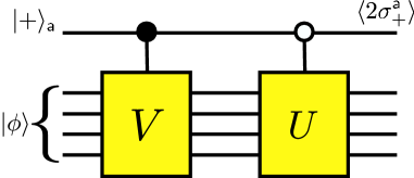
Figure 2.6: Quantum algorithm for the evaluation of the correlation $G=\langle{\phi}|U^{\dagger}V|{\phi}\rangle$.

Nevertheless, sometimes it is necessary to compute the expectation value of an operator $\hat{W}$ of the form

$$\hat{W}=\sum\limits_{i=1}^{M}a_{i}\ U^{\dagger}_{i}V_{i}\ ,$$ (2.28)

where $U_{i}$ and $V_{i}$ are unitary operators, $a_{i}\geq 0\in\mathbb{R}$ (with no loss of generality). In principle, this expectation value can be computed by preparing $M$ different circuits as the one represented in Fig. 2.6, such that each algorithm computes $\langle U^{\dagger}_{i}V_{i}\rangle$. However, in most practical cases, the preparation of the initial state $|{\phi}\rangle$ is a very difficult task. This difficulty can then be reduced by using a particular QA that requires only one circuit, but with $L$ ancilla qubits, where $L=J+1$ and $J\geq\log_{2}M$. Such QA has been described in Ref. [SOG02]. The idea is to extend the results described above using controlled operations with respect to different ancilla qubits.

2.2.2 Quantum Algorithms and Quantum Simulations

Based on the indirect-measurement methods described in Sec. 2.2.1, I now present certain QAs for QSs. These are useful for obtaining relevant properties of quantum systems, like the evaluation of the correlation function

$$G(t)=\langle\phi|T^{\dagger}A^{\dagger}_{i}TB_{j}|\phi\rangle.$$ (2.29)

Here, $A_{i}$ and $B_{j}$ are unitary operators (any operator can be decomposed in a unitary operator basis as $A=\sum\limits_{i}\alpha_{i}A_{i}$, $B=\sum\limits_{j}\beta_{j}B_{j}$), $T=e^{-iHt}$ is the time evolution operator of a time-independent Hamiltonian $H$ associated to the physical system to be simulated, and $|{\phi}\rangle$ is a particular state of the physical system. Notice that Eq. 2.29 is a particular case of Eq. 2.25. In particular, the evaluation of spatial correlation functions can be obtained by replacing the evolution operator $T$ by the space translation operator.

The quantum circuit for the evaluation of $G(t)$ is shown in Fig. 2.7. It is equivalent to the one shown in Fig. 2.6 by choosing $U^{\dagger}=T^{\dagger}A_{i}$ and $V=TB_{j}$. This particular selection allows one to reduce the complexity of the problem in the sense that the operation $T$ need not to be controlled by the state of the ancilla qubit ([SOG02]). As mentioned in Sec. 2.1.3, controlled operations require a large number of elementary gates, so they must be avoided when possible.

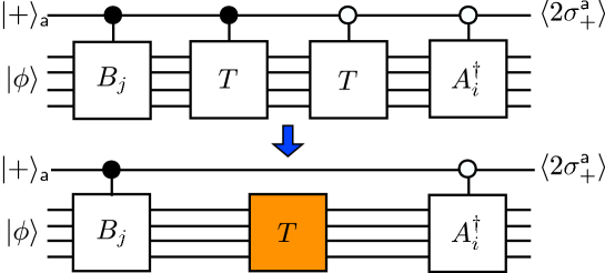
Figure 2.7: Quantum algorithm for the computation of spatial and time-correlation functions. In this case, $\langle 2\sigma_{+}^{\sf a}\rangle=\langle{\phi}|T^{\dagger}A^{\dagger}_{i}TB_{j}|{\phi}\rangle$. Notice the simplification achieved by reducing the controlled-T operations. The same convention of Fig. 2.6 has been used.

In brief, the computation of $G(t)$ is performed as follows: First, the ancilla qubit ${\sf a}$ is prepared in the state $|{+}\rangle_{\sf a}$, and the system is prepared in the state $|{\phi}\rangle$. Second, a controlled evolution on the state $|{1}\rangle_{\sf a}$, given by $\mbox{C-B}=|{0}\rangle_{\sf a}\langle 0|\otimes{\mathchoice{\rm 1\mskip-4.0mul}{\rm 1\mskip-4.0mul}{\rm 1\mskip-4.5mul}{\rm 1\mskip-5.0mul}}_{s}+|{1}\rangle_{\sf a}\langle 1|\otimes B_{j}$, is performed. Third, the time evolution $T$ is performed. Fourth, a controlled evolution on the state $|{0}\rangle_{\sf a}$, given by $\mbox{C-A}=|{0}\rangle_{\sf a}\langle 0|\otimes A_{i}+|{1}\rangle_{\sf a}\langle 1|\otimes{\mathchoice{\rm 1\mskip-4.0mul}{\rm 1\mskip-4.0mul}{\rm 1\mskip-4.5mul}{\rm 1\mskip-5.0mul}}_{s}$, is performed. Finally the observable $\langle 2\sigma_{+}^{\sf a}\rangle=\langle\sigma_{x}^{\sf a}+i\sigma_{y}^{\sf a}\rangle=G(t)$ is measured.

Sometimes one is interested in obtaining the spectrum (eigenvalues) of a given observable $\hat{Q}$ ( Hermitian operator), associated with some physical property of the system to be simulated. Techniques for getting spectral information can be used on the quantum Fourier transform [Kit95, CEM98] and can be applied to physical problems [AL99]. Nevertheless, the idea here is to use the methods developed in Sec. 2.2.1.

For some Hermitian operator $\hat{Q}$, such as the Hamiltonian $H$ of the system to be simulated, a common type of problem is the computation of its eigenvalues or, at least, the lowest eigenvalue (related, for example, to the ground state of the system). For this purpose, the qubits-system needs to be initialized in a certain state $|{\phi}\rangle$, that has a non-zero overlap with the eigenstates corresponding to the eigenvalues that need to be computed. Such a state can always be decomposed as a linear combination of eigenstates of $\hat{Q}$,

$$|{\phi}\rangle=\sum_{n}\gamma_{n}\ |{\psi_{n}}\rangle,$$ (2.30)

where $\gamma_{n}$ are complex coefficients, $|{\psi_{n}}\rangle$ are the eigenstates of $\hat{Q}$, and $\lambda_{n}$ the corresponding eigenvalues. If interested in computing $\lambda_{m}$, it is then required that $|\gamma_{m}|\neq 0$ in Eq. 2.30.

For this purpose, the correlation function

$$S(t)=\langle{\phi}|U(t)|{\phi}\rangle,$$ (2.31)

with $U(t)=e^{-i\hat{Q}t}$, needs to be computed for different values of the real parameter $t$ (usually related with time). For a particular $t$, the measurement of $S(t)$ can be performed using the one-ancilla method (Sec. 2.2.1) as follows. First, the initial state $|{+}\rangle_{\sf a}\otimes|{\phi}\rangle$ is prepared. Second, the unitary evolution $\exp[i\hat{Q}\sigma_{z}^{\sf a}t/2]$ is performed. Finally, the expectation $\langle 2\sigma_{+}^{\sf a}\rangle=S(t)$ is measured. The circuit representation of this QA is shown in Fig. 2.8. It is equivalent to the one shown in Fig. 2.6 by replacing $U^{\dagger}=V=e^{-i\hat{Q}t/2}$.

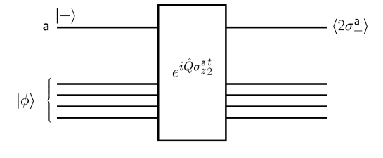
Figure 2.8: Quantum algorithm for the computation of the spectrum of an observable $\hat{Q}$. In this case, $\langle 2\sigma_{+}^{\sf a}\rangle=\langle{\phi}|e^{-i\hat{Q}t}|{\phi}\rangle$.

For a particular value of $t$, the function $S(t)$ is

$$S(t)=\sum_{n}|\gamma_{n}|^{2}\ e^{-i{\lambda}_{n}t}.$$ (2.32)

Then, the eigenvalues $\lambda_{n}$ can be obtained by performing a classical Fourier transform to Eq. 2.32 (i.e., $\tilde{S}(\lambda)=\int S(t)e^{i\lambda t}dt$)

$$\tilde{S}(\lambda)=\sum_{n}2\pi|\gamma_{n}|^{2}{\delta}({\lambda}-{\lambda}_{n})\ .$$ (2.33)

However, $S(t)$ is only obtained for a discrete set of values of $t$. It is needed, instead, to calculate the corresponding discrete Fourier transform (see Appendix A) to obtain information about the $\lambda_{n}$’s.

2.3 Quantum Simulations of Quantum Physics

In the most general case, a QS requires the simulation of systems with diverse degrees of freedom, like fermions, anyons, bosons, etc. The associated Hilbert spaces (space of states) differ from the one defined for the conventional model. For example, in the case of fermionic systems, fermionic states are governed by Pauli’s exclusion principle. Then, at most a single spinless (or two spin-1/2) fermion can occupy a certain (atomic) quantum state at the same time. Therefore, all the features associated with the physical system to be simulated must be preserved when transforming its operators to the operators describing the computational model of the QC.

In this section, I present isomorphic mappings that allow one to simulate arbitrary quantum systems, regardless of their particle statistics, by using the QAs defined for the conventional model (Sec. 2.2). Fortunately, such mappings can be easily performed without breaking the efficiency of a QA.

2.3.1 Simulations of Fermionic Systems

The systems considered here consist mainly of a lattice with $N$ modes (sites), where spinless fermions can hop between sites. These results can be easily extended for the case of spin-1/2 fermions or higher spin fermions.

In the second quantization representation, the (spinless) fermionic operators $c^{\dagger}_{j}$ and $c^{\;}_{j}$ are defined as the creation and annihilation operators of a fermion in the $j$-th mode ($j=1,\cdots,N$), respectively. Due to the Pauli’s exclusion principle and the antisymmetric nature of the fermionic wave function under the permutation of two fermions, the fermionic algebra is given by the following anticommutation relations

$$\{c_{i},c_{j}\}=0,\mbox{ }\{c^{\dagger}_{i},c_{j}\}=\delta_{ij}$$ (2.34)

where $\{,\}$ denotes the anticommutator (i.e., $\{A,B\}=AB+BA$).

The Jordan-Wigner transformation [JW28] is the isomorphic mapping that allows the description of a fermionic system by the conventional model. It is performed in the following way:

$$c_{j}\rightarrow\left(\prod\limits_{l=1}^{j-1}-\sigma_{z}^{l}\right)\sigma_{-}^{j},$$ (2.35)

$$c^{\dagger}_{j}\rightarrow\left(\prod\limits_{l=1}^{j-1}-\sigma_{z}^{l}\right)\sigma_{+}^{j},$$ (2.36)

where the Pauli operators $\sigma_{\mu}^{i}$ were previously introduced in Sec 2.1. If these operators satisfy the $\mathfrak{su}(2)$ commutation relations (Eqs. 2.4 and 2.5), the operators $c^{\dagger}_{j}$ and $c^{\;}_{j}$ obey the anticommutation relations of Eqs. 2.34. This is an isomorphic mapping between operator algebras and is independent of the Hamiltonian of the fermionic system to be simulated.

Different Hamiltonians establish different connections (connectivity) between fermionic modes. Historically, Eqs. 2.35 and 2.36 correspond to lattices in one space dimension. Nevertheless, it is also valid for lattice systems in any dimension, when the set of modes $j$ is countable. In particular, the set of all ordered $p$-tuples of integers can be placed in one-to-one correspondence with the set of integers. For example, the simulation of a two dimensional fermionic lattice system can be done by re-mapping each mode $(l,m)$ into a new set of modes as $j=m+(l-1)N_{x}$, where $[l=1\cdots N_{y}]$ and $[m=1\cdots N_{x}]$ are integer numbers that refer to the position of a site in the lattice, and $N_{x}$ and $N_{y}$ are the number of sites (modes) in the $x$ and $y$ direction, respectively.

In order to compute physical properties of a fermionic system on a QC described by the conventional model, every step of the quantum simulation has to be expressed in terms of Pauli operators. For a (spinless) fermionic system with $N$ modes, a QC must contain, besides the ancilla qubit ${\sf a}$, $N$ qubits to represent the system. In the following, I describe how certain fermionic initial states can be prepared and how they can be evolved under a particular fermionic Hamiltonian evolution.

Preparation of Initial Fermionic States

Associated to each fermionic mode, there are two levels which correspond to the mode being empty or being occupied by a spinless fermion. The state-state mapping is then trivial. Basically, the logical state $|{1_{j}}\rangle$ is associated to the $j$th mode if it is empty, and the logical state $|{0_{j}}\rangle$ (up to a phase) is associated if the $j$th mode is occupied. In this way, the vacuum or no-fermion state $|{\sf vac}\rangle$, which satisfies $c_{j}|{{\sf vac}}\rangle=0\mbox{ }\forall j$, is mapped to the logical $N$-qubit state $|{1_{1}1_{2}\cdots 1_{N}}\rangle$.

However, when simulating a fermionic system, more complex states need to be prepared. A general state $|{\psi}\rangle$ of $N_{e}$ fermions is a linear combination of Slater determinants (i.e., fermionic product states),

$$|{\psi}\rangle=\sum\limits_{\alpha=1}^{L}g_{\alpha}\ |{\phi_{\alpha}}\rangle,$$ (2.37)

where the Slater determinants $|{\phi_{\alpha}}\rangle$ are

$$|{\phi_{\alpha}}\rangle=\prod\limits_{j=1}^{N_{e}}c^{\dagger}_{j}\ |{\sf vac}\rangle.$$ (2.38)

Due to the anticommutation relations of Eqs. 2.34, the fermionic operators satisfy

$$c^{\dagger}_{i}c^{\dagger}_{j}=-c^{\dagger}_{j}c^{\dagger}_{i}\mbox{ if }i\neq j,$$ (2.39)

implying that the Slater determinants $|{\phi_{\alpha}}\rangle$ are antisymmetric wave functions under the permutation of an even number of fermions.

Every state $|{\phi_{\alpha}}\rangle$ can be prepared on a QC made of qubits, by noticing that the quantum gate (i.e., unitary operator)

$$U_{m}=e^{i\frac{\pi}{2}(c^{\;}_{m}+c^{\dagger}_{m})}$$ (2.40)

creates a particle in the $m$-th mode when acting on the vacuum state. In other words, $U_{m}|{{\sf vac}}\rangle=e^{i\frac{\pi}{2}}c^{\dagger}_{m}|{\sf vac}\rangle$. Then, making use of the Jordan-Wigner transformation (Eqs. 2.35 and 2.36), the operators $U_{m}$ in the spin language are

$$\tilde{U}_{m}=e^{i\frac{\pi}{2}\sigma_{x}^{m}\prod\limits_{j=1}^{m-1}-\sigma_{z}^{j}}.$$ (2.41)

The operators $\tilde{U}_{m}$ can easily be decomposed into elementary single and two-qubit gates as described in Sec. 2.1.2. The successive application of $N_{e}$ similar unitary operators to the state $|{1_{1}1_{2}\cdots 1_{N}}\rangle$ generates the mapped state $|{\phi_{\alpha}}\rangle$, up to an irrelevant global phase.

The general fermionic state of Eq. 2.37 can be prepared by using $L$ ancilla qubits, performing unitary controlled-$\tilde{U}_{m}$ evolutions on the state of the ancillas, and finally, performing a measurement (projecting) on the ancillas. For example, if one is interested in preparing the state $|{\psi}\rangle=\frac{1}{\sqrt{2}}[|{\phi_{1}}\rangle+|{\phi_{2}}\rangle]$, one needs to add an extra ancilla to the system. This ancilla is prepared in the state $|{+}\rangle_{\sf a}$ and a controlled evolution to obtain the state $\frac{1}{\sqrt{2}}[|{0}\rangle_{\sf a}\otimes|{\phi_{1}}\rangle+|{1}\rangle_{\sf a}\otimes|{\phi_{2}}\rangle]$, is performed later. If the Hadamard gate is applied to the ancilla, this state evolves into

$$|{0}\rangle_{\sf a}\otimes\frac{1}{\sqrt{2}}[|{\phi_{1}}\rangle+|{\phi_{2}}\rangle]+|{1}\rangle_{\sf a}\otimes\frac{1}{\sqrt{2}}[|{\phi_{1}}\rangle+|{\phi_{2}}\rangle].$$ (2.42)

Therefore, the ancilla qubit is measured and projected, with probability 1/2, into $|{0}\rangle_{\sf a}$ or $|{1}\rangle_{\sf a}$. If the former is obtained, the desired state is prepared. However, if the ancilla is projected into $|{1}\rangle_{\sf a}$, the whole method needs to be applied again from the begining.

In general, the probability of successful preparation of $|{\psi}\rangle$ (Eq. 2.37) using this method is $1/L$. Then, the order of $L$ trials need to be performed before a successful preparation. A detailed description of this method can be found in Ref. [OGK01].

Nevertheless, an important case consists of the preparation of Slater determinants (product state) $|{\phi_{\beta}}\rangle$ in a different basis mode than the one given before:

$$|{\phi_{\beta}}\rangle=\prod\limits_{j=1}^{N_{e}}d^{\dagger}_{j}\ |{\sf vac}\rangle.$$ (2.43)

The fermionic operators $d^{\dagger}_{j}$’s are sometimes related to the operators $c^{\dagger}_{j}$ through the following canonical transformation

$$\overrightarrow{d}^{\dagger}=e^{i\bar{M}}\overrightarrow{c}^{\dagger},$$ (2.44)

with $\overrightarrow{d}^{\dagger}=(d^{\dagger}_{1},d^{\dagger}_{2},\cdots,d^{\dagger}_{N})$, $\overrightarrow{c}^{\dagger}=(c^{\dagger}_{1},c^{\dagger}_{2},\cdots,c^{\dagger}_{N})$, and $\bar{M}$ being a $N\times N$ Hermitian matrix. (Sometimes the operators $d^{\dagger}$ are combinations of both, the creation and annihilation operators $c^{\dagger}_{i}$ and $c_{i}$.)

Thouless’s theorem states that one Slater determinant evolves into the other as

$$|{\phi_{\beta}}\rangle=U|{\phi_{\alpha}}\rangle,$$ (2.45)

where the unitary fermionic operator

$$U=e^{-i\overrightarrow{c}^{\dagger}\bar{M},\overrightarrow{c}}$$ (2.46)

can be written in terms of Pauli operators using the Jordan-Wigner transformation (Sec.2.3.1), and can also be decomposed into elementary gates as described in Sec. 2.1.2.

In brief, the described fermionic product states can be prepared on a QC described by the conventional model, if the Jordan-Wigner transformation is performed. Interestingly, the preparation can be done efficiently: the number of elementary single-qubit and two-qubit gates required scales polynomially with the system size $N$. In Chap. 4, I present another class of fermionic states that can also be prepared efficiently.

Fermionic Evolutions

The evolution of a quantum state is the second step in the realization of a QA. The goal is to decompose a generic evolution into the elementary gates $R_{\mu}(\vartheta)\mbox{ and }R_{z^{j}z^{k}}(\omega)$ (Sec. 2.1). Sometimes, the evolution step is associated to a Hermitian operator $\tilde{H}$ which is, for example, the Hamiltonian $H$ of the fermionic system to be simulated in terms of Pauli operators after Eqs. 2.35 and 2.36 have been performed. In this case, the corresponding evolution unitary operator is $\tilde{U}(t)=e^{-i\tilde{H}t}$ (i.e, the solution to the Schrödinger’s evolution equation).

In general, a fermionic Hamiltonian can be decomposed as $H=K+V$ ,where $K$ represents the kinetic energy of the fermions and $V$ their potential energy. Usually, $[K,V]\neq 0$ and the decomposition of $\tilde{U}(t)$ in terms of elementary gates is a complicated task. To avoid this difficulty this operator is approximated by, for example, using a first order Trotter decomposition [Suz93]. That is,

$$\tilde{U}(t) = \prod\limits_{g=1}^{\cal N}\tilde{U}(\Delta t),$$ (2.47)

$$\tilde{U}(\Delta t) = e^{i\tilde{H}\Delta t}=e^{i(\tilde{K}+\tilde{V})\Delta t}=e^{i\tilde{K}\Delta t}e^{i\tilde{V}\Delta t}+\mathcal{O}(\Delta t^{2}),$$ (2.48)

where $\tilde{K}$ and $\tilde{V}$ are the terms $K$ and $V$ in Pauli operators, respectively. Therefore, for $\Delta t\rightarrow 0$, $\tilde{U}(\Delta t)\sim e^{i\tilde{K}\Delta t}e^{i\tilde{V}\Delta t}$.

The potential energy $V$ is usually a sum of commuting diagonal terms, and the decomposition of $e^{i\tilde{V}\Delta t}$ into elementary gates is simple. However, the kinetic energy $K$ is usually a sum of noncommuting hopping terms of the form $c^{\dagger}_{j}c^{\;}_{k}+c^{\dagger}_{k}c^{\;}_{j}$ (bilinear fermionic operators), and its decomposition is again approximated. A typical kinetic term $e^{i(c^{\dagger}_{j}c^{\;}_{k}+c^{\dagger}_{k}c^{\;}_{j})\Delta t}$ ($j<k$), when mapped onto the spin language gives

$$e^{-\frac{i}{2}(\sigma_{x}^{j}\sigma_{x}^{k}+\sigma_{y}^{j}\sigma_{y}^{k})\prod\limits_{l=j+1}^{k-1}(-\sigma_{z}^{l})}=e^{-\frac{i}{2}\sigma_{x}^{j}\sigma_{x}^{k}\prod\limits_{l=j+1}^{k-1}(-\sigma_{z}^{l})}e^{-\frac{i}{2}\sigma_{y}^{j}\sigma_{y}^{k}\prod\limits_{l=j+1}^{k-1}(-\sigma_{z}^{l})}.$$ (2.49)

The decomposition of each term on the right hand side of Eq. 2.49 into elementary single and two-qubit gates was previously discussed in Sec. 2.1.2. The amount of elementary gates required depends on the distance $|j-k|$, and scales polynomially with that distance. Moreover, since $H$ represents a physical system, it is a linear combination of a polynomially large (with $N$) amount of fermionic operators. Then, $\tilde{U}(t)$ can be performed efficiently by applying a polynomially large amount of elementary gates. In the same way, the unitary operation $U=e^{-i\overrightarrow{c}^{\dagger}M\overrightarrow{c}}$ of Eq. 2.46 can also be efficiently implemented.

Obviously, the accuracy of approximating $\tilde{U}(t)$ using the Trotter decomposition increases as $\Delta t$ decreases. Then, a large amount of gates might be required to perform the desired evolution with small errors. To overcome this problem, one could use a Trotter approximation of higher order in $\Delta t$ [Suz93]. All these approximation methods do not destroy the efficiency of the QA. Moreover, the evolution step induced by fermionic physical Hamiltonians with higher order products of creation and annihilation operators can also be efficiently implemented using the same techniques.

2.3.2 Simulations of Anyonic Systems

The concepts described in Sec. 2.3.1 can be extended to other and more general particle statistics, namely hard-core anyons [BO01]. These are particles that also obey the Pauli’s exclusion principle: At most one (spinless) anyon can occupy a single mode. Assigned to each mode of the lattice are the creation and annihilation anyonic operators $a^{\dagger}_{j}$ and $a^{\;}_{j}$, respectively. Their commutation relations are given by ($j\leq j^{\prime}$)

$$[a^{\;}_{j},a^{\;}_{j^{\prime}}]_{\theta} = [a^{\dagger}_{j},a^{\dagger}_{j^{\prime}}]_{\theta}=0\ ,$$

$${[}a^{\;}_{j},a^{\dagger}_{j^{\prime}}{]}_{-\theta} = \delta_{jj^{\prime}}(1-(e^{-i\theta}+1)n_{j^{\prime}})\ ,$$ (2.50)

$${[}n_{j},a^{\dagger}_{j^{\prime}}] = \delta_{jj^{\prime}}a^{\dagger}_{j^{\prime}}\ ,$$

where $n_{j^{\prime}}=a^{\dagger}_{j^{\prime}}a^{\;}_{j^{\prime}}$ is the number operator, $[A,B]_{\theta}=AB-e^{i\theta}BA$, and $\theta$ is the statistical angle. In particular, $\theta=\pi$ mod($2\pi$) represents canonical spinless fermions, while $\theta=0$ mod($2\pi$) represents hard-core bosons.

In order to simulate this problem on a QC described by the conventional model, the following isomorphic mapping between algebras can be performed:

$$a^{\dagger}_{j} = \prod\limits_{l<j}\left[\frac{e^{-i\theta}+1}{2}+\frac{e^{-i\theta}-1}{2}\sigma_{z}^{l}\right]\ \sigma_{+}^{j},$$

$$a_{j} = \prod\limits_{l<j}\left[\frac{e^{i\theta}+1}{2}+\frac{e^{i\theta}-1}{2}\sigma_{z}^{l}\right]\ \sigma_{-}^{j},$$ (2.51)

$$n_{j} = \frac{1}{2}(1+\sigma_{z}^{j}),$$

where the Pauli operators $\sigma_{\mu}^{i}$ were introduced in Sec. 2.1.1. Since they satisfy the commutation relations of Eqs. 2.4 and 2.5, the commutation relations for the anyonic operators (Eqs. 2.3.2) are satisfied.

As in the fermionic case (Sec. 2.3.1), an anyonic evolution operator can be written in terms of Pauli operators using Eq. 2.51, and can be decomposed into single and two-qubit elementary gates. Therefore, the same procedure described in the previous section can be followed.

Anyon statistics have fermion and hard-core boson statistics as limiting cases, satisfying always the Pauli’s exclusion principle. In the next section this hard-core condition is relaxed and the important case of canonical bosons is considered.

2.3.3 Simulations of Bosonic Systems

Quantum computation is based on the manipulation of quantum systems that possess a finite number of degrees of freedom (e.g., qubits). From this point of view, the simulation of bosonic systems appears to be impossible, since the non-existence of an exclusion principle implies that the Hilbert space used to represent bosonic quantum states on a lattice is infinite-dimensional; that is, there is no limit to the number of bosons that can occupy a given mode $j$. However, sometimes it is necessary to simulate and study properties such that the use of the complete Hilbert space is unnecessary, and only a finite sub-basis of states is sufficient. This is the case for $N$-mode (e.g., $N$ sites) lattice systems with interactions given by the boson-preserving Hamiltonian

$$H=\sum\limits_{j,j^{\prime}=1}^{N}\alpha_{jj^{\prime}}\ b^{\dagger}_{j}b^{\;}_{j^{\prime}}+\beta_{jj^{\prime}}\ \hat{n}_{j}\hat{n}_{j^{\prime}},$$ (2.52)

where the operators $b^{\dagger}_{j}$ ($b^{\;}_{j}$) create (destroy) a boson at site $j$, and $\hat{n}_{j}=b^{\dagger}_{j}b^{\;}_{j}$ is the number operator; that is

$$b^{\dagger}_{j}|{n_{1},n_{2},\cdots,n_{j},\cdots,n_{N}}\rangle = \sqrt{n_{j}+1}\ |{n_{1},n_{2},\cdots,n_{j}+1,\cdots,n_{N}}\rangle,$$

$$b^{\;}_{j}|{n_{1},n_{2},\cdots,n_{j},\cdots,n_{N}}\rangle = \ \ \ \sqrt{n_{j}}\ \ \ \ \ |{n_{1},n_{2},\cdots,n_{j}-1,\cdots,n_{N}}\rangle,$$

$$\hat{n}_{j}|{n_{1},n_{2},\cdots,n_{j},\cdots,n_{N}}\rangle = \ \ \ \ \ n_{j}\ \ \ \ \ \ |{n_{1},n_{2},\cdots,n_{j},\cdots,n_{N}}\rangle,$$ (2.53)

where the bosonic state $|{n_{1},n_{2},\cdots,n_{j},\cdots,n_{N}}\rangle$ represents a quantum state with $n_{j}$ bosons in the $j$-th mode (site).

The space dimension of the lattice is encoded in the parameters $\alpha_{jj^{\prime}}$ and $\beta_{jj^{\prime}}$ of the Hamiltonian. Since $H$ contains pairs of creation and annihilation operators, the total number of bosons $N_{P}$ in the system is preserved and the idea is to work in this finite sub-basis of states (where the dimension of the associated Hilbert space depends on the magnitude of $N_{P}$).

The corresponding bosonic commutation relations (in an infinite-dimensional Hilbert space) are [CDG98]

$$[b_{j},b_{j^{\prime}}]=0,[b_{j},b^{\dagger}_{j^{\prime}}]=\delta_{jj^{\prime}}.$$ (2.54)

However, if the operators $b^{\dagger}_{j}$ are restricted to the finite basis of states represented by $\{|{n_{1},n_{2},\cdots,n_{N}}\rangle$ with $\max(n_{i})=N_{P}\}$, that is, $N_{P}$ is the maximum number of bosons per site, they acquire the following matrix representation (see Eqs. 2.53)

$$\bar{b}^{\dagger}_{j}={\mathchoice{\rm 1\mskip-4.0mul}{\rm 1\mskip-4.0mul}{\rm 1\mskip-4.5mul}{\rm 1\mskip-5.0mul}}\otimes\cdots\otimes{\mathchoice{\rm 1\mskip-4.0mul}{\rm 1\mskip-4.0mul}{\rm 1\mskip-4.5mul}{\rm 1\mskip-5.0mul}}\otimes\underbrace{\hat{b}^{\dagger}}_{j^{th}\mbox{ factor}}\otimes{\mathchoice{\rm 1\mskip-4.0mul}{\rm 1\mskip-4.0mul}{\rm 1\mskip-4.5mul}{\rm 1\mskip-5.0mul}}\otimes\cdots\otimes{\mathchoice{\rm 1\mskip-4.0mul}{\rm 1\mskip-4.0mul}{\rm 1\mskip-4.5mul}{\rm 1\mskip-5.0mul}}\\$$ (2.55)

where the symbol $\otimes$ indicates the usual tensorial product between matrices, and the $(N_{P}+1)\times(N_{P}+1)$ dimensional matrices ${\mathchoice{\rm 1\mskip-4.0mul}{\rm 1\mskip-4.0mul}{\rm 1\mskip-4.5mul}{\rm 1\mskip-5.0mul}}$ and $\hat{b}^{\dagger}$ are given by

$${\mathchoice{\rm 1\mskip-4.0mul}{\rm 1\mskip-4.0mul}{\rm 1\mskip-4.5mul}{\rm 1\mskip-5.0mul}}=\pmatrix{1&0&0&\cdots&0\cr 0&1&0&\cdots&0\cr 0&0&1&\cdots&0\cr\vdots&\vdots&\vdots&\cdots&\vdots\cr 0&0&0&\cdots&1}\mbox{ , }\hat{b}^{\dagger}=\pmatrix{0&0&0&\cdots&0&0\cr 1&0&0&\cdots&0&0\cr 0&\sqrt{2}&0&\cdots&0&0\cr\vdots&\vdots&\vdots&\cdots&\vdots&\vdots\cr 0&0&0&\cdots&\sqrt{N_{P}}&0}.$$ (2.56)

It is important to note that in this finite basis, the commutation relations of the $\bar{b}^{\dagger}_{i}$ differ from the standard bosonic ones (Eq. 2.54) [BO02]

$$[\bar{b}^{\;}_{i},\bar{b}^{\;}_{j}]=0,\mbox{ }[\bar{b}^{\;}_{i},\bar{b}^{\dagger}_{j}]=\delta_{ij}\left[1-\frac{N_{P}+1}{N_{P}!}(\bar{b}^{\dagger}_{i})^{N_{P}}(\bar{b}^{\;}_{i})^{N_{P}}\right],$$ (2.57)

and clearly $(\bar{b}^{\dagger}_{j})^{N_{P}+1}=0$.

Since the goal is to simulate the bosonic system on a QC described by the conventional model, a corresponding mapping between both operator algebras must be given. Nevertheless, Eqs. 2.57 imply that the linear span of the operators $\bar{b}^{\dagger}_{j}$ and $\bar{b}^{\;}_{j}$ is not closed under the commutator, and a mapping between the bosonic operators and the Pauli operators like the Jordan-Wigner transformation (Sec. 2.3.1) is not possible. Therefore, such isomorphic mapping needs to be found by first mapping quantum bosonic states onto quantum logical states in the conventional model (i.e., a Hilbert space mapping).

The idea is to start by considering only the $j$th mode in the chain. Since this mode can be occupied with at most $N_{P}$ bosons, it is possible to associate an $(N_{P}+1)$-qubit quantum state to each particle number state, in the following way:

$$|0\rangle_{j} \leftrightarrow |0_{0}1_{1}1_{2}\cdots 1_{N_{P}}\rangle_{j}$$

$$|1\rangle_{j} \leftrightarrow |1_{0}0_{1}1_{2}\cdots 1_{N_{P}}\rangle_{j}$$

$$|2\rangle_{j} \leftrightarrow |1_{0}1_{1}0_{2}\cdots 1_{N_{P}}\rangle_{j}$$ (2.58)

$$\vdots \vdots$$

$$|N_{P}\rangle_{j} \leftrightarrow |1_{0}1_{1}1_{2}\cdots 0_{N_{P}}\rangle_{j}$$

where $|{n}\rangle_{j}$ denotes a quantum state with $n$ bosons in $j$th mode. Therefore, $N(N_{P}+1)$ qubits for the simulation (where $N$ is the total number of modes) are needed. An example of this mapping for a quantum state with 7 bosons in a chain of 5 sites, where the maximum number of bosons per site is $N_{P}=3$, is shown in Fig. 2.9.

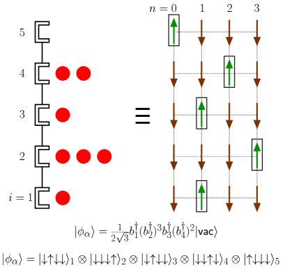
Figure 2.9: Mapping of the bosonic state $|{\phi_{\alpha}}\rangle$, of a chain with 5 sites and 7 bosons ($N_{P}=3$), into a four-spin-1/2 (or four-qubit) state. The convention is $|{\uparrow_{j}}\rangle\equiv|{0_{j}}\rangle$ and $|{\downarrow_{j}}\rangle\equiv|{1_{j}}\rangle$.

By definition (see Eqs. 2.53, 2.55, and 2.56) $\bar{b}^{\dagger}_{j}\ |{n}\rangle_{j}=\sqrt{n+1}\ |{n+1}\rangle_{j}$, and this operator in the conventional model maps to

$$\bar{b}^{\dagger}_{j}\rightarrow\tilde{b}^{\dagger}_{j}=\sum\limits_{n=0}^{N_{P}-1}\sqrt{n+1}\ \sigma_{-}^{n,j}\sigma_{+}^{n+1,j},$$ (2.59)

where a pair $(n,j)$ refers to the $n$th qubit in the chain of qubits representing the $j$th bosonic mode. The Pauli creation and annihilation operators $\sigma_{\pm}^{k}$ were previously defined in Sec. 2.1. The operator $\bar{b}^{\dagger}_{j}$ acts then on the $(N_{P}+1)$-qubit chain representing the $j$th bosonic mode as

$$\tilde{b}^{\dagger}_{j}|{1_{0}\cdots 1_{n-1}0_{n}1_{n+1}\cdots 1_{N_{P}}}\rangle_{j}=\sqrt{n+1}\ |{1_{0}\cdots 1_{n}0_{n+1}1_{n+2}\cdots 1_{N_{P}}}\rangle_{j},$$ (2.60)

so its matrix representation in this basis is analogous to the matrix representation of $\bar{b}^{\dagger}_{j}$ in the basis of bosonic states.

Similarly, the number operator is mapped as

$$\bar{n}_{j}\rightarrow\tilde{n}_{j}=\sum\limits_{n=0}^{N_{P}}n\ \frac{\sigma_{z}^{n,j}+1}{2},$$ (2.61)

so its action over the corresponding logical states is

$$\tilde{n}_{j}|{1_{0}\cdots 1_{n-1}0_{n}1_{n+1}\cdots 1_{N_{P}}}\rangle_{j}=n\ |{1_{0}\cdots 1_{n}0_{n+1}1_{n+2}\cdots 1_{N_{P}}}\rangle_{j}.$$ (2.62)

Since the commutator $[\tilde{b}^{\dagger}_{j},\sum_{n=0}^{N_{P}}\sigma_{z}^{n,j}]=0$ the operators $\tilde{b}^{\dagger}_{j}$ ($\tilde{b}_{j}$) always keep states within the same subspace.

The Hamiltonian of Eq. 2.52 in terms of Pauli operators is then

$$\tilde{H}=\sum\limits_{j,j^{\prime}=1}^{N}\alpha_{jj^{\prime}}\ \tilde{b}^{\dagger}_{j}\tilde{b}^{\;}_{j^{\prime}}+\beta_{jj^{\prime}}\ \tilde{n}_{j}\tilde{n}_{j^{\prime}},$$ (2.63)

where the operators $\tilde{b}^{\dagger}_{j}$ ($\tilde{b}^{\;}_{j}$) are given by Eqs. 2.59, and $\tilde{n}_{j}$ by Eq. 2.61. In this way, physical properties of the bosonic system such as the spectrum of $H$ can be obtained using a QC made of qubits. The same methods can be used when simulating any other type of boson-preserving quantum system.

Preparation of Initial Bosonic States

As in the fermionic case, the most general bosonic state of an $N$-mode lattice system with a maximum of $N_{P}$ bosons per site can be written as a linear combination of bosonic product states like

$$|{\phi_{\alpha}}\rangle={\sf K}(b^{\dagger}_{1})^{n_{1}}(b^{\dagger}_{2})^{n_{2}}\cdots(b^{\dagger}_{N})^{n_{N}}\ |{\sf vac}\rangle,$$ (2.64)

where ${\sf K}$ is a normalization factor, $n_{j}$ is the number of bosons at site $j$ ($\max(n_{j})=N_{P}$), and $|{\sf vac}\rangle$ is vacuum or no-boson state, that is, $b_{j}|{\sf vac}\rangle=0\ \forall j$.

Using the mapping described in Eq. 2.3.3, the vacuum state in the conventional model maps as

$$|{\sf vac}\rangle\rightarrow|{0_{0}1_{1}\cdots 1_{N_{P}}}\rangle_{1}\otimes\cdots\otimes|{0_{0}1_{1}\cdots 1_{N_{P}}}\rangle_{N},$$ (2.65)

and the product state of Eq. 2.64 maps as

$$|{\phi_{\alpha}}\rangle=|{1_{0}\cdots 0_{n_{1}}\cdots 1_{N_{P}}}\rangle_{1}\otimes\cdots\otimes|{1_{0}\cdots 0_{n_{N}}\cdots 1_{N_{P}}}\rangle_{N}$$ (2.66)

(see Fig. 2.9 for an example).

The preparation of the mapped bosonic state $|{\phi_{\alpha}}\rangle$ on a QC made of qubits is then performed by flipping the states of the corresponding qubits from a fully polarized state (i.e., the logical state with all qubits in $|{1}\rangle$), using for example the flip operations $\sigma^{n,j}_{x}$. Nevertheless, more general bosonic states like

$$|{\psi}\rangle=\sum\limits_{\alpha=1}^{L}g_{\alpha}\ |{\phi_{\alpha}}\rangle$$ (2.67)

can also be realized as in the fermionic case. Again, the idea is to add $L$ ancillas (extra qubits), perform controlled evolutions on their states, and finally perform measurements on the state of the ancillas. The state is successfully prepared with probability $1/L$ [OGK01].

Bosonic Evolutions

Again, the idea is to represent certain bosonic unitary evolution operator $\tilde{U}(t)=e^{-i\tilde{H}t}$, where $\tilde{H}$ is some boson-preserving Hermitian operator such as the Hamiltonian of the system to be simulated (Eq. 2.52), in terms of Pauli operators (Eq. 2.63). Usually, a first order Trotter approximation [Suz93] also needs to be performed to separate those terms in $H$ that do not commute.

In general, $H=K+V$ (Eq. 2.52), where $K$ is a kinetic term and $V$ a potential term. The kinetic term is a linear combination of terms like $b^{\dagger}_{k}b^{\;}_{l}+b^{\dagger}_{l}b^{\;}_{k}$. Therefore, a single-step evolution operator $e^{i(b^{\dagger}_{k}b^{\;}_{l}+b^{\dagger}_{l}b^{\;}_{k})\Delta t}$ is mapped onto Pauli operators as

$$\exp\left[i\vartheta\sum\limits_{n,n^{\prime}=0}^{N_{P}-1}\sqrt{(n+1)(n^{\prime}+1)}\ [(\sigma_{x}^{n,k}\sigma_{x}^{n+1,k}+\sigma_{y}^{n,k}\sigma_{y}^{n+1,k})(\sigma_{x}^{n^{\prime},l}\sigma_{x}^{n^{\prime}+1,l}+\right.$$

$$\left.\sigma_{y}^{n^{\prime},l}\sigma_{y}^{n^{\prime}+1,l})+(\sigma_{x}^{n,k}\sigma_{y}^{n+1,k}-\sigma_{y}^{n,k}\sigma_{x}^{n+1,k})(\sigma_{x}^{n^{\prime},l}\sigma_{y}^{n^{\prime}+1,l}-\sigma_{y}^{n^{\prime},l}\sigma_{x}^{n^{\prime}+1,l})]\right],$$ (2.68)

where $\vartheta=\Delta t/8$ and $N_{P}$ is the maximal number of bosons per site. The terms in the exponent of Eq. 2.68 commute with each other, so the decomposition into elementary gates can be done using the methods described in Sec. 2.1.2. As an example, consider a system of two sites with maximal one boson per site ($N_{P}=1$). Thus, $2(1+1)=4$ qubits are needed for the simulation, and Eq. 2.59 implies that $\tilde{b}^{\dagger}_{1}=\sigma_{-}^{0,1}\sigma_{+}^{1,1}$ and $\tilde{b}^{\dagger}_{2}=\sigma_{-}^{0,2}\sigma_{+}^{1,2}$. The mapped bosonic operator $e^{i(b^{\dagger}_{1}b^{\;}_{2}+b^{\dagger}_{2}b^{\;}_{1})\Delta t}$ in terms of Pauli operators is

$$\exp(i\vartheta\sigma_{x}^{0,1}\sigma_{x}^{1,1}\sigma_{x}^{0,2}\sigma_{x}^{1,2})\times\exp(i\vartheta\sigma_{x}^{0,1}\sigma_{x}^{1,1}\sigma_{y}^{0,2}\sigma_{y}^{1,2})\times\ \ \ \ \ \ \ \ \ \$$ (2.69)

$$\exp(i\vartheta\sigma_{y}^{0,1}\sigma_{y}^{1,1}\sigma_{x}^{0,2}\sigma_{x}^{1,2})\times\exp(i\vartheta\sigma_{y}^{0,1}\sigma_{y}^{1,1}\sigma_{y}^{0,2}\sigma_{y}^{1,2})\times\exp(i\vartheta\sigma_{y}^{0,1}\sigma_{x}^{1,1}\sigma_{y}^{0,2}\sigma_{x}^{1,2})\times$$

$$\exp(-i\vartheta\sigma_{y}^{0,1}\sigma_{x}^{1,1}\sigma_{x}^{0,2}\sigma_{y}^{1,2})\times\exp(-i\vartheta\sigma_{x}^{0,1}\sigma_{y}^{1,1}\sigma_{y}^{0,2}\sigma_{x}^{1,2})\times\exp(i\vartheta\sigma_{x}^{0,1}\sigma_{y}^{1,1}\sigma_{x}^{0,2}\sigma_{y}^{1,2}),$$

and the decomposition of each of the terms in Eq. 2.69 in terms of single and two-qubit elementary gates can be done, again, using the methods described in Sec. 2.1.2. An example of the decomposition of the term $\exp\left(\frac{it}{8}\sigma_{x}^{0,1}\sigma_{y}^{1,1}\sigma_{y}^{0,2}\sigma_{x}^{1,2}t\right)$, where the qubits were relabeled as $(n,j)\equiv n+2j-1$ (e.g., $(0,1)\rightarrow 1$) is shown in Fig. 2.10.

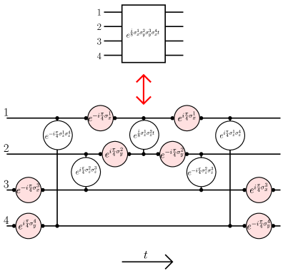
Figure 2.10: Decomposition of the unitary operator $\tilde{U}(t)=e^{\frac{it}{8}\sigma_{x}^{1}\sigma_{y}^{2}\sigma_{y}^{3}\sigma_{x}^{4}}$ into elementary gates as described in Sec. 2.1.2. The labeling convention is $(0,1)\equiv 1$, $(1,1)\equiv 2$, $(0,2)\equiv 3$, and $(1,2)\equiv 4$.

Contrary to the fermionic case, the number of elementary operations involved in the decomposition is not related to the distance between sites, $|k-l|$. Nevertheless, a physical bosonic operator $H$, such as the Hamiltonian of Eq. 2.52, involves a polynomially large number (with respect to $N$) of bosonic terms. Therefore, the corresponding evolution $\tilde{U}(t)=e^{-i\tilde{H}t}$ can be efficiently performed on a QC by applying a polynomially large number of elementary single and two-qubit gates. Again, when using approximate methods like the Trotter decomposition, the number of operations needed increases with the desired accuracy. However, such an approximation does not destroy the efficiency of the simulation.

2.4 Applications: The 2D fermionic Hubbard model

To clarify the methods described previously, in this section I present, as an example, the QS of the finite two-dimensional fermionic Hubbard model by using a CC that imitates a QC; that is, a quantum simulator. Since this is a classical simulation, the CC must keep track of an exponentially large number of quantum states, associated with the Hilbert space of the quantum system. Nevertheless, this simulation provides a good example for understanding the advantages and results that can be obtained when using a real QC.

The physical system to be simulated consists of a rectangular lattice (Fig. 2.11), with $N_{x}\times N_{y}$ sites, where spin-1/2 fermions hop from site to site under the interaction Hamiltonian

$$H=-\sum\limits_{(i,j);\sigma}[t_{x}c^{\dagger}_{(i,j);\sigma}c_{(i+1,j);\sigma}^{\;}+t_{y}c^{\dagger}_{(i,j);\sigma}c_{(i,j+1);\sigma}^{\;}+H.C.]+{\cal U}\sum\limits_{(i,j)}n_{(i,j);\uparrow}n_{(i,j);\downarrow}\ ,$$ (2.70)

where the operators $c^{\dagger}_{(i,j);\sigma}$ ($c_{(i,j);\sigma}$) create (annihilate) a fermion with spin component denoted by $\sigma$ ($=\uparrow$ or $\downarrow$), at the site located at $(x=i,y=j)$. $t_{x}$ and $t_{y}$ are the hopping terms in the $x$ and $y$ directions, respectively, and $n_{(i,j);\sigma}=c^{\dagger}_{(i,j);\sigma}c_{(i,j);\sigma}^{\;}$ is the corresponding number operator. ($H.C.$ denotes the Hermitian conjugate). Periodic boundary conditions (PBC) are assumed: $[(i,j);\sigma]\equiv=[(i+N_{x},j);\sigma]\equiv[(i,j+N_{y});\sigma]$.

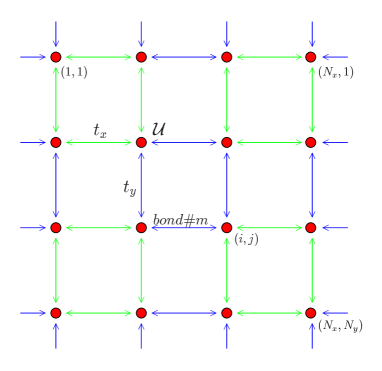
Figure 2.11: Two-dimensional lattice in the Hubbard model.

To use the QA for the obtention of the spectrum of $H$, described in Sec. 2.2.2, it is necessary first to map the fermionic operators onto Pauli operators using, for example, the Jordan-Wigner transformation (Sec. 2.3.1). Considering that these are spin-1/2 fermions, the QA needs $2(N_{x}\times N_{y})$ qubits to represent the system (qubits system), plus the ancilla qubit.

Assuming that one is mainly interested in obtaining the lowest energy of Eq. 2.70, the prepared initial state should be the ground state of Eq. 2.70. However, since no algebraic methods exist to exactly diagonalize Eq. 2.70 for large $N_{x}$ and $N_{y}$, such a state is not known, and therefore impossible to prepare. Nevertheless, the ground state of the associated mean-field Hamiltonian

$$H_{MF}=-\sum\limits_{(i,j);\sigma}[t_{x}c^{\dagger}_{(i,j);\sigma}c_{(i+1,j);\sigma}^{\;}+t_{y}c^{\dagger}_{(i,j);\sigma}c_{(i,j+1);\sigma}^{\;}+H.C.]+$$

$${\cal U}\sum\limits_{(i,j)}[\langle n_{(i,j);\uparrow}\rangle n_{(i,j);\downarrow}+n_{(i,j);\uparrow}\langle n_{(i,j);\downarrow}\rangle-\langle n_{(i,j);\uparrow}\rangle\langle n_{(i,j);\downarrow}\rangle]\ ,$$ (2.71)

is known to be a fermionic product state (Slater determinant) $|{\phi_{\beta}}\rangle$, and its corresponding state in the conventional model can be efficiently prepared by using the methods described in Sec. 2.3.1; that is, it can be prepared by applying a polynomially large (with respect to $N_{x}\times N_{y}$) set of elementary gates to the fully polarized state. For finite small lattices, $|{\phi_{\beta}}\rangle$ is a good approximation to the ground state of Eq. 2.70 and can be used to obtain the ground state energy.

The second step of the QA is to apply the unitary operator $\tilde{U}(t)=e^{i\tilde{H}\sigma_{z}^{\sf a}t/2}$ using single and two-qubit gates (see Fig. 2.8 for $\hat{Q}\equiv\tilde{H}$)), where, in this case, $\tilde{H}$ is the Hamiltonian of Eq. 2.70 in terms of Pauli operators, $t$ is a real (fixed) parameter, and $\sigma_{z}^{\sf a}$ is the Pauli operator associated with the ancilla qubit. Since $H$ is a linear combination of non-commuting terms (Eq. 2.70), the operator $\tilde{U}(t)=\prod_{j}\tilde{U}(\Delta t)$ can be approximated by using, for example, the first order Trotter decomposition [Suz93]. That is, $H=K_{\uparrow}+K_{\downarrow}+V$, where $K_{\sigma}$ denotes the kinetic energy associated with the fermions of spin $\sigma$ and $V$ denotes the potential energy. Then,

$$\tilde{U}(\Delta t)=e^{-i\tilde{H}\sigma_{z}^{\sf a}\Delta t/2}\sim e^{-i\tilde{K}_{\uparrow}\sigma_{z}^{\sf a}\Delta t/2}\times e^{-i\tilde{K}_{\downarrow}\sigma_{z}^{\sf a}\Delta t/2}\times e^{-i\tilde{V}\sigma_{z}^{\sf a}\Delta t/2},$$ (2.72)

where $\tilde{K}_{\sigma}$ and $\tilde{V}$ are the corresponding terms in Pauli operators. Also, the same approximation can be used to decompose each term $e^{-i\tilde{K}_{\sigma}\sigma_{z}^{\sf a}\Delta t/2}$. Such approximation leads to operators that can easily be decomposed in terms of elementary gates by using the methods described in Sec. 2.1.2.

The energy spectrum of the Hubbard model for a $4\times 2$ lattice is shown in Fig. 2.12. It has been obtained after running the classical simulation for many different values of $t$, and performing the Fourier transform on the data. The peaks show the eigenvalues and the results are compared to those of an exact diagonalization method.

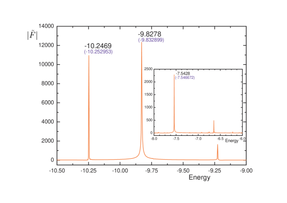
Figure 2.12: Energy spectrum of the Hubbard model obtained simulating the QA of Fig. 2.8 on a CC. The lattice has $4\times 2$ sites (which requires 16+1 qubits). Here, $t_{x}=t_{y}=1$, and ${\cal U}=4$. The time steps used in the Trotter approximation to prepare the initial state and apply the evolution are $\Delta t_{1}=\Delta t_{2}=0.05$, respectively. The numbers in brackets are the results obtained from the exact diagonalization using the Lanczos method.

The algorithm described allows one to easily obtain the energy spectra of a finite small lattice. Nevertheless, the spectra of a large lattice cannot be efficiently obtained using the same methods. The problem is that the ground state of the mean-field approximation differs more from the ground state of Eq. 2.70 as the system increases, and the QA needs to be performed an exponentially large number of times (with respect to $N_{x}\times N_{y}$) to obtain the desired property [SOG02].

2.5 Quantum Algorithms: Efficiency and Errors

A QA for a physical simulation is considered efficient if the total number of operations involved for the initial state preparation, the evolution, and the measurement process, scales at most polynomially with the system size and with $1/\epsilon$, where $\epsilon$ is the maximal tolerable error in the measurement of a relevant property.

While the decomposition of the operator $U(t)=e^{-iHt}$ can be done efficiently (e.g., when using the Trotter approximation) if $H$ is a physical operator, the preparation of a general initial state could be inefficient. Such inefficiency would arise, for example, if the state $|{\psi}\rangle$ defined in Eq. 2.37 or Eq. 2.67 is a linear combination of an exponentially large number of elementary product states. In this case, $L\sim x^{N}$, with $N$ the number of modes in the system and $x>1$, so an exponentially large number of trials need to be performed before successful preparation. However, if $L\leq\mbox{ poly}(N)$, it can be prepared efficiently. This construction generalizes to more general coherent states (see Chap. 4).

The three main reasons for the existence of errors $\epsilon$ in the outcome of the quantum computation are gate imperfections, the use of the Trotter approximation in the evolution operator, and the statistics in measuring the polarization of the ancilla qubit (Sec. 2.2.2). Gate imperfections are very common in quantum information because, contrary to classical information, quantum gates are usually dominated by a continuous parameter. This problem can be solved by using quantum error correction methods and fault tolerant quantum computation [Ste96, Kit97, NC00, Got97]. According to the accuracy threshold theorem, provided that the physical gates have sufficiently low error, it is possible to quantum compute accurately in an efficient way.

The type of error introduced by the discretization of the evolution operator $U(t)$ (e.g., by using the Trotter decomposition or other approximations) is very similar to the error obtained when performing a classical simulation, such as when using Monte Carlo methods. This error can be estimated by a detailed analysis of the discretization and can also be arbitrarily reduced in an efficient way.

Finally, when using the QAs described in Sec. 2.2.2, the step corresponding to the measurement process can also be performed efficiently because it only involves the measurement of a single (ancilla) qubit, regardless of the number of qubits needed for the simulation. Nevertheless, repeatedly many same-simulations need to be performed to get an accurate value of such measurement. This is an inherent property of the quantum mechanichs where a single measurement projects the quantum state (Sec. 2.1.1) and does not give sufficient information. If the relevant signal at the end of the quantum computation is small, like when obtaining the spectra of the two-dimensional Hubbard model on a large lattice (Sec. 2.4), it is necessary to run the algorithm a larger number of times and the efficiency can be destroyed.

In brief, a QC can only be more efficient than a CC when simulating quantum physical systems if the three main steps of the corresponding QA can be performed efficiently. For example, the evaluation of certain correlation functions over a quantum state that can be easily prepared, can be efficiently done with a QC. In general (i.e., for non-integrable Hamiltonians), there is no known way to evaluate such correlation efficiently with a CC [SOG02, SOK03].

2.6 Experimental Implementations of Quantum Algorithms

In this chapter, I have shown that if a large QC existed today, some simulations of quantum systems could be performed more efficiently on it than on a CC. Nevertheless, I did not discuss how the corresponding QAs could be experimentally implemented. Although numerous proposals for implementing quantum information processors (QIPs) are found in the literature [CZ95, CLK00, KLM01], only few of them have been successfully implemented to process more than one qubit. In particular, liquid-state NMR devices allow one to simulate several systems by manipulating, nowadays, up to ten qubits [RBC04].

The physical implementation of a large scale QC still remains one of the most important challenges for today’s physicists. The problem is a QC should be designed such that the interaction between its constituents and the environment is small enough to keep coherence of the quantum state. But if such interaction is too small, the manipulation and control processes using external sources becomes impracticable. For this reason, quantum decoherence has been one of the most important subjects of study during the last decade. In general, decoherence phenomena is hard to predict due to the infinite degrees of freedom associated with the environment. Nevertheless, a QC is reliable whenever the time required to perform a certain task is much smaller than the corresponding decoherence time.

In this section, I describe the experimental setting of a liquid-state NMR QIP and show how such devices can be used to execute the QAs described previously. Later on, I will show the experimental NMR simulation of a particular fermionic system, where some correlation functions and energy spectra have been obtained.

2.6.1 Liquid-State NMR Quantum Information Processor

Liquid-state NMR methods allow one to physically implement a slightly different version of the conventional model of quantum computation, with respect to the initial state preparation and the measurement process. In this set-up the quantum register is represented by the average state of the nuclear spin-1/2 of an ensemble of identical molecules. Each nuclear spin is a two-level physical system and can then be considered a possible qubit. Thus, the idea is to perform single and two-qubit elementary gates by external radio-frequency (rf) pulses that interact with the nuclear spin state. In the following, I present a basic analysis about how these processors can be used as possible QCs.

In a liquid NMR setting, the molecules are placed in a strong magnetic field $B(\hat{z})\simeq 10$ T, so that the spin of the $j$-th nucleus of a single molecule precesses at its Larmor frequency $\nu_{j}$ (Fig. 2.13). In the frame rotating with the $j$th spin, its qubit state can then be rotated by sending rf pulses in the XY plane at the resonant frequency $\nu_{r}\approx\nu_{j}$. If the duration of this pulse is $\delta t$, the corresponding evolution operator in the rotating frame is [LKC02]

$$U_{j}=e^{-iH_{j}\delta t}=e^{-i{\sf A}(\cos(\varphi)\sigma_{x}^{j}+\sin(\varphi)\sigma_{y}^{j})\delta t},$$ (2.73)

where ${\sf A}$ is the amplitude of the RF-pulse and $\varphi$ is its phase (i.e., orientation) in the XY plane ($\hbar=1$). Then, one can induce single spin rotations around any axis in that plane by adjusting $\delta t$ and $\varphi$.

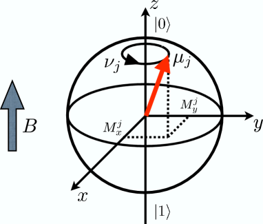
Figure 2.13: Bloch’s sphere representation of a single nuclear spin-1/2 state precessing around the quantization axis determined by the external magnetic field $B$. The precession frequency is given by $\nu_{j}=\mu_{j}B$, with $\mu_{j}$ the magnetic moment of the $j$th nucleus. Due to the chemical environment, each nucleus precesses at a different Larmor frequency $\nu_{j}$.

Single-qubit rotations around the $z$ axis can be implemented with no experimental imperfection or physical duration simply by changing the phase of the abstract rotating frame with which one is working. One has then to keep track of all these phase changes with respect to a reference phase associated with the spectrometer. Nevertheless, these phase tracking calculations are linear with respect to the number of pulses and spins, and can be efficiently done on a classical computer. Together with the rotations around any axis in the XY plane, the $z$ rotations can generate any single qubit rotation on the Bloch sphere.

Two-qubit gates, like the Ising gate $R_{z^{j}z^{k}}(\omega)$ (Sec. 2.1.1), can be performed by taking advantage of the spin-spin interactions (i.e., nuclei interaction) present in the molecule, and then achieve universal control. To first order in perturbation, this interaction, named the $J$-coupling, has the form

$$H_{j,k}=\frac{J_{jk}}{4}\sigma_{z}^{j}\sigma_{z}^{k},$$ (2.74)

where $j,k$ denote the corresponding pair of qubits and $J_{jk}$ is their coupling strength. Under typical NMR operating conditions, these interaction terms are small enough to be neglected when performing single-qubit rotations with rf pulses of short duration. Nevertheless, between two pulses they are driving the evolution of the system. By cleverly designing a pulse sequence, i.e., a succession of pulses and free evolution periods, one can easily apply two-qubit gates on the state of the system. Indeed, the so-called refocusing techniques’ principle consists of performing an arbitrary Ising gate by flipping one of the coupled spins ($\pi$-pulse), as shown in Fig 2.14. The interaction evolutions before and after the refocusing pulse compensate, leading to the effective evolution

$$U^{\sf eff}_{j,k}=e^{i\frac{\pi}{2}\sigma_{x}^{j}}e^{-i\frac{J_{jk}}{4}\sigma_{z}^{j}\sigma_{z}^{k}\delta t_{2}}e^{-i\sigma_{x}^{j}\pi/2}e^{-i\frac{J_{jk}}{4}\sigma_{z}^{j}\sigma_{z}^{k}\delta t_{1}}=e^{-i\frac{\bar{\alpha}}{4}\sigma_{z}^{j}\sigma_{z}^{k}},$$ (2.75)

where the effective coupling strength $\bar{\alpha}=J_{jk}(\delta t_{1}-\delta t_{2})$ is being determined by the difference between the durations $\delta t_{1}$ and $\delta t_{2}$.

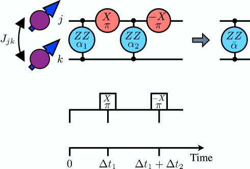
Figure 2.14: Circuit representation for the refocusing scheme to control $J$ couplings. The Ising-like coupling $J_{jk}$ between spins can be controlled by performing flips on one of the spins at times $t_{1}=\Delta t_{1}$ and $t_{2}=t_{1}+\Delta t_{2}$, respectively. The effective coupling is $\bar{\alpha}=\alpha_{1}-\alpha_{2}=J_{jk}(\Delta t_{1}-\Delta t_{2})$, and vanishes when $\Delta t_{1}=\Delta t_{2}$.

Although the physics on a single molecule has been analyzed, liquid-state NMR uses an ensemble of about $10^{23}$ molecules in a solution maintained at room temperature ($\simeq 300K$). For typical values of the magnetic field, this thermal state is extremely mixed. Clearly, this is not the usual state in which one initializes a quantum computation since qubits are nearly randomly mixed. Nevertheless, known NMR methods [LKC02] can be used to prepare the so-called pseudo-pure state ($\rho_{\sf pp}$)

$$\rho_{{\sf pp}}=\frac{(1-\bar{\epsilon})}{2^{N}}{\mathchoice{\rm 1\mskip-4.0mul}{\rm 1\mskip-4.0mul}{\rm 1\mskip-4.5mul}{\rm 1\mskip-5.0mul}}+\bar{\epsilon}\rho_{{\sf pure}},$$ (2.76)

where ${\mathchoice{\rm 1\mskip-4.0mul}{\rm 1\mskip-4.0mul}{\rm 1\mskip-4.5mul}{\rm 1\mskip-5.0mul}}$ is the identity operator, $\rho_{{\sf pure}}$ is a density operator that describes a pure state, and $\bar{\epsilon}$ is a small real constant (i.e., $\bar{\epsilon}$ decays exponentially with the number of atoms in the solution due to the Boltzmann’s distribution).

Under the action of any unitary evolution $U$, this state evolves as

$$\rho_{\sf pp}^{\sf final}=U\rho_{\sf pp}U^{\dagger}=\frac{(1-\bar{\epsilon})}{2^{N}}{\mathchoice{\rm 1\mskip-4.0mul}{\rm 1\mskip-4.0mul}{\rm 1\mskip-4.5mul}{\rm 1\mskip-5.0mul}}+U\bar{\epsilon}\rho_{{\sf pure}}U^{\dagger}.$$ (2.77)

The first term in Eq. 2.77 did not change because the identity operator is invariant under any unitary transformation. Therefore, performing quantum computation on the ensemble is equivalent to performing quantum computation over the initial state represented only by $\rho_{{\sf pure}}$.

At the end of the computation, the orthogonal components of the sample polarization in the XY plane, $M_{x}={\sf Tr}(\rho_{\sf pp}^{\sf final}\sum_{i=1}^{N}\sigma_{x}^{i})$, and $M_{y}={\sf Tr}(\rho_{\sf pp}^{\sf final}\sum_{i=1}^{N}\sigma_{y}^{i})$ are measured (Eq. 2.15). Note that the invariant component of $\rho_{\sf pp}^{\sf final}$ does not contribute to the signal since ${\sf Tr}({\mathchoice{\rm 1\mskip-4.0mul}{\rm 1\mskip-4.0mul}{\rm 1\mskip-4.5mul}{\rm 1\mskip-5.0mul}}\sigma_{x,y}^{j})=0$. Because the polarization of each single spin, $M_{x}^{j}={\sf Tr}(\rho_{\sf pp}^{\sf final}\sigma_{x}^{j})$ and $M_{y}^{j}={\sf Tr}(\rho_{\sf pp}^{\sf final}\sigma_{y}^{j})$, precesses at its own Larmor frequency $\nu_{j}$, a Fourier transformation of the temporal recording (called FID, for Free Induction Decay) of the total magnetization needs to be performed. By doing so, one obtains the expectation value of the polarization of each spin (averaged over all molecules in the sample).

Summarizing, a liquid-state NMR setting allows one to initialize a register of qubits in a pseudo-pure state, apply any unitary transformation to this state by sending controlled rf pulses or by leaving free interaction periods, and measure the expectation value of some quantum observables (i.e., the spin polarization). Hence, these systems can be used as QIPs.

2.7 Applications: The Fano-Anderson Model

I now present the experimental QS of the fermionic one-dimensional (1D) Fano-Anderson model using a liquid-state NMR [NSO05], by manipulating the state of the spin nuclei as described in Sec. 2.6.1. Such simulation shows then how reliable these experimental methods are and how well the elementary gates (Sec. 2.1.1) can be implemented using NMR techniques.

The 1D fermionic Fano-Anderson model consists of an $n$-sites ring with an impurity in the center (Fig. 2.15), where spinless fermions can hop between nearest-neighbors sites with hopping matrix element (overlap integral) $\tau$, or between a site and the impurity with matrix element $V/\sqrt{n}$. Taking the single-particle energy of a fermion in the impurity to be $\epsilon$, and considering the translational invariance of the system, the Fano-Anderson Hamiltonian can be written in the wave vector representation as [OGK01]

$$H=\sum_{l=0}^{n-1}\varepsilon_{k_{l}}c^{\dagger}_{k_{l}}c_{k_{l}}^{\;}+\epsilon b^{\dagger}b+V(c^{\dagger}_{k_{0}}b+b^{\dagger}c_{k_{0}}^{\;}),$$ (2.78)

where the fermionic operators $c^{\dagger}_{k_{l}}$ and $b^{\dagger}$ ($c_{k_{l}}^{\;}$ and $b$) create (destroy) a spinless fermion in the conduction mode $k_{l}$ and in the impurity, respectively. Here, the wave vectors (modes) are $k_{l}=\frac{2\pi l}{n}$ ($l=[0,..,n-1]$) and the energies per mode are $\varepsilon_{k_{l}}=-2\tau\cos k_{l}$.

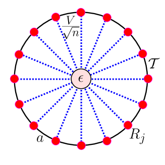
Figure 2.15: Fermionic Fano-Anderson model. Fermions can hop between nearest neighbor sites (exterior circles) and between a site and the impurity (centered circle), with hopping matrix elements $\tau$ and $V/{\sqrt{n}}$, respectively. The energy of localization in the impurity is $\epsilon$.

In this form, the Hamiltonian in Eq. 2.78 is almost diagonal and can be exactly solved: There are no interactions between fermions in different modes $k_{l}$, except for the mode $k_{0}$, which interacts with the impurity. Therefore, the relevant physics comes from this latter interaction, and its spectrum can be exactly obtained by diagonalizing a $2\times 2$ Hermitian matrix, regardless of $n$ and the number of fermions in the ring, $N_{e}$. Nevertheless, its simulation in a liquid-state NMR QIP is the first step in QSs of quantum many-body problems and constitutes a proof of the principles described throughout this thesis.

In order to successfully simulate this system in a liquid-state NMR QIP, the fermionic operators need to be mapped onto the Pauli operators (Sec. 2.3.1). This is done by using the following Jordan-Wigner transformation

$$\matrix{b=\sigma_{-}^{1}&b^{\dagger}=\sigma_{+}^{1}\cr c^{\;}_{k_{0}}=-\sigma_{z}^{1}\sigma_{-}^{2}&c^{\dagger}_{k_{0}}=-\sigma_{z}^{1}\sigma_{+}^{2}\cr\vdots&\vdots\cr c^{\;}_{k_{n-1}}=\left(\prod_{j=1}^{n}-\sigma_{z}^{j}\right)\sigma_{-}^{n+1}&\qquad c^{\dagger}_{k_{n-1}}=\left(\prod_{j=1}^{n}-\sigma_{z}^{j}\right)\sigma_{+}^{n+1}.}$$ (2.79)

In this language, a logical state $|{0_{j}}\rangle$ (with $|{0}\rangle\equiv|{\uparrow}\rangle$ in the usual spin-1/2 notation) corresponds to having a spinless fermion in either the impurity, if $j=1$, or in the mode $k_{j-2}$, otherwise (Fig. 2.16). (Again, the fermionic vacuum state $|{{\sf vac}}\rangle$ maps onto $|{{\sf\widehat{vac}}}\rangle=|{1_{1}1_{2}\cdots 1_{n+1}}\rangle$.)

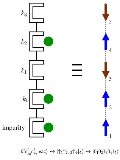
Figure 2.16: Mapping of the fermionic product state $b^{\dagger}c^{\dagger}_{k_{0}}c^{\dagger}_{k_{2}}|{\sf vac}\rangle$ into a five-qubit state, using the Jordan-Wigner transformation. The convention is $|{\uparrow_{j}}\rangle\equiv|{0_{j}}\rangle$ (filled) and $|{\downarrow_{j}}\rangle\equiv|{1_{j}}\rangle$ (empty).

The algorithms described in Sec. 2.2.2 can be used, for example, to evaluate the probability amplitude of having a fermion in mode $k_{0}$ at time $t$, if initially ($t=0$) the quantum state is the Fermi sea state with $N_{e}$ fermions; that is, $|{\sf FS}\rangle=\prod\limits_{l=0}^{N_{e}-1}c^{\dagger}_{k_{l}}|{{\sf vac}}\rangle$. This probability is given by the modulus square of the following dynamical correlation function:

$$G(t)=\langle{\sf FS}|b(t)b^{\dagger}(0)|{\sf FS}\rangle\ ,$$ (2.80)

where $b(t)=T^{\dagger}b(0)T$, $T=e^{-iHt}$ is the time evolution operator, and $b^{\dagger}(0)=b^{\dagger}$. Basically, $G(t)$ is the overlap between the quantum state $b^{\dagger}(0)|{\sf FS}\rangle$, which does not evolve, and the state $b^{\dagger}(t)|{\sf FS}\rangle$, which does not vanish unless the evolved state $T|{\sf FS}\rangle$ already contains a fermion in the impurity site ($(b^{\dagger}(t))^{2}=(b^{\dagger}(0))^{2}=0$), i.e., contains the fermion which initially was in the $k_{0}$ mode. In terms of Pauli operators (see Eq. 2.79), this correlation function reduces to a two-qubit problem [OGK01]:

$$G(t)=\langle{\phi}|\bar{T}^{\dagger}\sigma_{-}^{1}\bar{T}\sigma_{+}^{1}|{\phi}\rangle\ ,$$ (2.81)

where $\bar{T}=e^{-i\bar{H}t}$ is an evolution operator arising from the interaction terms in Eq. 2.78, with

$$\bar{H}=\frac{\epsilon}{2}\sigma_{z}^{1}+\frac{\varepsilon_{k_{0}}}{2}\sigma_{z}^{2}+\frac{V}{2}(\sigma_{x}^{1}\sigma_{x}^{2}+\sigma_{y}^{1}\sigma_{y}^{2})\ ,$$ (2.82)

and $|{\phi}\rangle=|{1_{1}0_{2}}\rangle$ in the logical basis (i.e., the initial state with one fermion in the $k_{0}$ mode).

In order to use the quantum circuit depicted in Fig. 2.7, all operators in Eq. 2.81 must be unitary. Because of the symmetries of $\bar{H}$, such as the global $\pi/2$-$z$ rotation that maps $(\sigma_{x}^{j},\sigma_{y}^{j})\rightarrow(\sigma_{y}^{j},-\sigma_{x}^{j})$, leaving the state $|{\phi}\rangle$ invariant (up to a phase factor), then $\langle\phi|\bar{T}^{\dagger}\sigma_{x}^{1}\bar{T}\sigma_{y}^{1}|{\phi}\rangle=\langle\phi|\bar{T}^{\dagger}\sigma_{y}^{1}\bar{T}\sigma_{x}^{1}|{\phi}\rangle=0$ and $\langle\phi|\bar{T}^{\dagger}\sigma_{x}^{1}\bar{T}\sigma_{x}^{1}|{\phi}\rangle=\langle\phi|\bar{T}^{\dagger}\sigma_{y}^{1}\bar{T}\sigma_{y}^{1}|{\phi}\rangle$. Therefore, Eq. 2.81 can be written in terms of unitary operators as

$$G(t)=\langle{\phi}|e^{i\bar{H}t}\sigma_{x}^{1}e^{-i\bar{H}t}\sigma_{x}^{1}|{\phi}\rangle.$$ (2.83)

Figure 2.17 shows the quantum circuit used to obtain $G(t)$. It is derived from Fig. 2.7 by making the following identifications: $T\rightarrow e^{-i\bar{H}t}$, $A_{i}\rightarrow\sigma_{x}^{1}$, and $B_{j}\rightarrow\sigma_{x}^{1}$. The corresponding controlled operations C-A and C-B transform into the well-known controlled-not (CNOT) gates (Sec. 2.1.3). All the unitary operations appearing in Fig. 2.17 were decomposed into elementary NMR gates (single qubit rotations and Ising interactions). In particular, the decomposition of $e^{-i\bar{H}t}$ can be found in Ref. [OGK01], obtaining

$$e^{-i\bar{H}t}=Ue^{-i\lambda_{1}\sigma_{z}^{1}t}e^{-i\lambda_{2}\sigma_{z}^{2}t}U^{\dagger}\ ,$$ (2.84)

where $\lambda_{1(2)}=\frac{1}{2}(E\mp\sqrt{\Delta^{2}+V^{2}})$, with $E=\frac{\epsilon+\varepsilon_{k_{0}}}{2}$, and $\Delta=\frac{\epsilon-\varepsilon_{k_{0}}}{2}$. The unitary operator $U$ is decomposed as (Fig. 2.17)

$$U=e^{i\frac{\pi}{4}\sigma^{2}_{x}}e^{-i\frac{\pi}{4}\sigma^{1}_{y}}e^{-i\frac{\theta}{2}\sigma^{1}_{z}\sigma^{2}_{z}}e^{i\frac{\pi}{4}\sigma^{1}_{y}}e^{i\frac{\pi}{4}\sigma^{1}_{x}}e^{-i\frac{\pi}{4}\sigma^{2}_{x}}e^{-i\frac{\pi}{4}\sigma^{2}_{y}}e^{i\frac{\theta}{2}\sigma^{1}_{z}\sigma^{2}_{z}}e^{-i\frac{\pi}{4}\sigma^{1}_{x}}e^{i\frac{\pi}{4}\sigma^{2}_{y}},$$ (2.85)

with the parameter $\theta$ satisfying $\cos\theta=1/\sqrt{1+\delta^{2}}$, and $\delta=(\Delta+\sqrt{\Delta^{2}+V^{2}})/V$.

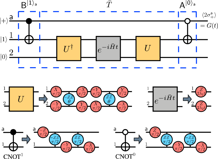
Figure 2.17: Quantum circuit for the evaluation of $G(t)$ (Eq. 2.80) in terms of elementary gates directly able to be implemented with liquid-state NMR methods. The controlled operations ${\sf B}^{|{1}\rangle_{\sf a}}$ and ${\sf A}^{|{0}\rangle_{\sf a}}$ correspond to the operations C-B and C-A of Sec. 2.2.2, respectively.

The CNOT gates C-A and C-B can also be decomposed into elementary gates, as explained in Sec. 2.1.2. Therefore, $G(t)$ can be obtained using an NMR QIP by applying the appropriate rf pulses (Sec. 2.6.1). Remarkably, only three qubits are required for the simulation (Fig. 2.17): The ancilla qubit ${\sf a}$, one qubit representing the impurity site (qubit-1), and one qubit representing the $k_{0}$ mode (qubit-2).

Similarly, the algorithm depicted in Fig. 2.8 can be used if interested in obtaining the spectrum of the Hamiltonian $H$ of Eq. 2.78, replacing $\hat{Q}\rightarrow H$. In particular, when $n=1$ (one site plus the impurity), Eq. 2.78 in terms of Pauli operators reduces to $\tilde{H}=\frac{\epsilon+\varepsilon_{k_{0}}}{2}+\bar{H}$, with $\bar{H}$ defined in Eq. 2.82. In this case, the two eigenvalues $\lambda_{i}$ ($i=1,2$) of the one-particle subspace can be extracted from the correlation function

$$S(t)=\langle{\phi}|e^{-i\tilde{H}t}|{\phi}\rangle=e^{-i(\epsilon+\varepsilon_{k_{0}})t}\langle{\phi}|e^{-i\bar{H}t}|{\phi}\rangle,$$ (2.86)

which can be obtained by measuring the polarization of the ancilla qubit after the quantum circuit shown in Fig. 2.8 has been applied. Since $|{\phi}\rangle=|{1_{1}0_{2}}\rangle$ is not an eigenstate of $H$, it has a non-zero overlap with the two one-particle eigenstates, called $|{{\sf 1P}_{i}}\rangle$ (see Appendix B).

Again, the operator $e^{i\tilde{H}\sigma_{z}^{\sf a}t/2}$ (Fig. 2.8) needs to be decomposed into elementary gates for its implementation in an NMR QIP. Noticing that $[\sigma_{z}^{\sf a},\tilde{H}]=[\sigma_{z}^{\sf a},U]=0$, then

$$e^{i\tilde{H}\sigma_{z}^{\sf a}t/2}=Ue^{i\lambda_{1}\sigma_{z}^{1}\sigma_{z}^{\sf a}t/2}e^{i\lambda_{2}\sigma_{z}^{2}\sigma_{z}^{\sf a}t/2}U^{\dagger}e^{i(\epsilon+\varepsilon_{k_{0}})\sigma_{z}^{\sf a}t/2},$$ (2.87)

where the unitary operator $U$ is decomposed as in Eq. 2.85. Figure 2.18 shows the corresponding circuit in terms of elementary gates. Again, qubits 1 and 2 represent the impurity site and the $k_{0}$ mode, respectively. ${\sf a}$ denotes the ancilla qubit. Since the idea is to perform a DFT on the results obtained from the measurement (see Appendix B), this circuit needs to be applied for several values of the parameter $t$ (Sec. 2.1.3).

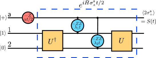
Figure 2.18: Quantum circuit for the evaluation of $S(t)$ [Eq. 2.86]. The parameters $\lambda_{1}$ and $\lambda_{2}$ are defined in Sec. 2.7, and $\alpha=(\epsilon+\varepsilon_{k_{0}})/2$. The decomposition of the operator $U$ in NMR gates is shown in Fig. 2.17.

2.7.1 Experimental Protocol and Results

The NMR setting used for the evaluation of $G(t)$ and $S(t)$ is based on an ensemble solution of trans-crotonic acid and methanol dissolved in acetone (Fig. 2.19). This molecule can be used as a seven-qubit register, where methanol is used to perform rf-power selection and accurately calibrate the rf pulses. In this way, the decoherence time ($T_{2}^{*}$) is in the range from several hundreds of milliseconds to more than a second, allowing one to perform around 1000 single-qubit gates and around 100 two-qubit (Ising) gates.

Figure 2.19: The transcrotonic acid molecule is a seven-qubit register. The methyl group is used as a single qubit [KLM00]. The table shows the values of the chemical shifts (main diagonal) and the $J$ couplings (off-diagonal) between every pair of nuclei or qubits, in hertz.

The relevant nuclei of the molecule are denoted as $\mbox{C}_{1}$, $\mbox{C}_{2}$, $\mbox{C}_{3}$, and $\mbox{C}_{4}$, corresponding to the Carbon atoms, $\mbox{H}_{1}$ and $\mbox{H}_{2}$ corresponding to the Hydrogen atoms, and M corresponding to the methyl group. Although this is a seven-qubit register, the simulation of the Fano-Anderson model requires only three qubits. Considering different practical issues, such as the nuclei-nuclei interaction, the selection has been made as follows: The spin nucleus $\mbox{C}_{1}$ represents qubit-1, the spin nucleus M represents qubit-2, and the spin nucleus $\mbox{C}_{2}$ represents the ancilla qubit ${\sf a}$.

The idea is then to apply the desired elementary gates by sending appropriate rf pulses. Nevertheless, designing a pulse sequence to implement exactly the desired unitary transformation would require very long refocusing schemes to cancel out all the unwanted naturally occurring $J$ couplings (free evolutions). Then, the overall duration of the pulse sequence increases and decoherence effects could destroy the signal. Therefore, a pulse sequence compiler is used to approximate the evolution and numerically optimize the delays between pulses to minimize the error introduced by such approximation.

The approximate evolution is then applied to the corresponding initial state $\rho_{\sf init}=\frac{1}{2}\left[({\mathchoice{\rm 1\mskip-4.0mul}{\rm 1\mskip-4.0mul}{\rm 1\mskip-4.5mul}{\rm 1\mskip-5.0mul}}^{\mbox{C}_{2}}+\sigma_{x}^{\mbox{C}_{2}})\mbox{\bf 1}^{\mbox{C}_{1}}\mbox{\bf 0}^{\mbox{M}}\right]$, which is the density operator corresponding to the pure state $|{+}\rangle_{\sf a}|{1_{1}0_{2}}\rangle$. Since the identity part ${\mathchoice{\rm 1\mskip-4.0mul}{\rm 1\mskip-4.0mul}{\rm 1\mskip-4.5mul}{\rm 1\mskip-5.0mul}}^{\mbox{C}_{2}}$ is not an observable, the pseudo-pure state $\rho^{\prime}_{\sf init}=\sigma_{x}^{\mbox{C}_{2}}\mbox{\bf 1}^{\mbox{C}_{1}}\mbox{\bf 0}^{\mbox{M}}$, with $\mbox{\bf 1}\equiv|{1}\rangle\langle{1}|$ and $\mbox{\bf 0}\equiv|{0}\rangle\langle{0}|$, can be used equivalently. Then $\rho^{\prime}_{\sf init}$, which is a deviation of the completely mixed state due to the high temperature of the ensemble (Sec. 2.6.1), can easily be prepared using already developed NMR techniques [LKC02].

As mentioned in Sec. 2.2.2, the desired result of the QA is encoded in the polarization $\langle 2\sigma_{+}^{\mbox{C}_{2}}\rangle$ of the nucleus $\mbox{C}_{2}$ (i.e., ancilla qubit). This component precesses at the $\mbox{C}_{2}$-Larmor frequency $\nu_{\mbox{C}_{2}}$. To measure it, a Fourier transformation on the measured free induction decay FID (i.e., the decay in the polarization due to the contribution of different Larmor frequencies) must be performed, integrating only the peak located at $\nu_{\mbox{C}_{2}}$. Nevertheless, the absolute value of this signal is irrelevant since it depends on many experimental parameters such as the solution concentration, the probe sensitivity, and the gain of the amplifier. The relevant quantity is its intensity relative to a reference signal given by the observation of the initial state $\rho_{\sf init}$. To get a good signal-to-noise ratio, each experiment (or scan) was done several times and the corresponding experimental data were added. Moreover, to average over small magnetic fluctuations occurring within the duration of the whole experiment the scans of the reference experiment (i.e., the measurement of the reference signal) are interlaced with scans of the actual complete pulse sequence. To increase the spatial homogeneity of the field over the sample, several automated shimming periods, consisting of fine tuning small additional coils located around the sample, have been inserted.

In Fig. 2.20, I show the experimental results obtained for the evaluation of $G(t)$ for $\varepsilon_{k_{0}}=-2\mbox{, }\epsilon=-8,\ V=4,$ and $\varepsilon_{k_{0}}=-2\mbox{, }\epsilon=0\mbox{, }V=4$, and for different values of $t$. The duration of the optimized pulse sequences from the beginning of the initialization step to the beginning of the data acquisition, was 97 ms. For comparison, the analytical form of $G(t)$, as well as the simulated data points (i.e., data points obtained by simulating the quantum algorithm on a conventional computer) are also shown in the figure.

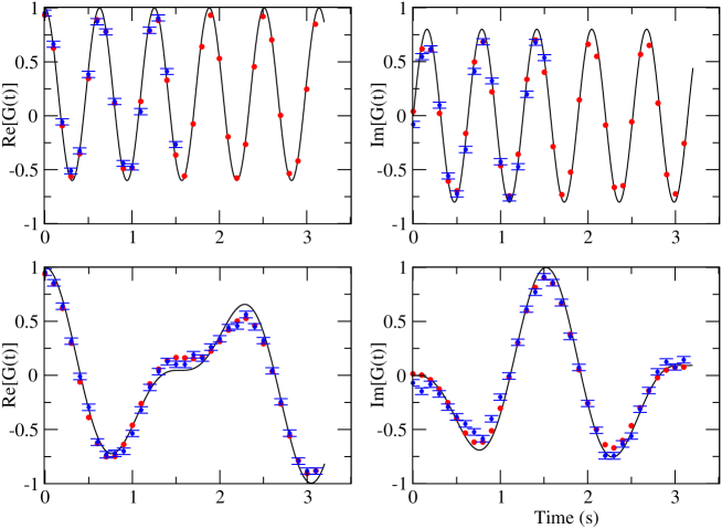
Figure 2.20: Real and imaginary parts of the correlation function $G(t)$ of Eq. 2.80. The top panels show the results when the parameters in Eq. 2.78 are $\varepsilon_{k_{0}}=-2,\epsilon=-8,V=4$. The corresponding parameters $\lambda_{1},\lambda_{2},\theta$ can be determined using Eqs. 2.84 and 2.85. The bottom panels show the results for $\varepsilon_{k_{0}}=-2,\epsilon=0,V=4$. The (black) solid line is the analytic solution, the red circles are obtained by the numerical simulation (including the refocusing pulses), and the blue circles with the error bars are experimental data.

In Fig. 2.21, I present the experimental results obtained for the evaluation of $S(t)$, to obtain the corresponding eigenvalues for the Hamiltonian, with $\varepsilon_{k_{0}}=-2,\ \epsilon=-8$, and $V=0.5$. The pulse sequence applied is the one corresponding to the quantum circuit shown in Fig. 2.18 with the corresponding refocusing pulses. In Fig. 2.21, I also show the analytical and simulated data points. The DFT of the experimental data is shown in Fig. 2.22, revealing the expected peaks at the frequency corresponding to the two one-particle eigenvalues of Eq. 2.78, for the above parameters.

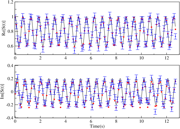
Figure 2.21: Real and imaginary parts of $S(t)$, for $\varepsilon_{k_{0}}=-2,\ \epsilon=-8$, and $V=0.5$ in Eq. 2.78. The (black) solid line corresponds to the analytic solution. The red circles correspond to the numerical simulation (using refocusing pulses) and the blue circles with the error bars are experimental data. $S(t)$ has been measured using the network of Fig. 2.18 with $\alpha=(\epsilon+\varepsilon_{k_{0}})/2$.

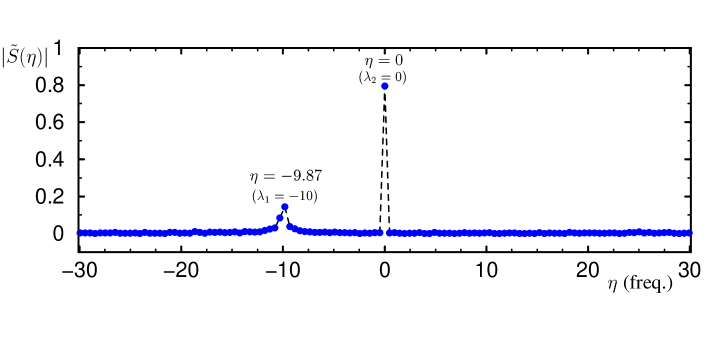
Figure 2.22: Discrete Fourier transform of the real part of the experimental data of Fig. 2.21. The position of the two peaks corresponds to the two eigenvalues of the Hamiltonian of Eq. 2.78 for $\varepsilon_{k_{0}}=-2,\epsilon=-8$, and $V=0.5$. Numbers in parentheses denote the exact solution. The size of the dots representing experimental points is the error bar (see Appendix B). An upper bound to the error in the frequency domain is $\approx 0.5$, which was determined by the resolution of the spectrum due to the time sampling of the simulation.

The close agreement between the experimental results and the corresponding simulations, using the refocusing pulses, suggests that the main contribution to errors comes from the incomplete refocusing scheme used in the optimization procedure. Therefore, increasing the number of refocusing pulses might have led to more accurate results even if they would have increased the overall duration of the pulse sequence.

2.8 Summary

Throughout this chapter, I have addressed several broad issues associated with the simulation of physical phenomena with QCs. In particular, I presented efficient ways to map the algebras of operators associated to the physical system to be simulated onto the algebra of Pauli operators. These mappings are sufficient to establish the equivalence of the different physical models to a universal model of quantum computation: The conventional model.

I also explored various issues associated with simulations (Sec. 2.3), remarking that every step in a QA must be performed efficiently to have an efficient simulation. Although a QC can simulate some quantum physical systems more efficiently than its classical analogue, I showed that many challenges still remain to prove this statement in a general way (Sec. 2.5). As an example, I presented the QS of the two-dimensional fermionic Hubbard model, where there is no known way to obtain its ground state energy efficiently using a QC.

Finally, I described the experimental implementation of a QA using a liquid-state NMR QIP (Sec. 2.7). This experiment allows one to understand the advantages and disadvantages of simulating physical systems with today’s QCs, and, in particular, to understand the power of quantum computation.

Chapter 3 Quantum Entanglement as an Observer-Dependent Concept

“…Maximal knowledge of a total (quantum) system does not necessarily include total knowledge of all its parts, not even when these are fully separated from each other and at the moment are not influencing each other at all.”

E. Schrödinger (1935).

Quantum Entanglement (QE) is referred to the existence of certain correlations in a quantum system that have no classical interpretation. This concept was first introduced by E. Schrödinger [Sch35] as the essence of quantum mechanics, and is responsible for many counterintuitive physical processes like the violation of the local realism. Naturally, it has been the main focus of philosophical discussions since the early days of quantum mechanics, and it is now known that entanglement is the defining resource that allows one to perform certain protocols like quantum cryptography, quantum teleportation, and even more efficient computation. For this reason, QE has been one of the most important subjects of study in QIT during recent years. Nevertheless, its analysis requires a good understanding of the conceptual foundations of the quantum theory. For this purpose, a historical introduction to the subject is given in the following sections.

The EPR Paradox

In 1935, Einstein, Podolsky and Rosen designed an experiment, the so called EPR paradox [EPR35], to prove that quantum mechanics was an incomplete description of physical reality. Neither they nor others agreed that the (probabilistic) outcome of a measurement performed on a quantum system was not uniquely determined by its quantum state $|{\psi}\rangle$. They believed, instead, that the result of a measurement was a property associated with the quantum system right before the measurement was performed.

To prove this statement, they considered a system composed of two quantum particles where, although the position and momentum of each particle were not well defined (uncertainty), the sum of their positions and the difference of their momenta were. For pedagogical purposes, I consider here a simpler version of this experiment by means of the conventional model [Boh51] where the qualitative results are equivalent to those of the EPR paradox. This simplified model consists of two qubits initially prepared in some state (Fig. 3.1)

$$|{\sf Bell}\rangle=\frac{1}{\sqrt{2}}\left[|{0_{\cal A}1_{\cal B}}\rangle-|{1_{\cal A}0_{\cal B}}\rangle\right].$$ (3.1)

[Such a state represents, for example, the singlet state (total spin 0) of two-spin 1/2.] Assuming that a measurement (in the logical basis) is performed on qubit $\cal A$, quantum mechanics says that the outcome of such measurement projects the state $|{\sf Bell}\rangle$ onto the state $|{0_{\cal A}1_{\cal B}}\rangle$ with probability 1/2, and onto the state $|{1_{\cal A}0_{\cal B}}\rangle$ with the same probability (Sec. 2.1.1). Thus, a measurement on qubit $\cal A$ projects also the state of qubit ${\cal B}$, such that the outcome of a later measurement performed on it can be predicted with certainty.

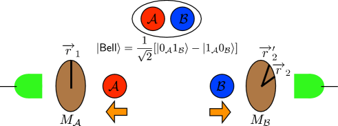
Figure 3.1: Bohm’s representation of J. Bell’s experiment. Two qubits in a pure quantum state are separated and their polarizations are locally measured along three different directions. The measurement outcomes violate the Bell inequality of Eq. 3.8. Here $M$ denotes the polarizers.

What worried Einstein and others is the fact that, in principle, both particles (qubits) could be very far apart in physical space. Therefore, a person located close to qubit $\cal A$ could gain information about the state of qubit ${\cal B}$ almost immediately, violating the principle of locality; that is, some information could be propagated at infinitely large speed. If such were the case, the existence of these quantum correlations would be against the relativity theory, and the understanding of the physical world would be completely different. Nevertheless, a deeper analysis shows that such violation does not exist and that quantum mechanics is right. Below, I present the experiments suggested by Bell to show that quantum correlations exist in nature and cannot be explained by means of classical theory.

Bell’s Inequalities

The idea of existence of hidden variables which determine the outcome of a measurement in a quantum system was proved to be incompatible with quantum mechanics by J. Bell [Bel64] in 1964. Basically, he proposed a similar experiment to the one described above but such that the measurements could be performed in any direction, that is, in a possible basis different to the logical one. For example, when working with photons, such measurements could be performed by using polarizers rotated by different angles.

Assuming that qubit ${\cal A}$ is measured in some basis denoted by the vector $\overrightarrow{r}_{1}$ and qubit ${\cal B}$ is measured in the basis denoted by $\overrightarrow{r}_{2}$, such measurements project the state of either qubit in the corresponding direction with eigenvalues $\pm 1$ (Sec. 2.1.1). In other words, the state after the measurement of the $j$th qubit can be represented as a vector pointing in the direction $\overrightarrow{r}_{j}$ (+1) or in the opposite direction $-\overrightarrow{r}_{j}$ (-1).

The idea of Bell was to obtain the function $A(\overrightarrow{r}_{1},\overrightarrow{r}_{2})$, which denotes the average product of the outcomes of the corresponding measurements for different directions $\overrightarrow{r}_{j}$. It can be proved that if $\overrightarrow{r}_{1}=\overrightarrow{r}_{2}$, then $A(\overrightarrow{r}_{1},\overrightarrow{r}_{1})=-1$ for a Bell state of the form of Eq. 3.1. This is because such state can be written in the same form for other locally rotated basis. For example

$$\frac{1}{\sqrt{2}}\left[|{1_{\cal A}0_{\cal B}}\rangle-|{0_{\cal A}1_{\cal B}}\rangle\right]=\frac{1}{\sqrt{2}}\left[|{+_{\cal A}-_{\cal B}}\rangle-|{-_{\cal A}+_{\cal B}}\rangle\right],$$ (3.2)

where $|{\pm_{j}}\rangle=\frac{1}{\sqrt{2}}[|{0_{j}}\rangle\pm|{1_{j}}\rangle]$ are the eigenstates of the Pauli flip operator $\sigma_{x}^{j}$ with eigenvalue $\pm 1$. Then, a local measurement of the Bell state in the $x$ direction shows the same results as a measurement in the $z$ direction (logical basis).

Equivalently, for the Bell state $|{\sf Bell}\rangle$ one obtains $A(\overrightarrow{r}_{1},-\overrightarrow{r}_{1})=+1$, and for arbitrary directions, $A(\overrightarrow{r}_{1},\overrightarrow{r}_{2})=-\overrightarrow{r}_{1}.\overrightarrow{r}_{2}$; that is, the usual scalar product between vectors in real space. Interestingly, such a result is associated with the existence of correlations of quantum nature and cannot be obtained by any classical theory, including hidden variables.

To show this, J. Bell first assumed that the complete state of both qubits was characterized by the existence of uncontrollable hidden variables, denoted by $\lambda$. He also assumed that the measurement outcome of qubit ${\cal B}$ was independent of the orientation $\overrightarrow{r}_{1}$ where qubit ${\cal A}$ is measured (i.e., locality). Therefore, there exist two functions $M_{\cal A}(\overrightarrow{r}_{1},\lambda)$ and $M_{\cal B}(\overrightarrow{r}_{2},\lambda)$, which correspond to both measurements outcomes, with values

$$M_{\cal A}(\overrightarrow{r}_{1},\lambda)=\pm 1\mbox{ ; }M_{\cal B}(\overrightarrow{r}_{2},\lambda)=\pm 1.$$ (3.3)

In particular, both functions satisfy the desired result if $\overrightarrow{r}_{1}=\overrightarrow{r}_{2}$ (see Eq. 3.1):

$$M_{\cal A}(\overrightarrow{r}_{1},\lambda)=-M_{\cal B}(\overrightarrow{r}_{1},\lambda)\ \ \forall\lambda.$$ (3.4)

Nevertheless, if $p(\lambda)$ is the probability distribution for the hidden variable, with $\int p(\lambda)d\lambda=1$, the average of the product of both outcomes should be

$$A(\overrightarrow{r}_{1},\overrightarrow{r}_{2})=\int p(\lambda)M_{\cal A}(\overrightarrow{r}_{1},\lambda)M_{\cal B}(\overrightarrow{r}_{2},\lambda)d\lambda,$$ (3.5)

and from Eq. 3.4,

$$A(\overrightarrow{r}_{1},\overrightarrow{r}_{2})=-\int p(\lambda)M_{\cal A}(\overrightarrow{r}_{1},\lambda)M_{\cal A}(\overrightarrow{r}_{2},\lambda)d\lambda.$$ (3.6)

Considering another unit vector $\overrightarrow{r}^{\prime}_{2}$ and considering that the three integers $M_{\cal A}=\pm 1$ satisfy

$$M_{\cal A}(\overrightarrow{r}_{1})[M_{\cal A}(\overrightarrow{r}_{2})-M_{\cal A}(\overrightarrow{r}^{\prime}_{2})]\equiv\pm[1-M_{\cal A}(\overrightarrow{r}_{2})M_{\cal A}(\overrightarrow{r}^{\prime}_{2})],$$ (3.7)

and after some simple algebraic manipulations of Eq. 3.6, together with $[M_{\cal A}(\overrightarrow{r}_{1},\lambda)]^{2}=1$, the following Bell inequality is obtained:

$$\left|A(\overrightarrow{r}_{1},\overrightarrow{r}_{2})-A(\overrightarrow{r}_{1},\overrightarrow{r}^{\prime}_{2})\right|\leq 1+A(\overrightarrow{r}_{2},\overrightarrow{r}^{\prime}_{2}).$$ (3.8)

Remarkably, this Bell inequality sometimes is violated in a quantum mechanical system due to the existence of non-classical correlations. For example, if the vectors $\overrightarrow{r}_{1}$ and $\overrightarrow{r}_{2}$ are orthogonal, and $\overrightarrow{r}^{\prime}_{2}$ lies between them making a $45^{0}$ angle (Fig. 3.1), then for the quantum state of Eq. 3.1

$$A(\overrightarrow{r}_{1},\overrightarrow{r}_{2})=0\ ,\ \ A(\overrightarrow{r}_{1},\overrightarrow{r}_{3})=A(\overrightarrow{r}_{2},\overrightarrow{r}_{3})=-\cos(\pi/4),$$ (3.9)

and

$$\cos(\pi/4)\nleq 1-\cos(\pi/4).$$ (3.10)

Interpretation

The violation of Bell’s inequalities was experimentally proved in the 1980s using photon atomic transitions [AGR82]. The results obtained were in excellent agreement with the predictions of quantum mechanics, assuring that no hidden variable theory could overcome the problem of nonlocality. However, an analysis of the measurement process tells one that the existence of non-classical correlations does not imply a violation of causality, as Einstein, et. al., stated. In other words, the almost instant influence of the measurement outcome of one qubit in the measurement outcome of the other, cannot be regarded as the existence of some sort of communication (i.e., travelling information) between both qubits: The outcome of the measurement (projection) is completely random.

Many different analysis about the nonclassical properties of quantum systems are discussed in almost any book about quantum mechanics. In most cases, the problem of measurement, which is not analyzed in detail in the present work, is also considered. In this chapter, I mainly focus on the study of these nonclassical correlations which define QE. In the first place, I review the usual (or traditional) notion to prepare for a more general concept denoted as generalized entanglement, which is also presented here. Finally, I present some examples to show how generalized entanglement can be used in a more general framework.

3.1 Quantum Entanglement

The standard setting for studying entanglement usually involves a quantum system $\cal S$ composed of two distinguishable subsystems $\cal A$ (for Alice) and $\cal B$ (for Bob), with Hilbert spaces denoted by ${\cal H_{A}}$ and ${\cal H_{B}}$, respectively. Then the total Hilbert space for the joint system is ${\cal H_{S}=H_{A}\otimes H_{B}}$, with $\otimes$ the usual tensor product. A quantum state $\rho$ (i.e., its density operator) is said to be separable if and only if

$$\rho=\sum_{s}p_{s}\rho_{s}^{\cal A}\otimes\rho_{s}^{\cal B},$$ (3.11)

where $\sum_{s}p_{s}=1$, with $p_{s}$ ($\geq 0$) being the corresponding probabilities. The density operators $\rho_{s}^{\cal A}=|{\psi^{s}_{\cal A}}\rangle\langle{\psi^{s}_{\cal A}}|$ and $\rho_{s}^{\cal B}=|{\psi^{s}_{\cal B}}\rangle\langle{\psi^{s}_{\cal B}}|$, which describe pure states of Alice and Bob, respectively, need not describe orthogonal states for different integers $s$. A quantum state of the joint system is then separable whenever it can be written as a probabilistic (convex) combination or a mixture of product (separable) states. For example, if both $\cal A$ and $\cal B$ are single qubits, the pure state

$$|{\psi}\rangle=\frac{1}{2}\left[|{0_{\cal A}0_{\cal B}}\rangle+|{0_{\cal A}1_{\cal B}}\rangle+|{1_{\cal A}0_{\cal B}}\rangle+|{1_{\cal A}1_{\cal B}}\rangle\right]$$ (3.12)

is separable because it can be rewritten as

$$|{\psi}\rangle=\frac{|{0}\rangle_{\cal A}+|{1}\rangle_{\cal A}}{\sqrt{2}}\otimes\frac{|{0}\rangle_{\cal B}+|{1}\rangle_{\cal B}}{\sqrt{2}}.$$ (3.13)

Interestingly, separable states can be prepared by means of local operations (e.g., rotations, local measurements, etc.) and classical communication between the different parties of the system. Then, they do not possess correlations of quantum nature and cannot be distinguished from classical states. This property leads to the following definition: A quantum state $\rho$ of a composite system is said to be entangled if it is not separable and unentangled otherwise. For example, the Bell state of Eq. 3.1 is entangled because there is no basis where it can be written as a product state. Naturally, this definition of entanglement applies not only to bipartite systems but to all systems composed of many (i.e., more than two) distinguishable subsystems.

Finding a decomposition like Eq. 3.11 for a given quantum state $\rho$ of a joint system, or even showing that $\rho$ describes an entangled state (i.e., no such decomposition exists) is, in general, a very difficult task. In fact, algebraic methods to check if $\rho$ is entangled or not only exist for the case of bipartite systems, and for Alice and Bob being single qubits or two level subsystems. However, if the state is pure (i.e., $\rho=|{\psi}\rangle\langle{\psi}|$), simple methods to check separability exist.

3.1.1 Separability and von Neuman Entropy

The Schmidt decomposition of a pure quantum state $|{\psi}\rangle$ provides a useful tool to check its separability. When using this decomposition, any state $|{\psi}\rangle$ of a bipartite quantum system can be written as [Per98]

$$|{\psi}\rangle=\sum\limits_{j=1}^{R}c_{j}|{\phi^{j}_{\cal A}}\rangle\otimes|{\phi^{j}_{\cal B}}\rangle,$$ (3.14)

where the pure states $|{\phi^{j}_{\cal A}}\rangle$ and $|{\phi^{j}_{\cal B}}\rangle$ are orthonormal states of subsystems $\cal A$ and $\cal B$, respectively; that is

$$\langle\phi^{j}_{\cal A}|{\phi^{j^{\prime}}_{\cal A}}\rangle=\langle\phi^{j}_{\cal B}|{\phi^{j^{\prime}}_{\cal B}}\rangle=\delta_{jj^{\prime}}\ \forall j,j^{\prime}\in[1\cdots R].$$ (3.15)

Without loss of generality, the coefficients $c_{j}\neq 0$ of Eq. 3.14 are real (i.e., the phases have been absorbed in the corresponding states) and, from the normalization of $|{\psi}\rangle$, they satisfy $\sum_{j=1}^{R}(c_{j})^{2}=1$. If $d_{a}$ and $d_{b}$ denote the dimensions of the Hilbert spaces ${\cal H_{A}}$ and ${\cal H_{B}}$, respectively, the integer $R$ satisfies

$$R\leq\min\{d_{a},d_{b}\}.$$ (3.16)

Obviously, the pure state $|{\psi}\rangle$ is entangled whenever $R>1$ in the decomposition and unentangled otherwise ($R=1$). Moreover, $|{\psi}\rangle$ is entangled whenever it looks mixed from the point of view of either observer (Alice or Bob). In other words, when obtaining the reduced density operator of one subsystem by tracing out the other, such density operator describes a mixed state when $|{\psi}\rangle$ is non-separable or entangled. This is only valid for pure states of the joint system. For example, the reduced density operator $\rho^{\cal A}$ associated to Alice is

$$\rho^{\cal A}={\sf Tr}_{\cal B}(\rho)=\sum\limits_{j=1}^{R}\langle{\phi^{j}_{\cal B}}|\psi\rangle\langle{\psi}|\phi^{j}_{\cal B}\rangle=\sum\limits_{j=1}^{R}(c_{j})^{2}|{\phi^{j}_{\cal A}}\rangle\langle{\phi^{j}_{\cal A}}|.$$ (3.17)

Then, if $(c_{j})^{2}<1\ \forall j$ (or equivalently $R>1$), the reduced density operator $\rho^{\cal A}$ describes a mixed state and $|{\psi}\rangle$ is entangled. Similar results are obtained from the point of view of Bob.

A useful way to quantify the entanglement of a pure bipartite state $|{\psi}\rangle$ is given by the von Neuman entropy $E_{\cal S}$ of either $\rho^{\cal A}$ or $\rho^{\cal B}$. Its definition is

$$E_{\cal S}(\psi)=-{\sf Tr}\left(\rho^{\cal A}.\log_{2}\rho^{\cal A}\right)=-{\sf Tr}\left(\rho^{\cal B}.\log_{2}\rho^{\cal B}\right)=-\sum\limits_{j=1}^{R}(c_{j})^{2}\log_{2}(c_{j})^{2}.$$ (3.18)

$E_{\cal S}$ is zero (minimal) for a product state and takes its maximum value ($E_{\cal S}=1$) for maximally entangled states, such as the Bell state of Eq. 3.1. Moreover, $E_{\cal S}$ remains invariant or decreases under any operation on $|{\psi}\rangle$ performed locally by Alice or Bob. As I will show, this is an important property for a measure of entanglement.

All the concepts described in this section can be naturally extended for multipartite systems. Then a pure quantum state $|{\psi}\rangle$ is entangled whenever it looks mixed to, at least, one of the observers associated to one of the parties. A von Neuman measure can be defined accordingly, by measuring the entanglement of every single party with the rest of the system.

3.1.2 Mixed-State Entanglement and the Concurrence

As mentioned, checking the separability of a mixed quantum state is a difficult task because of the many equivalent ways that the density operator can be decomposed. Nevertheless, certain (classical) algorithms to calculate the entanglement of a mixed state exist, but their complexity scales with the dimension $d_{S}$ of the Hilbert space ${\cal H}$ associated to the joint quantum system. Such dimension is known to scale exponentially with the system size. Thus, these algorithms can only be applied to study the entanglement of small systems.

For a mixed state of a bipartite system $\rho=\sum_{s}p_{s}|{\psi_{s}}\rangle\langle{\psi_{s}}|$, that is, the system being in the pure state $|{\psi_{s}}\rangle$ with probability $p_{s}<1$, the entanglement of formation $E(\rho)$ is defined as

$$E(\rho)=\min\left[\sum_{s}p_{s}E_{\cal S}(\psi_{s})\right],$$ (3.19)

where $E_{\cal S}(\psi_{s})$ is the von Neuman entropy defined in Eq. 3.18. Each possible decomposition of $\rho$ corresponds to a certain amount of entanglement, so the minimum needs to be obtained. (Equation 3.19 is trivially extended for multipartite systems.) For example, the mixed state of a two-qubit system

$$\rho=\frac{1}{2}|{\sf Bell}\rangle_{1}\langle{\sf Bell}|_{1}+\frac{1}{2}|{\sf Bell}\rangle_{2}\langle{\sf Bell}|_{2},$$ (3.20)

where $|{\sf Bell}\rangle_{1}=|{0_{\cal A}0_{\cal B}}\rangle+|{1_{\cal A}1_{\cal B}}\rangle$ and $|{\sf Bell}\rangle_{2}=|{0_{\cal A}0_{\cal B}}\rangle-|{1_{\cal A}1_{\cal B}}\rangle$ are maximally entangled states (i.e., Bell states), seems to be maximally entangled. However, $\rho$ is actually separable and thus unentangled :

$$\rho=\frac{1}{2}|{0_{\cal A}0_{\cal B}}\rangle\langle{0_{\cal A}0_{\cal B}}|+\frac{1}{2}|{1_{\cal A}1_{\cal B}}\rangle\langle{1_{\cal A}1_{\cal B}}|,$$ (3.21)

that is, a mixture of product states.

As mentioned, the entanglement for a mixed state of two qubits ($\cal A$ and $\cal B$) can be exactly computed without calculating the minimal value of Eq. 3.19 [Woo98]. For this purpose, the time reversal operation needs first to be applied. That is, if $\rho$ is the state of the two-qubit system, then

$$\tilde{\rho}=(\sigma_{y}^{\cal A}\sigma_{y}^{\cal B})\rho^{*}(\sigma_{y}^{\cal A}\sigma_{y}^{\cal B}),$$ (3.22)

where $\rho^{*}$ is the complex conjugate of $\rho$, is the corresponding spin-flipped state. Remarkably, the entanglement of formation (Eq. 3.19) for this system can be expressed as

$$E(\rho)={\cal E}(C(\rho)),$$ (3.23)

where the real function ${\cal E}(C)$ is monotonically increasing with $C$, and $C(\rho)$ is denoted as the concurrence of $\rho$ [Woo98]. (Due to this property, one can use the concurrence as a measure of entanglement in the two-qubit system, instead.) Defining the operator

$$R=\sqrt{\sqrt{\rho}\tilde{\rho}\sqrt{\rho}},$$ (3.24)

the concurrence is defined by

$$C(\rho)=\max\{0,\lambda_{1}-\lambda_{2}-\lambda_{3}-\lambda_{4}\},$$ (3.25)

where the $\lambda_{j}$s are the eigenvalues of $R$ in decreasing order ($\lambda_{j}\geq 0$). Then, $C(\rho)$ takes its maximum value [$C(\rho)=1$] for Bell states (Eq. 3.1) and vanishes for any separable (mixed) state.

3.1.3 Measures of Quantum Entanglement

A good measure of entanglement ${\sf E}(\rho)$ for a multipartite quantum system, such as the entanglement of formation of Eq. 3.19, needs to satisfy certain requirements [Vid00]. First, such a measure must take its minimum value, ${\sf E}(\rho)=0$, whenever $\rho$ describes a separable state. Second, unitary local operations, local measurements, and classical communication between different parties in the system (usually referred to LOCC operations) cannot increase ${\sf E}(\rho)$. It is reasonable that LOCC operations do not transform, for example, a separable state into a nonseparable one. Moreover, local measurements project the state lowering its entanglement.

Other requirements also have to be considered when defining a good measure of entanglement. These include continuity, convexity, additivity, and subadditivity. For example, if two density operators describe almost the same state, they must have similar amounts of entanglement. That is, ${\sf E}(\rho)$ must be a continuous function of $\rho$. Also, the entanglement of a linear combination of two density operators $\rho_{1}$ and $\rho_{2}$, that is, $\rho=p\rho_{1}+(1-p)\rho_{2}$ (with $0<p<1$) must satisfy

$${\sf E}(\rho)\leq p{\sf E}(\rho_{1})+(1-p){\sf E}(\rho_{2}).$$ (3.26)

A function satisfying Eq. 3.26 is said to be convex. Basically, the reason for such convexity is because an operator like $\rho$ tends to have less entanglement than the corresponding operators $\rho_{1}$ and $\rho_{2}$.

It is not very clear how important the requirements of additivity and subadditivity are. The additivity property states that if the system is composed of $m$ identical subsystems, all being in the state given by the density operator $\tau$, then

$${\sf E}(\rho)={\sf E}(\otimes_{i=1}^{m}\tau)=m{\sf E}(\tau).$$ (3.27)

The subadditivity property states, however, that if the density operator $\rho$ of the total (multipartite) system can be expressed as $\rho=\tau_{1}\otimes\tau_{2}$, then

$${\sf E}(\rho)\leq{\sf E}(\tau_{1})+{\sf E}(\tau_{2}).$$ (3.28)

In fact, the entanglement of formation for multipartite systems, as defined by Eq 3.19, does not satisfy the additivity property.

3.2 Generalized Entanglement

The main purpose of generalized entanglement (GE) is to extend the concepts of traditional entanglement to a more general setting by defining new measures that can be applied to any quantum system, even when a nontrivial subsystem decomposition exists. In this way, GE is considered as an observer-dependent property of a quantum state and, as in the usual case, it is determined by a preferred set of observables of the quantum system under study. It is expected that this new concept allows for a better understanding of non-classical correlations in quantum mechanics.

In this section, I rigorously define GE [BKO03, BKO04] in terms of reduced states and I analyze the important case where the preferred set of observables belong to a certain Lie algebra (i.e., an algebra closed under commutation). Some examples to show how GE works in different quantum systems will be presented and, in particular, I will show how the traditional notion can be recovered.

3.2.1 Generalized Entanglement: Definition

Assume that $\mathfrak{h}$ is a finite set of observables; that is, $\mathfrak{h}=\{\hat{O}_{1},\hat{O}_{2},\cdots,\hat{O}_{M}\}$, with $\hat{O}_{j}=\hat{O}_{j}^{\dagger}$ the Hermitian operators that linearly map quantum states of a Hilbert space $\cal H$ into quantum states of the same space. Such set of observables is usually intrinsically associated to the quantum system $\cal S$ under study and depends on its nature, control access, superselection rules (e.g., particle number conservation), etc. For a quantum state with corresponding density matrix $\rho=\sum_{s}p_{s}|{\psi_{s}}\rangle\langle{\psi_{s}}|$ ($p_{s}\geq 0$; $\sum_{s}p_{s}=1$), its $\mathfrak{h}$-state (reduced state) is defined to be a linear functional $\Lambda$ on the operators of $\mathfrak{h}$ according to

$$\Lambda({\hat{O}}_{j})={\sf Tr}(\rho{\hat{O}}_{j})=\langle{\hat{O}}_{j}\rangle\ \forall j\in[1\cdots M],$$ (3.29)

with ${\hat{O}}_{j}\in\mathfrak{h}$, and $\langle{\hat{O}}_{j}\rangle$ its expectation value over the state $\rho$. In particular, if $\mathfrak{h}$ denotes the set of all linearly independent observables associated to the quantum system, the set of $\mathfrak{h}$-states completely determine the state of the system, since $\rho$ can be exactly recovered from those expectations.

Considering the set of all $\mathfrak{h}$-states, it can be shown that such set is closed under convex (or probabilistic) combination. In other words, if $\Lambda_{k}$ are $\mathfrak{h}$-states associated to different density matrices $\rho_{k}$, then $\sum_{k}p_{k}\Lambda_{k}$ is also a possible $\mathfrak{h}$-state for any probabilistic distribution $p_{k}$ ($p_{k}\geq 0$, $\sum_{k}p_{k}=1$). If the set $\mathfrak{h}$ is compact then all $\mathfrak{h}$-states can be obtained as combinations of extremal states. Extremal states are those defined as the reduced states that cannot be written as a convex combination or mixture of two or more $\mathfrak{h}$-states. In general, extremal states are least uncertainty states so they are also referred to $\mathfrak{h}$-pure states.

With these definitions and properties, a pure state $|{\psi}\rangle$ (i.e., $\rho=|{\psi}\rangle\langle{\psi}|$) is said to be generalized unentangled relative to the distinguished set of observables $\mathfrak{h}$ if its reduced state, that is, the state defined by the expectations of the operators in $\mathfrak{h}$, is pure or extremal. Otherwise, $|{\psi}\rangle$ is said to be generalized entangled relative to $\mathfrak{h}$.

Although such definition can be applied to any set of observables, relevant physical applications are usually found when the set $\mathfrak{h}$ is a Lie algebra of operators. In the following, I describe this important case while giving a short description of Lie algebra theory.

3.2.2 Generalized Entanglement and Lie Algebras

I now focus on the case when $\mathfrak{h}=\{\hat{O}_{1},\hat{O}_{2},\cdots,\hat{O}_{M}\}$ is a finite real $M$-dimensional Lie algebra of observables acting irreducibly on ${\cal H}$ (the Hilbert space), with bracket given by

$$\left[\hat{O}_{j},\hat{O}_{j^{\prime}}\right]=i\left(\hat{O}_{j}\hat{O}_{j^{\prime}}-\hat{O}_{j^{\prime}}\hat{O}_{j}\right)=i\sum\limits_{k=1}^{M}f^{jj^{\prime}}_{k}\hat{O}_{k}\ .$$ (3.30)

(Here, no distinction between the abstract Lie algebra isomorphic to $\mathfrak{h}$, and the concrete matrix Lie algebra $\mathfrak{h}$ of observables acting on the Hilbert space ${\cal H}$ is made.) The corresponding induced Lie group of $\mathfrak{h}$ is given by the map $X\rightarrow e^{iX}$, with $X\in\mathfrak{h}$. Also, $\mathfrak{h}$ is usually assumed to be semi-simple, that is, with no commutative ideals.

The projection map of a quantum state, with density matrix $\rho$, onto $\mathfrak{h}$ can be uniquely defined by the trace inner product as

$$\rho\rightarrow{\cal P}_{\mathfrak{h}}(\rho)=\sum\limits_{j=1}^{M}\langle\hat{O}_{j}\rangle\hat{O}_{j},$$ (3.31)

where $\langle\hat{O}_{j}\rangle={\sf Tr}(\rho\hat{O}_{j})$ is the corresponding expectation value. Notice that only the $\mathfrak{h}$-state associated to $\rho$ must be known to build ${\cal P}_{\mathfrak{h}}$. Similarly, the relative purity or $\mathfrak{h}$-purity is defined as the squared length of the projection; that is

$$P_{\mathfrak{h}}(\rho)={\sf Tr}\left({\cal P}^{2}_{\mathfrak{h}}(\rho)\right),$$ (3.32)

and if the operators are Schmidt orthogonal satisfying ${\sf Tr}\left(\hat{O}_{j}\hat{O}_{k}\right)=\delta_{jk}$, then

$$P_{\mathfrak{h}}(\rho)={\sf K}\sum\limits_{j=1}^{N}\langle\hat{O}_{j}\rangle^{2}.$$ (3.33)

Here ${\sf K}$ is a real constant for normalization requirements. The $\mathfrak{h}$-purity as defined by Eq. 3.33 is a group invariant function:

$$P_{\mathfrak{h}}(\rho)=P_{\mathfrak{h}}(e^{iX}\rho e^{-iX});\ \ X\in\mathfrak{h}.$$ (3.34)

Interesting consequences from the definition of the relative purity are obtained when the matrix Lie algebra $\mathfrak{h}$ acts irreducibly on the Hilbert space ${\cal H}$ associated to the system, that is, the representation of $\mathfrak{h}$ is irreducible. In such a case, a pure quantum state $|{\psi}\rangle$ is extremal or $\mathfrak{h}$-pure if and only if the $\mathfrak{h}$-purity takes its maximum value [BKO03]. Such states are the so-called generalized coherent states (GCSs) of $\mathfrak{h}$ and are constructed as

$$|{\sf GCS}\rangle=\exp\left[i(\sum\limits_{j=1}^{M}\zeta_{j}\hat{O}_{j})\right]|{\sf ref}\rangle,$$ (3.35)

where $\zeta_{j}\in\mathbb{R}$, and $|{\sf ref}\rangle$ is a reference state corresponding to the highest (or lowest) weight state of $\mathfrak{h}$. GCSs are a generalization of the traditional coherent states of the harmonic oscillator or the radiation field [SZ02], where in those cases $|{\sf ref}\rangle$ is the vacuum or no-excitation state. (The first term on the right hand side of Eq. 3.35 is a general displacement operator.)

In general, the reference state $|{\sf ref}\rangle$ is a well defined object in finite semi-simple Lie algebras, after a particular Cartan-Weyl (CW) decomposition is performed. In a CW basis, the algebra is written as

$$\mathfrak{h}=\{\mathfrak{h}_{D},\mathfrak{h}_{+},\mathfrak{h}_{-}\}.$$ (3.36)

Here, $\mathfrak{h}_{D}=\{\hat{h}_{1},\hat{h}_{2},\cdots,\hat{h}_{r}\}$, with $\hat{h}_{j}=\hat{h}_{j}^{\dagger}$, is a Cartan subalgebra (CSA) of $\mathfrak{h}$ defined as the biggest set of commuting operators in $\mathfrak{h}$, and the integer $r$ defines the rank of $\mathfrak{h}$. The sets $\mathfrak{h}_{+}=\{\hat{E}_{\alpha_{1}},\hat{E}_{\alpha_{2}},\cdots,\hat{E}_{\alpha_{l}}\}$ and $\mathfrak{h}_{-}=\{\hat{E}_{-\alpha_{1}},\hat{E}_{-\alpha_{2}},\cdots,\hat{E}_{-\alpha_{l}}\}$, with $\hat{E}_{\alpha_{j}}=\left(\hat{E}_{-\alpha_{j}}\right)^{\dagger}$, are usually referred to the sets of raising and lowering operators, respectively. By notation, $r+2l=M$, the dimension of $\mathfrak{h}$. The corresponding commutation relations are

$$\left[\hat{h}_{k},\hat{h}_{k^{\prime}}\right] = 0\ ,$$ (3.37)

$$\left[\hat{h}_{k},\hat{E}_{\alpha_{j}}\right] = \alpha_{j}^{k}\hat{E}_{\alpha_{j}}\ ,$$ (3.38)

$$\left[\hat{E}_{\alpha_{j}},\hat{E}_{-\alpha_{j}}\right] = \sum\limits_{k=1}^{r}\alpha_{j}^{k}\hat{h}_{k}\ ,$$ (3.39)

$$\left[\hat{E}_{\alpha_{j}},\hat{E}_{\alpha_{j^{\prime}}}\right] = N_{jj^{\prime}}\hat{E}_{\alpha_{j}+\alpha_{j^{\prime}}}\ \ \forall\alpha_{j}\neq-\alpha_{j^{\prime}}\ ,$$ (3.40)

where the vectors $\alpha_{j}=(\alpha_{j}^{1},\alpha_{j}^{2},\cdots,\alpha_{j}^{r})\in\mathbb{R}^{r}$ are defined as the roots of the algebra, and $N_{jj^{\prime}}$ depends on the corresponding roots.

Equation 3.37 states that the operators in $\mathfrak{h}_{D}$ can be simultaneously diagonalized. Their eigenstates in a given representation are the corresponding weight states. A weight state $|{\phi^{p}}\rangle$ of $\mathfrak{h}$ satisfies the eigenvalue equation

$$h_{k}|{\phi^{p}}\rangle=e^{p}_{k}|{\phi^{p}}\rangle\ \forall k\in[1\cdots r],$$ (3.41)

where the eigenvalues $e^{p}_{k}\in\mathbb{R}$ are defined as the weights. Moreover, the vectors $\overrightarrow{e}^{p}=(e_{1}^{p},e_{2}^{p},\cdots,e_{r}^{p})\ \in\mathbb{R}^{r}$ are defined as the weight vectors.

Due to the commutation relations of Eq. 3.38, a raising operator acting over a weight state either annihilates it (i.e., $\hat{E}_{\alpha_{j}}|{\phi^{p}}\rangle=0$) or maps it to a different weight state:

$$\hat{h}_{k}\hat{E}_{\alpha_{j}}|{\phi^{p}}\rangle=(\hat{E}_{\alpha_{j}}\hat{h}_{k}+\alpha_{j}^{k}\hat{E}_{\alpha_{j}})|{\phi^{p}}\rangle=(\alpha_{j}^{k}+e_{k}^{p})\hat{E}_{\alpha_{j}}|{\phi^{p}}\rangle.$$ (3.42)

Similar results are obtained for the lowering operators $\hat{E}_{-\alpha_{j}}$ from Eq. 3.39. The simplest case is given by the algebra $\mathfrak{su}(2)=\{\sigma_{z},\sigma_{+},\sigma_{-}\}$, where the spin-1/2 representation is given by the Pauli matrices defined in Eq. 2.1.

A weight vector $\overrightarrow{e}^{p}=(e_{1}^{p},e_{2}^{p},\cdots,e_{r}^{p})$ is said to be positive if the first non-zero component is positive. Then, a weight vector $\overrightarrow{e}^{p}$ is said to be larger than a weight vector $\overrightarrow{e}^{p^{\prime}}$ if they differ on a positive weight vector. In particular, the root vectors $\alpha_{j}=(\alpha_{j}^{1},\alpha_{j}^{2},\cdots,\alpha_{j}^{r})$ in Eq. 3.36 are weight vectors of a representation of $\mathfrak{h}$ called adjoint representation (Appendix C). With no loss of generality, these vectors have been chosen to be positive (or equivalently, $-\alpha_{j}$ to be negative) in the CW decomposition.

The definition of positivity naturally extends to any weight vector in any representation of $\mathfrak{h}$. Therefore, a highest weight state $|{\sf HW}\rangle$ of $\mathfrak{h}$ is defined as the state with highest weight vector $\overrightarrow{e}^{p}$ in the representation. Similarly, a lowest weight state $|{\sf LW}\rangle$ is defined as the state with lowest weight vector in the representation. These states are annihilated by every raising and lowering operator, respectively:

$$\hat{E}_{\alpha_{j}}|{\sf HW}\rangle=\hat{E}_{-\alpha_{j}}|{\sf LW}\rangle=0.$$ (3.43)

Both, $|{\sf HW}\rangle$ and $|{\sf LW}\rangle$, are possible reference states $|{\sf ref}\rangle$ to generate the GCSs or generalized unentangled states of $\mathfrak{h}$ (Eq. 3.35). With no loss of generality, I will mainly use $|{\sf HW}\rangle$ as the reference state. Since its weight vector is positive, this state is then the unique ground state of a Hamiltonian

$$H=\sum\limits_{k=1}^{r}\gamma_{k}\hat{h}_{k}\ ;\ \gamma_{k}\in\mathbb{R},$$ (3.44)

where the sign of the coefficients $\gamma_{k}$ depends on the weight. Therefore, every GCS is the unique ground state of some Hamiltonian in $\mathfrak{h}$ [BKO03].

A common uncertainty measure for the algebra $\mathfrak{h}$ is given by

$$(\Delta F)^{2}=\sum\limits_{j=1}^{M}\langle\hat{O}_{j}^{2}\rangle-\langle\hat{O}_{j}\rangle^{2}.$$ (3.45)

Remarkably, GCSs of $\mathfrak{h}$ are also minimal uncertainty states. When $\mathfrak{h}$ acts irreducibly on ${\cal H}$, the first term on the rhs of Eq. 3.45 is a Casimir, i.e. invariant, while the second term is the $\mathfrak{h}$-purity. Because GCSs have maximum purity, the corresponding uncertainty is minimal.

It is important to realize that the relationships just mentioned between maximal purity, generalized coherence, and generalized unentanglement established for a pure state relative to an irreducibly represented Lie algebra $\mathfrak{h}$ do not automatically extend to the case where $\mathfrak{h}$ acts reducibly on ${\cal H}$. In fact, for a semi-simple Lie algebra $\mathfrak{h}$, a generic finite dimensional representation of $\mathfrak{h}$ may be decomposed as a direct sum of irreducibly invariant subspaces, $\cal H=\oplus_{\ell}\cal H_{\ell}$, with each of the $\cal H_{\ell}$ being in turn the direct sum of its weight spaces. Then, the algebra acts irreducibly on each $\cal H_{\ell}$, with the corresponding irreducible representation (irrep). In particular, every irrep appearing in the decomposition has a highest (and lowest) weight state, and for each of these irreps there is a manifold of GCSs constructed as the orbit of a highest weight state for that irrep. Therefore, these GCSs will not satisfy in general the extremality property that defines generalized unentangled states. Indeed, the extremal weight vectors, which correspond to generalized unentangled states, need not all have the same length ($\mathfrak{h}$-purity). Also, the minimal uncertainty property could be lost. Maximal purity remains then as a sufficient, though no longer a necessary, condition for generalized unentanglement. Nevertheless, all the statements obtained for the irreducible case still apply for the examples and problems presented in this thesis.

3.2.3 Generalized Entanglement and Mixed States

For mixed states on ${\cal H}$, the direct generalization of the squared length of the projection onto $\mathfrak{h}$ as in Eq. (3.32) does not give a GE measure with well-defined monotonicity properties under appropriate generalizations of the LOCC set transformations as explained in Sec. 3.1.3 [BKO03]. A proper extension of the quadratic purity measure defined by Eq. 3.32 for pure states to mixed states may be naturally obtained via a standard convex roof construction. If $\rho=\sum\limits_{s}p_{s}|{\psi_{s}}\rangle\langle{\psi_{s}}|$, with $\sum\limits_{s}p_{s}=1$ and $\sum\limits_{s}p_{s}^{2}<1$, the latter is obtained by calculating the maximum $\mathfrak{h}$-purity (minimum entanglement) over all possible convex decompositions $\{p_{s},|{\psi_{s}}\rangle\}$ of the density operator $\rho$ as a pure-state ensemble. In general, similarly to what happens for most mixed-state entanglement measures, the required extremization makes the resulting quantity very hard to compute. Nevertheless, the cases studied in this thesis are always related with pure states and no extremization process is required.

3.3 Relative Purity as a Measure of Entanglement in Quantum Systems

In order to understand its meaning as a measure of entanglement for pure quantum states, I now apply the definition of relative purity to the study of non-classical correlations in different physical systems. First, I will focus on spin systems, showing that for particular subsets of observables, the $\mathfrak{h}$-purity can be reduced to the usual notion of entanglement: The pure quantum states that can be written as a product of states of each party are generalized unentangled in this case. For this purpose, and because they will also be needed in future cases, I introduce the following representative quantum states for $N$ spins of magnitude $S$:

$$|{{\sf F}_{S}^{N}}\rangle = |{S,S,\cdots,S}\rangle\;,$$ (3.46)

$$|{{\sf W}_{S}^{N}}\rangle = \frac{1}{\sqrt{N}}\sum\limits_{i=1}^{N}|{S,\cdots,S,(S-1)_{i},S,\cdots,S}\rangle\;,$$

$$|{{\sf GHZ}_{S}^{N}}\rangle = \frac{1}{\sqrt{2S+1}}\sum\limits_{l=0}^{2S}|{S-l,S-l,\cdots,S-l}\rangle\;,$$

where $|{S_{1},S_{2},\cdots,S_{N}}\rangle=|{S_{1}}\rangle_{1}\otimes|{S_{2}}\rangle_{2}\otimes\cdots\otimes|{S_{N}}\rangle_{N}$ is a product state, and $|{S_{i}}\rangle_{i}$ denotes the state of the $i$th party with $z$-component of the spin equal to $S_{i}$ (defining the relevant computational basis for the $i$th subsystem).

However, for other physically natural choices of observable sets a different notion of QE is obtained. In this way, one can go beyond the usual (distinguishable) subsystem partition. For this reason, I will focus later on the study of the $\mathfrak{h}$-purity as a measure of entanglement for fermionic systems. This is a good starting point to understand how such a measure can be applied to quantum systems obeying different particle statistics and/or described by different operator languages.

3.3.1 Two-Spin Systems

The simplest system to study a measure of entanglement is composed of two spins. For simplicity, I begin by studying the GE of a two-qubit system (two-spin-1/2, $\cal A$ and $\cal B$), where the most general pure quantum state can be written as $|{\psi}\rangle=a|{0_{\cal A}0_{\cal B}}\rangle+b|{0_{\cal A}1_{\cal B}}\rangle+c|{1_{\cal A}0_{\cal B}}\rangle+d|{1_{\cal A}1_{\cal B}}\rangle$, with the complex numbers $a$, $b$, $c$, and $d$ satisfying $|a|^{2}+|b|^{2}+|c|^{2}+|d|^{2}=1$. For a spin-1/2 system the associations $|{0}\rangle=|{\uparrow}\rangle=|{\frac{1}{2}}\rangle$ and $|{1}\rangle=|{\downarrow}\rangle=|{-\frac{1}{2}}\rangle$ are commonly considered. The traditional measures of pure state entanglement in this case are well understood (Sec. 3.1), indicating that the Bell states $|{\sf GHZ_{\frac{1}{2}}^{2}}\rangle=\frac{1}{\sqrt{2}}\left[|{0_{\cal A}0_{\cal B}}\rangle+|{1_{\cal A}1_{\cal B}}\rangle\right]$ [EPR35] (and their local spin rotations such as the state of Eq. 3.1) are maximally entangled with respect to the local Hilbert space decomposition ${\cal H}_{\cal A}\otimes{\cal H}_{\cal B}$. On the other hand, calculating the purity relative to the (irreducible) Lie algebra of all local observables $\mathfrak{h}=\mathfrak{su}(2)_{\cal A}\oplus\mathfrak{su}(2)_{\cal B}=\{\sigma_{\alpha}^{i};\ i:{\cal A},{\cal B};\ \alpha=x,y,z\}$ classifies the pure two-qubit states in the same way as the traditional measures (Fig. 3.2). Here, the operators $\sigma_{\alpha}^{\cal A}=\sigma_{\alpha}\otimes{\mathchoice{\rm 1\mskip-4.0mul}{\rm 1\mskip-4.0mul}{\rm 1\mskip-4.5mul}{\rm 1\mskip-5.0mul}}$ and $\sigma_{\alpha}^{\cal B}={\mathchoice{\rm 1\mskip-4.0mul}{\rm 1\mskip-4.0mul}{\rm 1\mskip-4.5mul}{\rm 1\mskip-5.0mul}}\otimes\sigma_{\alpha}$ are the Pauli operators acting on qubits $\cal A$ and $\cal B$, respectively. In this case, Eq. 3.32 simply gives

$$P_{\mathfrak{h}}(|{\psi}\rangle)=\frac{1}{2}\sum\limits_{i,\alpha}\langle\sigma_{\alpha}^{i}\rangle^{2}\;,$$ (3.47)

where Bell’s states are maximally entangled ($P_{\mathfrak{h}}=0$) and product states of the form $|{\psi}\rangle=|{\phi_{\cal A}}\rangle_{\cal A}\otimes|{\phi_{\cal B}}\rangle_{\cal B}$ (GCSs of the algebra $\mathfrak{h}=\mathfrak{su}(2)_{\cal A}\oplus\mathfrak{su}(2)_{\cal B}$) are generalized unentangled, with maximum purity. Therefore, the normalization factor ${\sf K}=1/2$ may be obtained by setting $P_{\mathfrak{h}}=1$ in such a product state. As explained in Sec. 3.2.2, $P_{\mathfrak{h}}$ is invariant under group operations, i.e., local rotations in this case. Since all GCSs of $\mathfrak{h}$ belong to the same orbit generated by the application of group operations to a particular product state (a reference state like $|{0_{\cal A}0_{\cal B}}\rangle\equiv|{\frac{1}{2},\frac{1}{2}}\rangle$), they all consistently have maximum $\mathfrak{h}$-purity ($P_{\mathfrak{h}}=1$).

Figure 3.2: Purity relative to different possible algebras for a two-spin-$S$ system. The quantum states $|{{\sf GHZ}_{S}^{2}}\rangle$ and $|{{\sf F}_{S}^{2}}\rangle$ are defined in Eqs. 3.46.

Another important insight may be gained by calculating the purity relative to the algebra of all observables, $\mathfrak{h}=\mathfrak{su}(4)=\{\sigma_{\alpha}^{i},\sigma_{\alpha}^{\cal A}\otimes\sigma_{\beta}^{\cal B};\mbox{ }i={\cal A},{\cal B};\mbox{ }\alpha,\beta=x,y,z\}$ in the case of two-qubit system. One finds that any two-qubit pure state $|{\psi}\rangle$ (including the Bell’s states of Eq. 3.1) is generalized unentangled ($P_{\mathfrak{h}}=1$; See Fig. 3.2). This property is a manifestation of the relative nature of GE, since considering the set of all observables as being physically accessible is equivalent to not making any preferred subsystem decomposition. Accordingly, in this case any pure quantum state becomes a GCS of $\mathfrak{su}(4)$.

In Fig. 3.2 I also show the GE for systems of two parties of spin-$S$ relative to different algebras. It is observed that the purity reduces again to the traditional concept of entanglement for higher spin if it is calculated relative to the (irreducible) Lie algebra of all local observables $\mathfrak{h}=\mathfrak{su}(2S+1)_{\cal A}\oplus\mathfrak{su}(2S+1)_{\cal B}$. For example, when interested in distinguishing product states from entangled states in a two-spin-1 system, the purity relative to the (irreducible) algebra $\mathfrak{h}=\mathfrak{su}(3)_{\cal A}\oplus\mathfrak{su}(3)_{\cal B}=\{\lambda^{\cal A}_{\alpha}\otimes{\mathchoice{\rm 1\mskip-4.0mul}{\rm 1\mskip-4.0mul}{\rm 1\mskip-4.5mul}{\rm 1\mskip-5.0mul}}^{\cal B},{\mathchoice{\rm 1\mskip-4.0mul}{\rm 1\mskip-4.0mul}{\rm 1\mskip-4.5mul}{\rm 1\mskip-5.0mul}}^{\cal A}\otimes\lambda^{\cal B}_{\alpha}\mbox{ }(1\leq\alpha\leq 8)\}$, needs to be calculated. Here, the $3\times 3$ Hermitian and traceless matrices $\lambda_{i}$ are the well known Gell-Mann matrices [Geo99]:

$$\begin{array}[]{l}\lambda_{1}=\frac{1}{\sqrt{2}}\pmatrix{0&1&0\cr 1&0&0\cr 0&0&0\cr}\mbox{ ; }\;\lambda_{2}=\frac{1}{\sqrt{2}}\pmatrix{0&-i&0\cr i&0&0\cr 0&0&0\cr}\\ \lambda_{3}=\frac{1}{\sqrt{2}}\pmatrix{1&0&0\cr 0&-1&0\cr 0&0&0\cr}\mbox{ ; }\;\lambda_{4}=\frac{1}{\sqrt{2}}\pmatrix{0&0&1\cr 0&0&0\cr 1&0&0\cr}\\ \lambda_{5}=\frac{1}{\sqrt{2}}\pmatrix{0&0&-i\cr 0&0&0\cr i&0&0\cr}\mbox{ ; }\;\lambda_{6}=\frac{1}{\sqrt{2}}\pmatrix{0&0&0\cr 0&0&1\cr 0&1&0\cr}\\ \lambda_{7}=\frac{1}{\sqrt{2}}\pmatrix{0&0&0\cr 0&0&-i\cr 0&i&0\cr}\mbox{ ; }\;\lambda_{8}=\frac{1}{\sqrt{6}}\pmatrix{1&0&0\cr 0&1&0\cr 0&0&-2\cr}\;,\end{array}$$

which satisfy ${\sf Tr}[\lambda_{\alpha}\lambda_{\beta}]=\delta_{\alpha,\beta}$. In this basis, the spin-1 states are represented by the 3-dimensional vectors

$$|{1}\rangle=\pmatrix{1\cr 0\cr 0\cr}\mbox{ ; }|{0}\rangle=\pmatrix{0\cr 1\cr 0\cr}\mbox{ and }|{-1}\rangle=\pmatrix{0\cr 0\cr 1\cr}\;.$$ (3.48)

Then, the relative purity for a generic pure state $|{\psi}\rangle$ becomes

$$P_{\mathfrak{h}}(|{\psi}\rangle)=\frac{3}{4}\sum\limits_{\alpha=1}^{8}\sum\limits_{i}\langle\lambda^{i}_{\alpha}\rangle^{2}\;,$$ (3.49)

where $\langle\lambda^{i}_{\alpha}\rangle$ denotes the expectation value of $\lambda^{i}_{\alpha}$ in the state $|{\psi}\rangle$. In this way, product states like $|{\psi}\rangle=|{\phi_{\cal A}}\rangle_{\cal A}\otimes|{\phi_{\cal B}}\rangle_{\cal B}$ are generalized unentangled ($P_{\mathfrak{h}}=1$) and states like $|{{\sf GHZ}_{1}^{2}}\rangle$ (and states connected through local spin unitary operations), are maximally entangled in this algebra ($P_{\mathfrak{h}}=0$).

Different results are obtained if the purity is calculated relative to a subalgebra of local observables. For example, the two-spin-1 product state $|{0,0}\rangle=|{0}\rangle\otimes|{0}\rangle$, where both spins have zero projection along $z$, becomes generalized entangled relative to the (irreducible) algebra $\mathfrak{su}(2)_{\cal A}\oplus\mathfrak{su}(2)_{\cal B}$ of local spin rotations, which is generated by $\{S_{\alpha}^{i};\mbox{ }i:{\cal A},{\cal B};\mbox{ }\alpha=x,y,z\}$, the spin-1 angular momentum operators $S_{\alpha}$ for each spin being given by

$$S_{x}=\frac{1}{\sqrt{2}}\pmatrix{0&1&0\cr 1&0&1\cr 0&1&0\cr},\mbox{ }S_{y}=\frac{1}{\sqrt{2}}\pmatrix{0&-i&0\cr i&0&-i\cr 0&i&0\cr},\mbox{ }S_{z}=\pmatrix{1&0&0\cr 0&0&0\cr 0&0&-1\cr}\;.$$ (3.50)

Notice that access to local angular momentum observables suffices to operationally characterize the system as describable in terms of two spin-1 particles (by imagining, for instance, the performance of a Stern-Gerlach-type of experiment on each particle). Thus, even when a subsystem decomposition can be naturally identified from the beginning in this case, states which are manifestly separable (unentangled) in the standard sense may exhibit GE (see also Appendix D). On the other hand, this is physically quite natural in the example, since there are no SU(2) $\times$ SU(2) group operations (local rotations from exponentiating $\mathfrak{h}=\mathfrak{su}(2)_{\cal A}\oplus\mathfrak{su}(2)_{\cal B}$) that are able to transform the state $|{0,0}\rangle$ into the unentangled product state $|{1,1}\rangle$. In fact, $|{0,0}\rangle$ is maximally entangled with respect to $\mathfrak{su}(2)_{\cal A}\oplus\mathfrak{su}(2)_{\cal B}$ (i.e., $P_{\mathfrak{h}}=0$).

The examples described in this section together with other examples of states of bipartite quantum systems are shown in Fig. 3.2. It is clear that calculating the purity relative to different algebras gives information about different types of quantum correlations present in the system.

3.3.2 $N$-Spin Systems

The $\mathfrak{h}$-purity distinguishes pure product states from entangled ones if it is calculated relative to the (irreducible) algebra of local observables $\mathfrak{h}=\bigoplus\limits_{j=1}^{N}\mathfrak{su}(2S+1)_{i}$ (see Appendix D) because of the group invariance of the relative purity (Eq. 3.34), which, in this case, constitutes all local rotations. Here $j$ denotes every subsystem (spin) of the total system. For example, in the previous section I denoted the subsystem 1 to be $\cal A$ (or Alice) and the subsystem 2 to be ${\cal B}$ (or Bob). Therefore, product states are GCSs and generalized unentangled relative to the set $\mathfrak{h}$ of all local observables.

For example, the usual concept of QE in an $N$-qubit quantum state can be recovered if the purity is calculated relative to the local algebra $\mathfrak{h}=\bigoplus\limits_{j=1}^{N}\mathfrak{su}(2)_{j}=\{\sigma_{x}^{1},\sigma_{y}^{1},\sigma_{z}^{1},\cdots,\sigma_{x}^{N},\sigma_{y}^{N},\sigma_{z}^{N}\}$, where the Pauli operators $\sigma_{\alpha}^{j}$ ($\alpha=x,y,z$) were introduced in Sec. 2.1.1. The local purity is then

$$P_{\mathfrak{h}}(|{\psi}\rangle)=\frac{1}{N}\sum\limits_{\alpha=x,y,z}\sum\limits_{j=1}^{N}\langle\sigma_{\alpha}^{j}\rangle^{2}\;,$$ (3.51)

where the normalization factor ${1}/{N}$ was obtained by setting $P_{\mathfrak{h}}=1$ in any product state of the form $|{\psi}\rangle=|{\phi_{1}}\rangle_{1}\otimes|{\phi_{2}}\rangle_{2}\otimes\cdots\otimes|{\phi_{N}}\rangle_{N}$ (i.e., a GCS of this algebra). With this definition, states like $|{{\sf GHZ}_{\frac{1}{2}}^{N}}\rangle$, $[(|{01}\rangle-|{10}\rangle)/\sqrt{2}]^{\otimes n}$ (with obvious notations), and the well known cluster states $|{\Phi}\rangle_{C}$ introduced in Ref. [BR01], are maximally entangled ($P_{\mathfrak{h}}=0$). Also, Eq. 3.51 can be shown to be equivalent to the measure of QE introduced by Meyer and Wallach in Ref. [MW02].

In Fig. 3.3, I present some examples of the purity relative to the local algebra $\mathfrak{h}=\bigoplus\limits_{j=1}^{N}\mathfrak{su}(2)_{j}$ for a $N$-spin-$S$ system. I also show the purity relative to the algebra of all observables $\mathfrak{su}([2S+1]^{N})$, where any pure quantum state is a GCS, thus generalized unentangled ($P_{\mathfrak{h}}=1$).

Figure 3.3: Purity relative to different algebras for a $N$-spin-$S$ system. The quantum states $|{{\sf GHZ}_{S}^{N}}\rangle$, $|{{\sf W}_{S}^{N}}\rangle$, and $|{{\sf F}_{S}^{N}}\rangle$ are defined in Eqs. 3.46.

3.3.3 Fermionic Systems

The case of fermionic systems is important because it shows how the concept of GE can be widely used. The system considered here consists of $N$ (spinless) fermionic modes $j$, where each mode is described in terms of canonical creation and annihilation operators $c^{\dagger}_{j}$, $c^{\;}_{j}$, respectively, satisfying the anti-commutation rules of Eqs. 2.34. For instance, different modes could be associated with different sites in a lattice, or to delocalized momentum modes related to the spatial modes through a Fourier transform (i.e., wave vectors). In general, for any $N\times N$ unitary matrix $V=||v_{ij}||$, any transformation $c^{\;}_{j}\mapsto\sum_{j}v_{ij}c^{\;}_{j}$ maps the original modes into another possible set of fermionic modes (Bogolubov transformation [BR86]).

The commutation relations of quadratic fermionic operators can be obtained using Eqs. 2.34, finding that

$$[c^{\dagger}_{i}c^{\;}_{j},c^{\dagger}_{k}c^{\;}_{l}]=\delta_{jk}c^{\dagger}_{i}c^{\;}_{l}-\delta_{il}c^{\dagger}_{k}c^{\;}_{j}\;.$$ (3.52)

Thus, the set of bilinear fermionic operators $\{c^{\dagger}_{j}c^{\;}_{j^{\prime}};\;1\leq j,j^{\prime}\leq N\}$ provides a realization of the Lie algebra $\mathfrak{u}(N)$ in the $2^{N}$-dimensional Fock space ${\cal H}_{Fock}$ of the system. The latter is constructed as the direct sum of subspaces ${\cal H}_{n}$ corresponding to a fixed fermion number $n=0,\ldots,N$, with dim(${\cal H}_{n})=N!/[n!(N-n)!]$. Here, it is more convenient to express $\mathfrak{u}(N)$ as the linear span of a Hermitian, orthonormal operator basis, which can be chosen as

$$\mathfrak{u}(N)=\left\{\begin{array}[]{cl}(c^{\dagger}_{j}c^{\;}_{j^{\prime}}+c^{\dagger}_{j^{\prime}}c^{\;}_{j})&\mbox{ with }1\leq j<j^{\prime}\leq N\cr i(c^{\dagger}_{j}c^{\;}_{j^{\prime}}-c^{\dagger}_{j^{\prime}}c^{\;}_{j})&\mbox{ with }1\leq j<j^{\prime}\leq N\cr\sqrt{2}(c^{\dagger}_{j}c^{\;}_{j}-1/2)&\mbox{ with }1\leq j\leq N\end{array}\right.\;,$$ (3.53)

(the large left curly bracket means “is the span of”). The action of $\mathfrak{u}(N)$ on ${\cal H}_{Fock}$ is reducible, because any operator in $\mathfrak{u}(N)$ conserves the total number of fermions $n=\langle\sum_{j=1}^{N}c^{\dagger}_{j}c^{\;}_{j}\rangle$. It turns out that the irrep decomposition of $\mathfrak{u}(N)$ is identical to the direct sum into fixed-particle-number subspaces ${\cal H}_{n}$, each irrep thus appearing with multiplicity one.

Using Eq. 3.32, the $\mathfrak{h}$-purity of a generic pure many-fermion state relative to $\mathfrak{u}(N)$ is

$$P_{\mathfrak{h}}(|{\psi}\rangle)=\frac{2}{N}\sum\limits_{j<j^{\prime}=1}^{N}\Big{[}\langle c^{\dagger}_{j}c^{\;}_{j^{\prime}}+c^{\dagger}_{j^{\prime}}c^{\;}_{j}\rangle^{2}-\langle c^{\dagger}_{j}c^{\;}_{j^{\prime}}-c^{\dagger}_{j^{\prime}}c^{\;}_{j}\rangle^{2}\Big{]}+\frac{4}{N}\sum\limits_{j=1}^{N}\langle c^{\dagger}_{j}c^{\;}_{j}-1/2\rangle^{2}\;.$$ (3.54)

For reasons that will become clear shortly, the normalization factor was chosen to be ${\sf K}=2/N$. In this case, the fermionic product states (Slater determinants) of the form

$$|{\phi}\rangle=\prod\limits_{m}c^{\dagger}_{m}|{\sf vac}\rangle,$$ (3.55)

with $|{\sf vac}\rangle$ denoting the reference state with no fermions and $m$ labeling a particular set of modes, are the GCSs of the $\mathfrak{u}(N)$ algebra [Gil74, Per85].

Because a Slater determinant carries a well defined number of particles, each GCS belongs to an irrep space ${\cal H}_{n}$ for some $n$; states with different $n$ belonging to different orbits under $\mathfrak{u}(N)$. A fixed GCS has maximum $\mathfrak{h}$-purity when compared to any other state within the same irrep space. Remarkably, it also turns out that any GCS of $\mathfrak{h}=\mathfrak{u}(N)$ gives rise to a reduced state which is extremal (thus generalized unentangled) regardless of $n$; the $\mathfrak{h}$-purity assuming the same (maximum) value in each irrep. Using this property, the normalization factor ${\sf K}={2}/{N}$ was calculated by setting $P_{\mathfrak{h}}=1$ in an arbitrary Slater determinant. Thus, the purity relative to the $\mathfrak{u}(N)$ algebra is a good measure of entanglement in fermionic systems, in the sense that $P_{\mathfrak{h}}=1$ in any fermionic product state, and $P_{\mathfrak{h}}<1$ for any other state, irrespective of whether the latter has a well defined number of fermions or not.

Due to the invariance of $P_{\mathfrak{h}}$ under group transformations (Eq. 3.34), the property of a state being generalized unentangled is independent of the specific set of modes that is chosen. That is, if $|{\phi}\rangle=\prod_{j}c^{\dagger}_{j}|{\sf vac}\rangle$ is generalized unentangled with respect to $\mathfrak{u}(N)$, so is the state $|{\phi^{\prime}}\rangle=\prod_{m}c^{\dagger}_{m}|{\sf vac}\rangle$, with $c^{\dagger}_{m}=\sum_{j}v_{mj}c^{\dagger}_{j}$. Therefore, the $\mathfrak{u}(N)$-purity is a measure of entanglement that goes beyond a particular subsystem decomposition in this case and only distinguishes fermionic product states from those which are not.

For example, if the system has only $N=4$ sites (modes), then a fermionic state like $|{\phi}\rangle=\frac{1}{\sqrt{2}}(c^{\dagger}_{1}c^{\dagger}_{2}+c^{\dagger}_{3}c^{\dagger}_{4})|{\sf vac}\rangle$ is maximally entangled relative to the algebra $\mathfrak{u}(4)$ (that is, $P_{\mathfrak{u}(4)}=0$) because there is no basis where it can be written as a fermionic product state. However, the state $|{\phi}\rangle=\frac{1}{\sqrt{2}}(c^{\dagger}_{1}c^{\dagger}_{2}+c^{\dagger}_{1}c^{\dagger}_{4})|{\sf vac}\rangle$ is unentangled with respect to $\mathfrak{u}(4)$ (i.e., $P_{\mathfrak{u}(4)}=1$) because it can also be written in a certain basis as the fermionic product state $|{\phi}\rangle=c^{\dagger}_{1}c^{\dagger}_{l}|{\sf vac}\rangle$, with $c^{\dagger}_{l}=\frac{1}{\sqrt{2}}(c^{\dagger}_{2}+c^{\dagger}_{4})$.

3.4 Summary

In this Chapter I have introduced a generalization of entanglement which provides a unifying framework for defining entanglement in an arbitrary physical setting. For this purpose, I first presented the usual notion of entanglement which referres to a particular subsystem decomposition of the total system. The usual concept can be naturally extended to a more general case by means of generalized entanglement. The latter is regarded as an observer-dependent property of quantum states, being definable relative to any physically relevant set of observables for the system under study.

In particular, I implemented some steps for the purpose of associating the theory of entanglement with the theory of generalized coherent states in the Lie algebraic setting. I have shown that whenever the preferred set of observables constitutes a Lie algebra acting irreducibly on the Hilbert space associated with the system under study, GCSs are unentangled relative to such a set, and possess minimal uncertainty. Such properties are also obtained in the usual framework with respect to local observables. That is, the usual notion of QE is recovered from GE when choosing the algebra of all local observables, corresponding to a particular subsystem decomposition.

Finally, some useful examples were presented to realize the dynamics of this innovative approach.

Chapter 4 Generalized Entanglement as a Resource in Quantum Information

Because of the interesting non-classical features of entanglement, physicists have been studying this quantum mechanical property almost since the early years of quantum mechanics [Sch35, EPR35]. Entanglement is considered nowadays to be a fundamental resource in quantum information processing, where it can be exploited to perform certain tasks like quantum cryptography, quantum teleportation, quantum simulations, etc., which are difficult or impossible in a classical setting. Nonetheless, it is not yet fully understood how or when QE can be used to perform more efficient computation. In Chap. 2, for example, I have shown that certain properties related with the simulation of physical systems, can be obtained more efficiently using a QC than a CC. As I will explain later, this is valid only if entangled states are involved in the simulation. However, if no entanglement is created at any step of a deterministic QA (i.e., preparation of a pure initial state, evolution, and measurement), the quantum state carried over the whole process remains a product state (unentangled) and such simulation can be performed on a CC using the same amount of resources.

On the other hand, it is also known that the creation of entanglement is not a sufficient condition to claim that there is no classical algorithm able to perform the simulation efficiently [GK, Vid03]. In fact, certain QSs which involve entangled states can be imitated on a CC with the same efficiency. So, which problems can be solved more efficiently using a QC? The answer to this question is not yet known: The lack of a general theory of QE that can be applied to any system and any pure or mixed quantum state is the principal reason behind the difficulty of understanding and comparing quantum with classical complexity in a general case.

In Chap. 3, I introduced the notion of GE which constitutes a main step towards the developing of a general theory of QE. In the following sections I will show how this novel concept leads to a better understanding about when QE can be used as a resource for more efficient computation. In particular, I will show that the creation of generalized entangled states relative to every small dimensional Lie algebra is a necessary condition for a QA to be more efficient than the corresponding (known) classical one. This result goes beyond the idea of creating entangled states in the traditional way to gain efficiency.

This chapter is organized as follows: First, I present how QE can be exploited to perform interesting protocols in quantum information processing. Second, I focus on the study of the relation between the concept of GE with classical and quantum complexity, showing that a wide class of problems in quantum mechanics can be easily solved with a CC. The problem of efficient state preparation is also considered.

4.1 Quantum Entanglement and Quantum Information

Here I present some examples of how the usual notion of QE can be exploited to perform interesting tasks in quantum information. These tasks involve the well known processes of quantum cryptography and quantum teleportation. For simplicity, the setting used here usually involves two qubits (or many copies of it), $\cal A$ and $\cal B$ for Alice and Bob, which are initially prepared in some maximally entangled Bell state.

4.1.1 Quantum Cryptography

Quantum cryptography [BB84] is the process that allows Alice and Bob to share a secret conversation through the encryption of their messages. Such an idea has been widely used in classical protocols. In a classical framework, the secret conversation between Alice and Bob is done by sending and receiving arrays of $0$s and $1$s. The encryption and decryption of these arrays are done by using a key which is assumed to be known only by them. This key is a random string of $0$s and $1$s and its length is usually the same that the length of the message to be sent. For example, assume that Alice wants to send Bob the binary number $`10^{\prime}$. Then Alice creates a random key, such as the array $`11^{\prime}$, and sends to Bob the encrypted message $`10^{\prime}+`11^{\prime}=`01^{\prime}$ (i.e., sum of binary numbers). Bob then receives the encrypted message and by using the key it proceeds to its decryption by adding them: $`01^{\prime}+`11^{\prime}=`10^{\prime}$, corresponding to the original message. This cryptography method is trivially extended to longer messages.

The type of encryption described is more secure if the key used is changed in every sent message. Otherwise, a potential eavesdropper $\cal E$ (for Eve) could easily gain information about the key and therefore ‘hear’ the conversation between $\cal A$ and $\cal B$. Nevertheless, more secure efficient methods exist in a quantum setting by using entangled states. The reason is simple: If Eve tries to figure out the key, which is now an entangled state, she needs to perform a measurement, and therefore destroys the entangled state by projecting it into some other unentangled one.

In more detail, the scheme for quantum cryptography consists in a source that creates maximally entangled two-qubit Bell states $|{\sf Bell}\rangle=\frac{1}{\sqrt{2}}[|{0_{\cal A}0_{\cal B}}\rangle+|{1_{\cal A}1_{\cal B}}\rangle]$ (e.g., entangling photon polarizations, etc.), where one qubit is given to Alice and the other is given to Bob (Fig. 4.1). In addition, each party can measure the state of the corresponding qubit in a different basis, if they want, from the logical one. (As mentioned in Chap. 3, such freedom is necessary to take advantage of the quantum correlations.) The source then emits many copies of the Bell state and the parties measure their corresponding qubits several times and different orientations. After the measurements are performed, Alice and Bob have a classical conversation where they tell each other about the chosen orientations but they never talk about the results of the measurements. Because of the nature of the Bell state, whenever they choose the same orientation, the results of the corresponding measurements are the same. For example, if Alice measures $|{1_{\cal A}}\rangle$ in the logical basis and Bob measures in the same basis, Alice knows that Bob measured the qubit state $|{1_{\cal B}}\rangle$. In this way, they only keep the results obtained whenever the measurement is performed in the same orientation. Such results constitute the key, which was never discussed between them, for the encryption and decryption of the message.

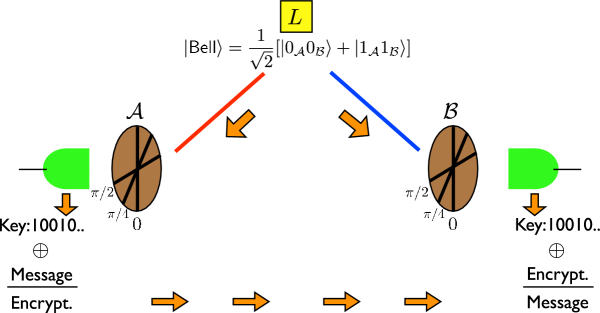
Figure 4.1: Quantum cryptographic protocol. A source $L$ emits pairs of maximally entangled photons. Alice and Bob measure their polarization in random bases and they only keep those measured in the same direction. In this way they build a key used to encrypt their message.

Although the scheme presented seems simple and successful, an eavesdropper could still hear the conversation by, for example, stealing entangled qubits used to build up the key. Many different cryptography protocols have been designed for different situations and can be found in the literature. Here I only discussed the basics of quantum cryptography to show that entangled states play an important role in information processes.

4.1.2 Quantum Teleportation

Quantum teleportation [BBC93] consists of the process of teleporting the state of a distant quantum system by means of local quantum operations, including measurements, and classical communication (LOCC). The simplest case considers the teleportation of the state of a single qubit. For this purpose assume that Alice possesses two qubits denoted by ${\cal A}_{1}$ and ${\cal A}_{2}$, and Bob possesses only one, denoted by $\cal B$. Moreover, assume that qubits ${\cal A}_{2}$ and $\cal B$ are in a maximally entangled state which was given by an external source. Such an entangled state can then be used to teleport the state of qubit ${\cal A}_{1}$ to qubit $\cal B$.

The idea is the following: The global three-qubit state of Alice and Bob together is given by $|{\psi}\rangle=(a|{0_{{\cal A}_{1}}}\rangle+b|{1_{{\cal A}_{1}}}\rangle)\otimes\frac{1}{\sqrt{2}}(|{0_{{\cal A}_{2}}0_{\cal B}}\rangle+|{1_{{\cal A}_{2}}1_{\cal B}}\rangle)$. This state can also be written as

$$|{\psi}\rangle=\frac{1}{2}\left[|{\phi^{+}}\rangle(a|{0_{\cal B}}\rangle+b|{1_{\cal B}}\rangle)+|{\phi^{-}}\rangle(a|{0_{\cal B}}\rangle-b|{1_{\cal B}}\rangle)+\right.$$ (4.1)

$$\left.|{\xi^{+}}\rangle(a|{1_{\cal B}}\rangle+b|{0_{\cal B}}\rangle)+|{\xi^{-}}\rangle(a|{1_{\cal B}}\rangle-b|{0_{\cal B}}\rangle)\right],$$

where Alice’s states $|{\phi^{\pm}}\rangle$ and $|{\xi^{\pm}}\rangle$ are the Bell states

$$|{\phi^{\pm}}\rangle = \frac{1}{\sqrt{2}}(|{0_{{\cal A}_{1}}0_{{\cal A}_{2}}}\rangle\pm|{1_{{\cal A}_{1}}1_{{\cal A}_{2}}}\rangle)\mbox{ and}$$ (4.2)

$$|{\xi^{\pm}}\rangle = \frac{1}{\sqrt{2}}(|{0_{{\cal A}_{1}}1_{{\cal A}_{2}}}\rangle\pm|{1_{{\cal A}_{1}}0_{{\cal A}_{2}}}\rangle),$$

respectively. Remarkably, in this basis (Eq. 4.2) the state of Bob’s qubit looks very similar to the state to be teleported (i.e., the state of ${\cal A}_{1}$). Then, Alice performs a measurement in her two qubits projecting them into one of the four possible Bell states. (Such a measurement can be done using local operations only but I do not describe it here.).

The state obtained by Alice corresponds to one of the four possibilities shown in Eq. 4.2. Alice then contacts Bob and tells him about the result of the measurement, after which Bob acts on its qubit to recover the state of ${\cal A}_{1}$. For example, if Alice projects its two-qubit state into $|{\xi^{+}}\rangle$, then she tells this result (by means of a classical communication) to Bob. He thereby transforms the state of his qubit by using a flip operation transforming

$$a|{1_{\cal B}}\rangle+b|{0_{\cal B}}\rangle\rightarrow a|{0_{\cal B}}\rangle+b|{1_{\cal B}}\rangle,$$ (4.3)

which is the desired teleported state. Similar operations can be done for any other state measured by Alice.

4.2 Quantum Entanglement and Quantum Computation

Perhaps the most important practical case where QE can be used as a resource is in computational tasks. As mentioned before, parallelism is one of the properties of the quantum world that needs to be exploited in a quantum computation, and such a property is naturally associated to QE. Shor’s factoring algorithm [Sho94] constitutes a nice example where entangled states are used to find the prime factors of a whole number. It has been shown that using a QC, this algorithm can be efficiently performed; that is, with a number of steps that scales at most polynomially with the integer $P$ to be factorized. However, it is not known how to perform such an algorithm efficiently on a CC: In order to find the factors of $P$ it is necessary to divide it by all the whole numbers between 1, and $P/2$, and so on, constituting a time consuming task.

To demonstrate Shor’s algorithm, I present the factorization of the number $P=15$. (Although the solution to this problem is immediately found, $P=15=3\times 5$, this method can be extended to the factorization of larger numbers like $P^{\prime}=12319$, where finding the solution is more complicated: $P^{\prime}=97\times 127$.) As I will show, the problem of finding the factors of $P$ is equivalent to the order-finding problem. Thus, a random whole number $m$ between 1 and $P-1$ needs to be chosen first. Assume that this number is $m=8$. Second, a QA needs to be performed to find the order $n$ of $m$, modulo $P$. Such order is defined as the least positive integer such that $m^{n}=1(\mbox{ mod }P)$, where $a=b(\mbox{ mod }P)$ if $a-b$ is divisible by $P$.

Then, the first step of the QA consists of performing $r$ Hadamard gates to the initial $(r+4)$-qubit polarized state $|{0_{1}\cdots 0_{r}}\rangle\otimes|{0_{a}0_{b}0_{c}0_{d}}\rangle$. The number $r$ of extra qubits has to be big enough to find the order $n$ with high accuracy [Sho94]. Here, $r=11$. The other 4 qubits are necessary to encode information about the factors of $15$ (i.e., $2^{4}=16>15$).

After the Hadamard gates have been applied (i.e., the gates that transform $|{0}\rangle\rightarrow|{+}\rangle$), the evolved state is

$$|{\psi}\rangle=\frac{1}{\sqrt{2^{r}}}\sum\limits_{j=0}^{2^{r}-1}|{j}\rangle\otimes|{0_{a}0_{b}0_{c}0_{d}}\rangle,$$ (4.4)

where $|{j}\rangle$ is the state corresponding to the binary decomposition of the integer $j$ in the logical basis; for example, $|{j=3}\rangle=|{0_{1}\cdots 1_{r-1}0_{r}}\rangle$. The next step of the algorithm is to apply a unitary operation that transforms

$$|{j}\rangle\otimes|{0_{a}0_{b}0_{c}0_{d}}\rangle\rightarrow|{j}\rangle\otimes|{m^{j}(\mbox{ mod }P)}\rangle.$$ (4.5)

This operation can be efficiently performed using controlled operations on the state of the $r$ qubits, but I will not explain it here. After this evolution, the evolved state is

$$|{\psi}\rangle = \frac{1}{\sqrt{2^{r}}}\sum\limits_{j=0}^{2^{r}-1}|{j}\rangle\otimes|{m^{j}(\mbox{ mod }P)}\rangle$$

$$= \frac{1}{\sqrt{2^{r}}}\left[|{0}\rangle\otimes|{1}\rangle+|{1}\rangle\otimes|{8}\rangle+|{2}\rangle\otimes|{4}\rangle+|{3}\rangle\otimes|{2}\rangle+\cdots\right],$$

where again I have chosen the integer representation of the states in the logical basis. The state of Eq. 4.2 is a highly entangled state between the $r=11$ qubits and qubits $a$, $b$, $c$, and $d$.

By defining the states $|{\mu_{q}}\rangle$ for qubits $a,b,c,d$, as

$$|{\mu_{q}}\rangle=\frac{1}{\sqrt{n}}\sum\limits_{k=0}^{n-1}\exp\left[\frac{-i2\pi qk}{n}\right]|{m^{k}(\mbox{ mod }P)}\rangle,$$ (4.7)

where again $n$ is the not yet known order, Eq. 4.2 can be written as

$$|{\psi}\rangle=\frac{1}{\sqrt{n2^{r}}}\sum\limits_{q=0}^{n-1}\sum\limits_{j=0}^{2^{r}-1}\exp\left[i\frac{2\pi qj}{n}\right]|{j}\rangle\otimes|{\mu_{q}}\rangle.$$ (4.8)

A (inverse) quantum Fourier transform [NC00] performed to the $r$ qubits in the above state maps it to

$$\frac{1}{\sqrt{2^{r}}}\sum\limits_{j=0}^{2^{r}-1}\exp\left[i\frac{2\pi qj}{n}\right]|{j}\rangle\rightarrow|{\overline{K=q/n}}\rangle,$$ (4.9)

where the state $|{\overline{K=q/n}}\rangle$ of the $r$ qubits is a product state which depends on the coefficient $q/n$ as in the usual Fourier transform. This transformation can also be efficiently implemented in a quantum circuit. Therefore, the transformed state reads

$$|{\psi}\rangle=\frac{1}{\sqrt{n}}\sum\limits_{q=0}^{n-1}|{\overline{K=q/n}}\rangle\otimes|{\mu_{q}}\rangle.$$ (4.10)

In this way, the register of $r$ qubits is measured in the logical basis to project the state $|{\psi}\rangle$ and obtain one possible state $|{\overline{K=q/n}}\rangle\otimes|{\mu_{q}}\rangle$. After applying the same algorithm several times and by applying a continued-fractions algorithm, it is possible to obtain the order $n$ from the statistics of the measured states $|{\overline{K=q/n}}\rangle$. In this case one would obtain $n=4$, such that $8^{4}=4096=1(\mbox{ mod }15)$. Such a solution could be obtained if the result of the measurement in the register of $r$ qubits gives, for example, $|{\overline{K=q/n}}\rangle=|{1536}\rangle$ (in the binary representation), where I have used again the integer representation of states in the logical basis. If this is the case, $q/n=\frac{1536}{2^{11}}=\frac{3}{4}$, resulting in $n=4$. From this information, one can obtain that $15=3\times 5$ as it is explained in Ref. [Sho94].

A factoring QA such as the one presented is more efficient than a classical one only because entangled states have been created at some step. Otherwise, no advantages can be gained, in general, from using a deterministic QC. As a simple example, suppose (with no loss of generality) that the initial pure state of a register of $N$ qubits is the usual polarized state $|{0_{1}\cdots 0_{N}}\rangle$, and that the QA never does create QE. That is, the set of unitary gates $U_{j}$ applied to the initial state are only single qubit rotations transforming product states into product states. Therefore,

$$U_{j}=e^{i\theta_{j}\sigma^{\alpha(j)}_{\pi(j)}}=\cos\theta+i\sin\theta\sigma^{\alpha(j)}_{\pi(j)},$$ (4.11)

where $\pi(j)=[1\cdots N]$ denotes the qubit rotated at the $j$th step, and $\alpha(j)=[x,y,z]$ is the axis of rotation. The evolved state is then

$$\prod_{j}U_{j}|{0_{1}\cdots 0_{N}}\rangle.$$ (4.12)

After the evolution is performed, certain qubit(s) is(are) measured in, for example, the logical basis. As usual, this is the last step of a deterministic QA (Sec. 2.2). If the $k$th qubit is measured, the result obtained is

$$\langle\sigma_{z}^{k}\rangle=\langle{0_{1}\cdots 0_{N}}|\left(\prod_{j}U^{\dagger}_{j}\right)\sigma_{z}^{k}\left(\prod_{j}U_{j}\right)|{0_{1}\cdots 0_{N}}\rangle.$$ (4.13)

The fact is that such QA can be simulated classically and the expectation value of Eq. 4.13 can be computed in a CC with the same amount of resources (i.e., same efficiency). The idea is to only keep track of the information about $[\theta_{j},\alpha(j)]$ if $\pi(j)=k$, because the other qubits are not measured. If the QA is performed efficiently, only a polynomially large number of pairs $[\theta_{j},\alpha(j)]$ are kept. A classical algorithm to obtain the result of Eq. 4.13 would consist of updating at each step the state of the $k$th qubit only. For example, if at the $j$th step the state is $a_{j}|{0_{k}}\rangle+b_{j}|{1_{k}}\rangle$ and the gate $U_{j+1}=e^{i\frac{\pi}{4}\sigma_{x}^{k}}$ is performed after, the evolved state becomes

$$[\cos(\pi/4)+i\sin(\pi/4)\sigma_{x}^{k}](a_{j}|{0_{k}}\rangle+b_{j}|{1_{k}}\rangle)=a_{j+1}|{0_{k}}\rangle+b_{j+1}|{1_{k}}\rangle,$$ (4.14)

and since $\sigma_{x}^{k}$ is the corresponding flip operation, $a_{j+1}=\frac{1}{\sqrt{2}}(a_{j}+ib_{j})$ and $b_{j+1}=\frac{1}{\sqrt{2}}(ia_{j}+b_{j})$. Updating the values of the complex coefficients $a_{j}$ and $b_{j}$ can be easily done with a conventional computer. At the end of the total evolution the state of the $k$th qubit is $a_{M}|{0_{k}}\rangle+b_{M}|{1_{k}}\rangle$. Therefore, the result of Eq. 4.13 is

$$\langle\sigma_{z}^{k}\rangle=|a_{M}|^{2}-|b_{M}|^{2},$$ (4.15)

which can be efficiently computed with a CC.

However, if some of the gates $U_{j}$ create entanglement, there is no known way, in general, to classically evaluate Eq. 4.13 efficiently. Naturally, the elementary two-qubit gates, like the $R_{z^{j}z^{k}}(\omega)$ or the CNOT gate introduced in Sec. 2.1.3, are responsible for creating entanglement. For example, if the initial state is the product (unentangled) state $\frac{1}{\sqrt{2}}|{0+1}\rangle\otimes|{0}\rangle$, applying the CNOT gate evolves it into $\frac{1}{\sqrt{2}}(|{00}\rangle+|{11}\rangle)$, which is known to be one of the Bell states, that is, maximally entangled. Nonetheless, I will show in the next section that creation of QE is not a sufficient condition to claim that Eq. 4.13 cannot be obtained efficiently by using a classical algorithm.

4.3 Efficient Classical Simulations of Quantum Physics

The purpose of this section is to generalize the concepts described previously, presenting a wide set of problems which can be solved efficiently with both, a QC or a classical one. To show this, I will exploit the notion of GE, which was presented in Sec. 3.2. Again, an algorithm is said to be efficient with respect to a certain variable $N$, whenever the amount of resources required to perform it is bounded by a polynomial in $N$. Otherwise, the algorithm is said to be inefficient. It is important to remark that here I only make a comparison between efficient and inefficient algorithms, with the previous definition, and do not compare the total amount of resources needed. For example, if a QA can be performed in $N$ operations and the corresponding classical one in $N^{2}$ operations then, despite being more convenient to use the former, both are considered efficient.

In most cases, the type of problems one encounters in quantum mechanics are related with the evaluation of a certain expectation value or correlation function

$$\langle\hat{W}\rangle=\langle{\phi}|\hat{W}|{\phi}\rangle,$$ (4.16)

where $\hat{W}$ is an operator acting on a finite quantum system ${\cal S}$ in some state $|{\phi}\rangle\in\cal H$. ($\cal H$ is the Hilbert space associated to $\cal S$.) In Sec. 2.2, I presented some QAs that allow one to compute Eq. 4.16 in a QC described by the conventional model, whenever the operator algebra associated to the system $\cal S$ could be mapped onto the Pauli operators (Sec. 2.3). The main steps of those QAs consist of the preparation of the state $|{\psi}\rangle=|{+}\rangle_{\sf a}\otimes|{\phi}\rangle$, from some initial (boot-up) reference state like $|{0}\rangle_{\sf a}\otimes|{0\cdots 0}\rangle$, then an evolution, and finally the measurement of the ancilla qubit ${\sf a}$. Similarly, in the rest of this section I assume that the algebra of operators used to describe the quantum computational model and/or the algebra associated to the system $\cal S$ are not necessarily described by the conventional model, but a one-to-one efficient mapping between both exists.

Since I am mainly interested in comparing the efficiencies of obtaining Eq. 4.16 using a QC or a classical (conventional) one, the efficiency is defined relative to a certain variable $N$ which here is, in general, the number of quantum mechanical elements that compose the system $\cal S$. I assume that there exists a QA that evaluates Eq. 4.16 efficiently, that is, using at most $\mbox{poly}(N)$ resources. These are the so-called bounded polynomial quantum algorithms (BPQA). This is usually valid whenever the QC can be efficiently initialized and every step, including the preparation of $|{\phi}\rangle$, can be efficiently performed. These results were previously discussed in Sec. 2.5.

The most common classical algorithm to evaluate Eq. 4.16 consists of writing the matrix representation of $\hat{W}$, and obtaining the corresponding matrix element. This is usually a hard task because of the dimension of the Hilbert space $\cal H$ growing exponentially with $N$. However, in some cases this complexity can be highly reduced. The simplest case is when the state $|{\phi}\rangle$ of Eq. 4.16 is known to be an eigenstate of $\hat{W}$, so that the corresponding expectation is simply the known eigenvalue.

Nonetheless, a more general result can be obtained in a Lie algebraic framework. For this purpose, I start by pointing out that, with no loss of generality, the state $|{\phi}\rangle\in\cal H$ of Eq. 4.16 can be obtained by transforming any reference state $|{\sf ref}\rangle\in\cal H$; that is

$$|{\phi}\rangle=U|{\sf ref}\rangle,$$ (4.17)

where $U^{\dagger}=U^{-1}$ (unitary). Moreover, the reference state can be chosen to be the highest (or lowest) weight state $|{\sf HW}\rangle$ of certain finite semi-simple Lie algebra $\mathfrak{h}=\{\hat{O}_{1},\hat{O}_{2},\cdots,\hat{O}_{M}\}$, with $\hat{O}_{j}=\hat{O}_{j}^{\dagger}$ (Sec. 3.2.2). In this case, $\mathfrak{h}$ also admits a Cartan-Weyl decomposition: $\mathfrak{h}=\{\mathfrak{h}_{D},\mathfrak{h}_{+},\mathfrak{h}_{-}\}$, with $\mathfrak{h}_{D}$ the Cartan subalgebra (CSA) of $\mathfrak{h}$, and $\mathfrak{h}_{+}$ and $\mathfrak{h}_{-}$ the set of raising and lowering operators, respectively (Sec. 3.2.2).

Now suppose that the transformation $U$ of Eq. 4.17 is a group operation induced by $\mathfrak{h}$; that is

$$U=\exp\left[i\sum\limits_{j=1}^{M}\zeta_{j}\hat{O}_{j}\right].$$ (4.18)

Then $|{\psi}\rangle$ is a GCS and generalized unentangled state (extremal) of $\mathfrak{h}$. Moreover, suppose that $\hat{W}$ of Eq. 4.16 can be decomposed as

$$\hat{W}=\sum\limits_{j=1}^{M}\kappa_{j}\hat{O}_{j},$$ (4.19)

where $\kappa_{j}\in\mathbb{C}\ \forall j$, and $\hat{O}_{j}\in\mathfrak{h}$. In general, $\hat{W}$ does not have the form of Eq. 4.19 and it belongs to a Lie algebra other than $\mathfrak{h}$. Then, $\mathfrak{h}$ must be considered as the Lie algebra that contains both. (The important case when $\hat{W}\in H\equiv e^{i\mathfrak{h}}$, i.e. the group induced by $\mathfrak{h}$, is discussed in the next section.)

In this way, computing classically Eq. 4.16 is equivalent to evaluating

$$\langle\hat{W}\rangle=\sum\limits_{j=1}^{M}\kappa_{j}\langle{\sf HW}|e^{-i\sum\limits_{j=1}^{M}\zeta_{j}\hat{O}_{j}}\hat{O}_{j}e^{i\sum\limits_{j=1}^{M}\zeta_{j}\hat{O}_{j}}|{\sf HW}\rangle.$$ (4.20)

The operators

$$\hat{O}^{\prime}_{j}=e^{-i\sum\limits_{j=1}^{M}\zeta_{j}\hat{O}_{j}}\hat{O}_{j}e^{i\sum\limits_{j=1}^{M}\zeta_{j}\hat{O}_{j}}=\sum\limits_{j^{\prime}=1}^{M}\nu_{jj^{\prime}}\hat{O}_{j^{\prime}}$$ (4.21)

are also elements in $\mathfrak{h}$ because they are transformed by a group operation. The coefficients $\nu_{jj^{\prime}}$ of Eq. 4.21 can be computed by means of the representation theory. A matrix representation of $\mathfrak{h}$ is the mapping $\Phi:\mathfrak{h}\rightarrow\mathbb{C}^{2p}$ such that

$$\Phi(\hat{O}_{j}) = \bar{O}_{j},$$ (4.22)

$$\Phi([\hat{O}_{j},\hat{O}_{j^{\prime}}]) = \left[\Phi(\hat{O}_{j}),\Phi(\hat{O}_{j^{\prime}})\right]=\left[\bar{O}_{j},\bar{O}_{j^{\prime}}\right],$$

where $[A,B]$ is the commutator and the complex matrices $\bar{O}_{j}$ are $p\times p$ dimensional. A representation $\Phi$ is said to be faithful when maps linearly independent elements in $\mathfrak{h}$ to linearly independent $p\times p$ matrices. If the Lie algebra $\mathfrak{h}$ is compact, one can always find a faithful representation satisfying the inner product

$${\sf Tr}[\bar{O}_{j}\bar{O}_{j^{\prime}}]=\delta_{jj^{\prime}},$$ (4.23)

with ${\sf Tr}[\bar{Q}]$ being the trace of $\bar{Q}$. For example, the well known adjoint representation (Appendix C), which associates an $M\times M$ matrix to every operator in $\mathfrak{h}$ ($M$ is the dimension of $\mathfrak{h}$), is faithful and satisfies Eq. 4.23. Nevertheless, smaller dimensional faithful representations ($p<M$) can usually be found. Then, if $\Phi$ is faithful,

$$\bar{O}^{\prime}_{j}=e^{-i\sum\limits_{j=1}^{M}\zeta_{j}\bar{O}_{j}}\bar{O}_{j}e^{i\sum\limits_{j=1}^{M}\zeta_{j}\bar{O}_{j}}=\sum\limits_{j^{\prime}=1}^{M}\nu_{jj^{\prime}}\bar{O}_{j^{\prime}},$$ (4.24)

which is the matrix representation of Eq. 4.21. Since this is a matrix operation, the matrices $\bar{O}^{\prime}_{j}$ of Eq. 4.24 can be classically computed with ${\cal O}(p^{2})$ computational operations (addition and multiplication of complex numbers). Each coefficient $\nu_{jj^{\prime}}$ is then classically obtained by using the inner product equation, that is

$$\nu_{jj^{\prime}}={\sf Tr}[\bar{O}^{\prime}_{j}\bar{O}_{j^{\prime}}],$$ (4.25)

which also requires ${\cal O}(p^{2})$ computational operations.

Similarly, in the CW basis,

$$\hat{O}^{\prime}_{j}=\sum\limits_{k=1}^{r}\gamma_{jk}\hat{h}_{k}+\sum\limits_{j^{\prime}=1}^{l}\iota_{jj^{\prime}}\hat{E}_{\alpha_{j^{\prime}}}+\iota_{jj^{\prime}}^{*}\hat{E}_{-\alpha_{j^{\prime}}}\,$$ (4.26)

where $\hat{h}_{k}\in\mathfrak{h}_{D}$ (CSA), $E_{\alpha_{j^{\prime}}}\in\mathfrak{h}_{+}$, and $E_{-\alpha_{j^{\prime}}}\in\mathfrak{h}_{-}$ (Sec. 3.2.2). The coefficients $\gamma_{jk}$ and $\iota_{jj^{\prime}}$ of Eq. 4.26 can also be obtained classically with ${\cal O}(p^{2})$ computational operations by the trace inner product: The operators $\hat{h}_{k}$, $\hat{E}_{\alpha_{j^{\prime}}}$, and $\hat{E}_{-\alpha_{j^{\prime}}}$ are usually a simple linear combinations of the operators $\hat{O}_{j}$.

By definition, $|{\sf HW}\rangle$ is an eigenstate of the operators in the CSA, that is

$$\hat{h}_{k}|{\sf HW}\rangle=e_{k}|{\sf HW}\rangle,$$ (4.27)

where the eigenvalues $e_{k}$ are assumed to be known. Then,

$$\langle{\sf HW}|\hat{E}_{\alpha_{j^{\prime}}}|{\sf HW}\rangle=\langle{\sf HW}|\hat{E}_{-\alpha_{j^{\prime}}}|{\sf HW}\rangle=0\ \ \forall j^{\prime}.$$ (4.28)

In other words, Eq. 4.20 can be classically computed by only keeping the elements of $\hat{O}^{\prime}_{j}$ (Eq. 4.21) belonging to $\mathfrak{h}_{D}$:

$$\langle{{\sf HW}}|\hat{O}^{\prime}_{j}|{{\sf HW}}\rangle=\sum\limits_{k=1}^{r}\gamma_{jk}\langle{\sf HW}|\hat{h}_{k}|{\sf HW}\rangle=\sum\limits_{k=1}^{r}\gamma_{jk}e_{k},$$ (4.29)

and

$$\langle\hat{W}\rangle=\sum\limits_{j=1}^{M}\sum\limits_{k=1}^{r}\kappa_{j}\gamma_{jk}e_{k}.$$ (4.30)

Since the coefficients $e_{k}$ are assumed to be known, and the coefficients $\kappa_{j}$ and $\gamma_{jk}$ can be classically obtained with ${\cal O}(p^{2})$, Eq. 4.30 can be computed with ${\cal O}(Mrp^{2})$ computational operations. If $M\leq\mbox{poly}(N)$, then $r\leq\mbox{poly}(N)$. Also, the existence of the adjoint representation (Appendix C) guarantees that one can always find $p$ such that $p\leq M\leq\mbox{poly}(N)$. Therefore, Eq. 4.30 can be efficiently computed with a conventional computer. A more detailed proof about the number of operations required, including the approximation of the exponential matrix, is given in the Appendix E.

In brief, when the state $|{\phi}\rangle$ of Eq. 4.16 is a GCS of a polynomially large dimensional Lie algebra $\mathfrak{h}$, and the operator $\hat{W}$ is an element of $\mathfrak{h}$, Eq. 4.16 can be efficiently computed with both, a classical and a quantum device.

However, in some cases $\hat{W}$ or $U$ (Eq. 4.17) are associated with an exponentially large dimensional Lie algebra and the corresponding classical simulation is inefficient. Nevertheless, it is important to remark that for mixed states of the form

$$\rho=\sum\limits_{s=1}^{L}p_{s}\rho_{s},$$ (4.31)

where $\rho_{s}=|{\phi_{s}}\rangle\langle{\phi_{s}}|$, and $|{\phi_{s}}\rangle$ being GCSs and generalized unentangled states of a polynomially large dimensional Lie algebra, the computation of

$$\langle\hat{W}\rangle={\sf Tr}(\rho\hat{W}),$$ (4.32)

can also be efficiently performed with a CC if $L\leq\mbox{poly}(N)$.

4.3.1 Higher Order Correlations

The previous results can be extended to the computation of higher order correlations. For simplicity, I start by studying the case of two-body correlations of the form

$$\langle\hat{W}\rangle=\langle{\phi}|\hat{W}_{1}\hat{W}_{2}|{\phi}\rangle,$$ (4.33)

where $\hat{W}$ is the product of the observables $\hat{W}_{1}=\hat{W}_{1}^{\dagger}$ and $\hat{W}_{2}=\hat{W}_{2}^{\dagger}$. Again, $\hat{W}_{1}$ and $\hat{W}_{2}$ are considered to be elements of a Lie algebra $\mathfrak{h}=\{\hat{O}_{1},\cdots,\hat{O}_{M}\}$, and $|{\phi}\rangle$ is assumed to be a GCS of $\mathfrak{h}$; that is

$$|{\phi}\rangle=U|{\sf HW}\rangle,$$ (4.34)

with $U=\exp\left[i\sum_{j}\zeta_{j}\hat{O}_{j}\right]$, and $|{\sf HW}\rangle$ the highest weight state of $\mathfrak{h}$. In this way, Eq. 4.33 reads

$$\langle{\phi}|\hat{W}_{1}\hat{W}_{2}|{\phi}\rangle=\langle{\sf HW}|U^{\dagger}\hat{W}_{1}\hat{W}_{2}U|{\sf HW}\rangle.$$ (4.35)

Since $UU^{\dagger}={\mathchoice{\rm 1\mskip-4.0mul}{\rm 1\mskip-4.0mul}{\rm 1\mskip-4.5mul}{\rm 1\mskip-5.0mul}}$,

$$\langle{\phi}|\hat{W}_{1}\hat{W}_{2}|{\phi}\rangle=\langle{\sf HW}|\hat{W}^{\prime}_{1}\hat{W}^{\prime}_{2}|{\sf HW}\rangle,$$ (4.36)

where $\hat{W}^{\prime}_{i}=U^{\dagger}\hat{W}_{i}U$.

Equation 4.33 can be efficiently computed with a classical computer if the dimension $M$ of $\mathfrak{h}$ scales at most polynomially with the variable $N$; i.e. $M\leq\mbox{poly}(N)$. To show this, I first decompose the corresponding operators as

$$\hat{W}_{1}=\sum\limits_{j=1}^{M}\kappa^{1}_{j}\hat{O}_{j},$$ (4.37)

$$\hat{W}_{2}=\sum\limits_{j=1}^{M}\kappa^{2}_{j}\hat{O}_{j},$$ (4.38)

which transform under the action of $U$ as

$$\hat{W}^{\prime}_{i}=U^{\dagger}\hat{W}_{i}U=\sum_{j=1}^{M}\kappa^{i}_{j}\hat{O}^{\prime}_{j}\ ;\ i=1,2.$$ (4.39)

In a CW basis of $\mathfrak{h}$, the transformed observables $\hat{O}^{\prime}_{j}=U^{\dagger}\hat{O}_{j}U$ can be decomposed as in Eq. 4.26. Such decomposition can be done efficiently with a CC (i.e., computing the coefficients $\gamma_{jk}$ and $\iota_{jj^{\prime}}$) by working in low-dimensional faithful representation of $\mathfrak{h}$ (Appendix C). Then,

$$\langle\hat{W}_{1}\hat{W}_{2}\rangle=\sum\limits_{i,j=1}^{M}\kappa_{i}^{1}\kappa_{j}^{2}\langle{\sf HW}|\hat{O}^{\prime}_{i}\hat{O}^{\prime}_{j}|{\sf HW}\rangle,$$ (4.40)

with

$$\langle{\sf HW}|\hat{O}^{\prime}_{i}\hat{O}^{\prime}_{j}| {\sf HW}\rangle=\sum\limits_{k,k^{\prime}=1}^{r}\gamma_{ik}\gamma_{jk^{\prime}}\langle\hat{h}_{k}\hat{h}_{k^{\prime}}\rangle+\sum\limits_{i^{\prime},j^{\prime}=1}^{l}\left[\iota_{ii^{\prime}}\iota_{jj^{\prime}}\langle\hat{E}_{\alpha_{i^{\prime}}}\hat{E}_{\alpha_{j^{\prime}}}\rangle\right.$$ (4.41)

$$+\left.\mbox{C.C.}+\iota_{ii^{\prime}}\iota^{*}_{jj^{\prime}}\langle\hat{E}_{\alpha_{i^{\prime}}}\hat{E}_{-\alpha_{j^{\prime}}}\rangle+\iota^{*}_{ii^{\prime}}\iota_{jj^{\prime}}\langle\hat{E}_{-\alpha_{i^{\prime}}}\hat{E}_{\alpha_{j^{\prime}}}\rangle\right]$$

$$+\sum\limits_{k=1}^{r}\sum\limits_{j^{\prime}=1}^{l}\left[\gamma_{ik}\iota_{jj^{\prime}}\langle\hat{h}_{k}\hat{E}_{\alpha_{j^{\prime}}}\rangle+\gamma_{ik}\iota^{*}_{jj^{\prime}}\langle\hat{h}_{k}\hat{E}_{-\alpha_{j^{\prime}}}\rangle+\mbox{C.C.}\right],$$

where C.C. denotes the complex conjugate, and the expectation values are now taken over the highest weight state, i.e. $\langle\hat{A}\rangle=\langle{\sf HW}|\hat{A}|{\sf HW}\rangle$. Since raising operators annihilate $|{\sf HW}\rangle$ only a few expectations do not vanish in Eq. 4.41. These are

$$\langle\hat{h}_{k}\hat{h}_{k^{\prime}}\rangle = e_{k}e_{k^{\prime}},$$ (4.42)

$$\langle E_{\alpha_{j^{\prime}}}E_{-\alpha_{j^{\prime}}}\rangle = \langle E_{-\alpha_{j^{\prime}}}E_{\alpha_{j^{\prime}}}+\sum\limits_{k=1}^{r}\alpha_{j^{\prime}}^{k}\hat{h}_{k}\rangle=\sum\limits_{k=1}^{r}\alpha_{j^{\prime}}^{k}e_{k},$$ (4.43)

where the coefficients $\alpha_{j}^{k}$ are the components of the root vector $\alpha_{j}$ (Sec. 3.2.2) and $e_{k}$ are the known weights of $|{\sf HW}\rangle$.

In brief, Eq. 4.33 takes the form

$$\langle{\phi}|\hat{W}_{1}\hat{W}_{2}|{\phi}\rangle=\sum\limits_{i,j=1}^{M}\kappa_{i}^{1}\kappa_{j}^{2}\left[\sum\limits_{k,k^{\prime}=1}^{r}\gamma_{ik}\gamma_{jk^{\prime}}e_{k}e_{k^{\prime}}+\sum\limits_{j^{\prime}=1}^{l}\sum\limits_{k=1}^{r}\iota_{ij^{\prime}}\iota^{*}_{jj^{\prime}}\alpha_{j^{\prime}}^{k}e_{k}\right],$$ (4.44)

which can be efficiently computed with a CC if $M\leq\mbox{poly}(N)$.

Higher order correlation functions of the form

$$\langle\hat{W}\rangle=\langle{\phi}|\hat{W}^{p}\cdots\hat{W}^{1}|{\phi}\rangle$$ (4.45)

can also be computed efficiently for a fixed integer $R$, whenever there is a polynomially large dimensional Lie algebra $\mathfrak{h}$ associated to the problem. Obviously, the complexity of this problem increases as $p$ does. Again, the idea is to keep only the nonzero expectations of the transformed operator $\hat{W}^{\prime}=U^{\dagger}\hat{W}^{p}\cdots\hat{W}^{1}U=\hat{W}^{\prime p}\cdots\hat{W}^{\prime 1}$, where $|{\phi}\rangle=U|{\sf HW}\rangle$. For this purpose, all the raising operators $\hat{E}_{\alpha_{j}}$ appearing in $\hat{W}^{\prime}$ must be taken to the right side, by using the commutation relations of the algebra, so that they destroy the state $|{\sf HW}\rangle$. This problem is analogous to the one given by Wick’s theorem [Wic50] for fermionic operators. In Appendix F, I describe an efficient method for the classical computation of Eq. 4.45.

4.4 Generalized Entanglement and Quantum Computation

In Sec. 4.3 I presented a class of classical algorithms that allows one to efficiently obtain certain correlation functions of quantum systems in a conventional computer. Here, I analyze some advantages of having a QC. For example, assume then that one is interested in the evaluation of the correlation function of Eq. 4.16, when there is no polynomially large dimensional Lie algebra $\mathfrak{h}$ associated with the problem. That is, either $|{\phi}\rangle$ is not a GCS of $\mathfrak{h}$ or $\hat{W}$ is not an element or group element induced by $\mathfrak{h}$. Then, if a bounded polynomial quantum algorithm (BPQA) like the ones introduced in Sec. 2.2 exists in this case, Eq. 4.16 can be efficiently computed using a QC. Usually, no known classical algorithm can be used to compute such a correlation efficiently and this represents, in some cases, an exponential speed-up of the quantum simulation with respect to the classical one.

In Sec. 2.5, I discussed the complexity of simulating physical systems using QCs. Although certain QSs have been shown to be efficient, others, like the obtention of the ground state properties in the two-dimensional Hubbard model, remained inefficient. The problem relied in the complexity of preparing the desired initial state $|{\phi}\rangle$. When simulating quantum systems, this state is usually not completely known (e.g., it is the ground state of some non-solvable Hamiltonian) and an approximated state, having a non-zero overlap with $|{\phi}\rangle$, needs to be prepared. The purpose of the following section is then to show a wide class of quantum states that can be prepared efficiently by quantum networks. Again, the results obtained are independent of the physical representation of the QC whenever an efficient mapping between the operators used to describe the system to be simulated and the operators describing the computational model, exists.

4.4.1 Efficient Initial State Preparation

I start by describing the simple case when the initial state to be prepared is given by

$$|{\phi}\rangle=U|{\sf HW}\rangle,$$ (4.46)

where $|{\sf HW}\rangle$ is the highest weight of some Lie algebra $\mathfrak{h}$, and is considered to be the boot-up state of the computer, which can be efficiently initialized. If the operator $U$ of Eq. 4.46 is a group operation induced by $\mathfrak{h}$, that is, $U=e^{i\hat{A}}$ and $\hat{A}\in\mathfrak{h}=\{\hat{O}_{1},\cdots,\hat{O}_{M}\}$, and $M\leq\mbox{poly}(N)$, then $|{\phi}\rangle$ can be prepared efficiently with arbitrary accuracy by using, for example, a first order Trotter decomposition [Suz93]. In this case, the state $|{\phi}\rangle$ is generalized unentangled and GCS of $\mathfrak{h}$. Then, $\hat{A}=\sum_{j=1}^{M}\zeta_{j}\hat{O}_{j}$ and

$$e^{i\hat{A}}=\prod e^{i\hat{A}\Delta t},$$ (4.47)

$$e^{i\hat{A}\Delta t}\approx\prod\limits_{j=1}^{M}e^{i\zeta_{j}\hat{O}_{j}\Delta t}.$$ (4.48)

Assuming that every operation $e^{i\zeta_{j}\hat{O}_{j}\Delta t}$ is either an elementary gate or can be performed by applying a small number of them, the evolution $e^{i\hat{A}}$ can be then approximated by applying a polynomially large number of these gates. Particular examples were discussed in Sec. 2.3.

Another interesting case is when the state $|{\phi}\rangle$ is not given in the form of Eq. 4.46 but some information, like the expectation values of a set of observables (i.e., its reduced state), $\langle\hat{O}_{j}\rangle$, is known or can be easily obtained. If $\mathfrak{h}=\{\hat{O}_{1},\cdots,\hat{O}_{M}\}$ is a semi-simple Lie algebra, with $M\leq\mbox{poly}(N)$, and $|{\phi}\rangle$ is shown to be a GCS of $\mathfrak{h}$ by calculating, for example, the $\mathfrak{h}$-purity (Sec. 3.2.2), then it can be prepared efficiently with a QC. To show this, one needs to obtain first the operator $\hat{A}=\sum_{j=1}^{M}\zeta_{j}\hat{O}_{j}$ such that $U=e^{i\hat{A}}$ is the transformation of Eq. 4.46.

For this purpose, I define the fictitious Hamiltonian

$$H_{F}=-\sum\limits_{j=1}^{M}\langle\hat{O}_{j}\rangle\hat{O}_{j},$$ (4.49)

whose expectation value over the state $|{\psi}\rangle$ is

$$\langle{\psi}|H_{F}|{\psi}\rangle=-\sum\limits_{j=1}^{M}\langle\hat{O}_{j}\rangle^{2}.$$ (4.50)

If $|{\tilde{\psi}}\rangle=V|{\psi}\rangle$ is another GCS of $\mathfrak{h}$, with $V$ a unitary group operation that transforms as

$$V^{\dagger}\hat{O}_{j}V=\sum_{j^{\prime}=1}^{M}\nu_{jj^{\prime}}\hat{O}_{j^{\prime}},$$ (4.51)

then

$$\langle{\tilde{\psi}}|H_{F}|{\tilde{\psi}}\rangle=-\sum\limits_{j,j^{\prime}=1}^{M}\langle\hat{O}_{j}\rangle\nu_{jj^{\prime}}\langle\hat{O}_{j^{\prime}}\rangle.$$ (4.52)

Since the $M\times M$ matrix defined by the real coefficients $\nu_{jj^{\prime}}$ is orthogonal, one obtains (Schur’s inequality)

$$\langle{\tilde{\psi}}|H_{F}|{\tilde{\psi}}\rangle\geq\langle{\psi}|H_{F}|{\psi}\rangle.$$ (4.53)

Therefore, $|{\psi}\rangle$ is the unique GCS and ground state that minimizes such expectation value.

Assume now that $H_{F}$ can be efficiently diagonalized with a conventional computer, obtaining

$$H_{F}=UH_{0}U^{\dagger},$$ (4.54)

where $U$ is a unitary group operation and

$$H_{0}=\sum\limits_{k=1}^{r}\gamma_{k}\hat{h}_{k}\ ,$$ (4.55)

is an unperturbed Hamiltonian (i.e., $\hat{h}_{k}$ are elements in the CSA of $\mathfrak{h}$). Such a diagonalization algorithm is described in Sec. 5.2.1. Defining $|{\bar{\psi}}\rangle=U^{\dagger}|{\psi}\rangle$, one obtains

$$\langle{\psi}|H_{F}|{\psi}\rangle=\langle{\bar{\psi}}|H_{0}|{\bar{\psi}}\rangle,$$ (4.56)

which takes its minimum value, by definition, for a certain weight state $|{\phi}\rangle$. In particular, the coefficients $\gamma_{k}$ of Eq. 4.55 can be chosen such that $|{\bar{\psi}}\rangle=|{\sf HW}\rangle$ (see Chap. 5). Therefore, $|{\psi}\rangle=U|{\sf HW}\rangle$, and $U$ is the desired group operation. Again, $U$ can be approximated by applying a polynomially large number of elementary gates so $|{\psi}\rangle$ can be prepared efficiently with a QC.

4.5 Summary

In this chapter I have addressed several issues relating the concept of GE with quantum and classical complexity. I have shown that the creation of GE relative to every polynomially large dimensional Lie algebra is a necessary requirement to gain efficiency over the known classical algorithms. Otherwise, efficient classical simulations exist, which realize the computation by working in low-dimensional representations of the algebra. This result goes beyond the requirement of creating entangled states in the usual sense. For example, a quantum algorithm involving gates induced by the Lie algebra $\mathfrak{h}=\mathfrak{so}(2N)$, which is presented in detail in the next chapter, creates entangled states in the standard sense (i.e., non-separable). However, since the dimension of $\mathfrak{h}$ is polynomially large, such quantum computation can be efficiently simulated with a CC.

The efficient preparation of a wide class of states by quantum networks has also been studied. Again, any GCS or generalized unentangled state of a polynomially large dimensional Lie algebra can be efficiently prepared on a QC.

Chapter 5 Generalized Entanglement and Many-Body Physics

Information is inevitably physical.

Rolf Landauer

Every QC has associated certain physical representation (e.g., spin-1/2 system, etc.). The fact that information is not just an abstract entity and is always linked to a physical system, implies that it must be governed by the laws of physics. In Quantum Information Theory, for example, the manipulation and control of information is based on the foundations and laws of the quantum mechanics. On the other hand, many concepts, such as QE, have been developed only from an information-theory point of view. It is expected then that these concepts are also useful for the analysis of physical phenomena. In this chapter, I apply the notion of GE (Chap. 3) to the study of different problems in many-body physics.

First, I will focus on the characterization of quantum phase transitions (QPTs) in matter. QPTs are qualitative changes occurring in the properties of the ground state of a many-body system due to modifications either in the interactions among its constituents or in their interactions with an external probe [Sac99], while the system remains at zero temperature. Typically, such changes are induced as a parameter $g$ in the system Hamiltonian $H(g)$ is varied across a point at which the transition is made from one quantum phase to a different one. Often some correlation length diverges at this point, in which case the latter is called a quantum critical point. Because thermal fluctuations are inhibited, QPTs are purely driven by quantum fluctuations. Thus, these are purely quantum phenomena: A classical system in a pure state cannot exhibit quantum correlations. Prominent examples of QPTs are the quantum paramagnet to ferromagnet transition occurring in Ising spin systems under an external transverse magnetic field [LSM61, Pfe70, BM71], the superconductor to insulator transition in high-$T_{c}$ superconducting systems, and the superfluid to Mott insulator transition originally predicted for liquid helium and recently observed in ultracold atomic gases [GME02].

Since entanglement is a property inherent to quantum states and intimately related to quantum correlations (Chap. 3), one would expect that, in some appropriately defined sense, the entanglement present in the ground state undergoes a substantial change across a point where a QPT occurs. Thus, the concept of GE becomes specially well suited for this study because it is directly applicable to any algebraic language associated to the system under study.

Another important problem in quantum mechanics is to exactly diagonalize and obtain the spectrum of a Hamiltonian of a many-body system. In this case, no approximate methods (e.g., mean field theory) are needed and one has complete knowledge of the physical properties of the system through algebraic methods. By using information-theory concepts such as the ones described for the efficient simulation of physical systems (Sec. 4.3), I will show that whenever there is a Lie algebraic structure behind a problem in quantum physics, and the dimension of the associated Lie algebra is small enough, such problems can be solved easily by using a CC. This constitutes the final part of my thesis after which come the conclusions (Chap. 6).

5.1 Entanglement and Quantum Phase Transitions

In this section, I characterize the QPTs present in the Lipkin-Meshkov-Glick (LMG) model and in the anisotropic XY model in an external magnetic field through the GE notion, relative to a particular subset of observables which will be appropriately chosen in each case. Interestingly, for both of these models the ground states can be computed exactly by mapping the set of observable operators involved in the system Hamiltonian to a new set of operators which satisfy the same commutation relations; thus, preserving the underlying algebraic structure. In the new operator language, the models are seen to contain some symmetries that make them exactly solvable, allowing one to obtain the ground state properties in a number of operations that scales polynomially with the system size. It is possible then to understand which quantum correlations give rise to the QPTs in these cases.

Several issues should be considered when looking for an algebra $\mathfrak{h}$ of observables that may make the corresponding relative purity a good indicator of a QPT. First, one observes that in each of these cases a preferred Lie algebra exists, where the respective ground state would have maximum $\mathfrak{h}$-purity independently of the interaction strengths in the Hamiltonian. The purity relative to such an algebra remains constant, therefore it does not identify the QPT. (In these cases, this algebra is in fact the Lie algebra generated by the parametrized family of model Hamiltonians, as the parameters are varied.) Thus, one needs to extract a subalgebra relative to which the ground state may be generalized entangled, depending on the parameters in the Hamiltonian. A second, closely related observation is that the purity must contain information about quantum correlations which undergo a qualitative change as the transition point is crossed: thus, the corresponding degree of entanglement, as measured by the purity, must depend on the interaction strengths governing the phase transition. Finally, whenever a degeneracy of the ground state exists or emerges in the thermodynamic limit, a physical requirement is that the purity be the same for all ground states.

Although these restrictions together turn out to be sufficient for choosing the relevant algebra of observables in the following two models, they do not provide an unambiguous answer when solving a non-integrable model whose exact ground state solution cannot be computed efficiently. Typically, in the latter cases the ground states are GCSs of Lie algebras for each of which the dimension increases exponentially with the system size. Choosing the observable subalgebra that contains the proper information on the QPTs (such as information on critical exponents) then becomes, in general, a difficult task.

A concept of general mean-field Hamiltonians (GMFH) emerges from these considerations. Given a Hilbert space ${\cal H}$ of dimension $p^{N}$ (with $p$ an integer $>1$), I define a GMFH as the Hermitian operator

$$H_{\sf MF}=\sum_{\alpha}\kappa_{j}\hat{O}_{j}\>,\hskip 14.22636pt\kappa_{j}\in\mathbb{R}\>,$$ (5.1)

which is an element of an irreducibly represented Lie algebra of Hermitian operators $\mathfrak{h}=\{\hat{O}_{1},\cdots,\hat{O}_{M}\}$, whose dimension scales at most polynomially in $N$ that is, $M\leq\mbox{poly}(N)$. When the ground state of $H_{\sf MF}$ is non-degenerate, it turns out to be a GCS of $\mathfrak{h}$ [BKO03], while the remaining eigenstates (some of which may also be GCSs) and energies can be efficiently computed. The connection between Lie-algebraic mean-field Hamiltonians and their efficient solvability deserves careful analysis in its own right, and will be presented in the following section.

5.1.1 Lipkin-Meshkov-Glick Model

Originally introduced in the context of nuclear physics [LMG65], the Lipkin-Meshkov-Glick (LMG) model is widely used as a testbed for studying critical phenomena in (pseudo) spin systems. This model was shown to be exactly-solvable in Ref. [OSD05]. In this section, I investigate the critical properties of this model by calculating the purity relative to a particular subset of observables, which will be chosen by analyzing the classical behavior of the ground state of the system. For this purpose, I first need to map the model to a single spin, where it becomes solvable and where the standard notion of entanglement is not immediately applicable.

The model is constructed by considering $N$ fermions distributed in two $N$-fold degenerate levels (termed upper and lower shells). The latter are separated by an energy gap $\epsilon$, which will be set here equal to 1. The quantum number $\sigma=\pm 1$ ($\uparrow$ or $\downarrow$) labels the level while the quantum number $k$ denotes the particular degenerate state in the level (for both shells, $k\in\{k_{1},\ldots,k_{N}\}$). In addition, I consider a “monopole-monopole” interaction that scatters pairs of particles between the two levels without changing $k$. The model Hamiltonian may be written as

$$H=H_{0}+\hat{V}+\hat{W}=\frac{1}{2}\sum\limits_{k,\sigma}\sigma c^{\dagger}_{k\sigma}c^{\;}_{k\sigma} + \frac{V}{2N}\sum\limits_{k,k^{\prime},\sigma}c^{\dagger}_{k\sigma}c^{\dagger}_{k^{\prime}\sigma}c^{\;}_{k^{\prime}\overline{\sigma}}c^{\;}_{k\overline{\sigma}}$$

$$+ \frac{W}{2N}\sum\limits_{k,k^{\prime},\sigma}c^{\dagger}_{k\sigma}c^{\dagger}_{k^{\prime}\overline{\sigma}}c^{\;}_{k^{\prime}\sigma}c^{\;}_{k\overline{\sigma}}\;,$$

where $\overline{\sigma}=-\sigma$, and the fermionic operators $c^{\dagger}_{k\sigma}$ ($c^{\;}_{k\sigma}$) create (annihilate) a fermion in the level identified by the quantum numbers $(k,\sigma)$ and satisfy the fermionic commutation relations given in Sec. 2.3.1. Thus, the interaction $\hat{V}$ scatters a pair of particles belonging to one of the levels, and the interaction $\hat{W}$ scatters a pair of particles belonging to different levels. Note that the factor $1/N$ must be present in the interaction terms for stability reasons, as the energy per particle must be finite in the thermodynamic limit.

Upon introducing the pseudospin operators

$$J_{+} = \sum\limits_{k}c^{\dagger}_{k\uparrow}c^{\;}_{k\downarrow}\;,$$ (5.3)

$$J_{-} = \sum\limits_{k}c^{\dagger}_{k\downarrow}c^{\;}_{k\uparrow}\;,$$ (5.4)

$$J_{z} = \frac{1}{2}\sum\limits_{k,\sigma}\sigma c^{\dagger}_{k\sigma}c^{\;}_{k\sigma}=\frac{1}{2}\Big{(}n_{\uparrow}-n_{\downarrow}\Big{)}\;,$$ (5.5)

which satisfy the $\mathfrak{su}(2)$ commutation relations of the angular momentum algebra,

$$\left[J_{z},J_{\pm}\right] = \pm J_{\pm}\;,$$ (5.6)

$$\left[J_{+},J_{-}\right] = J_{z}\;,$$ (5.7)

the Hamiltonian of Eq. 5.1.1 may be rewritten as

$$H=J_{z}+\frac{V}{2N}(J_{+}^{2}+J_{-}^{2})+\frac{W}{2N}(J_{+}J_{-}+J_{-}J_{+})\;.$$ (5.8)

As defined by Eq. 5.8, $H$ is invariant under the $\mathbb{Z}_{2}$ inversion symmetry operation $K$ that transforms $(J_{x},J_{y},J_{z})\mapsto(-J_{x},-J_{y},J_{z})$, and it also commutes with the (Casimir) total angular momentum operator ${\bf J}^{2}=J_{x}^{2}+J_{y}^{2}+J_{z}^{2}$. Therefore, the non-degenerate eigenstates of $H$ are simultaneous eigenstates of both $K$ and ${\bf J}^{2}$, and they may be obtained by diagonalizing matrices of dimension $2J+1$ (whereby the solubility of the model). Notice that, by definition of $J_{z}$ as in Eq. 5.5, the maximum eigenvalue of $J_{z}$ and $J=|{\bf J}|$ is $N/2$. In particular, for a system with $N$ fermions as assumed, both the ground state $|{g}\rangle$ and the first excited state $|{e}\rangle$ belong to the largest possible angular momentum eigenvalue $J=N/2$ [LMG65] (so-called half-filling configurations); thus, they can be computed by diagonalizing a matrix of dimension $N+1$.

The Hamiltonian of Eq. 5.8 does not exhibit a QPT for finite $N$. It is important to remark that some critical properties of the LMG model in the thermodynamic limit $N\rightarrow\infty$ can be understood by using a semiclassical approach (note that the critical behavior is essentially mean-field): first, I replace the angular momentum operators in $H/N$ (with $H$ given in Eq. 5.8) by their classical components (Fig. 5.1); that is

$${\bf J}=(J_{x},J_{y},J_{z}) \rightarrow \left(J\sin\theta\cos\phi,J\sin\theta\sin\phi,J\cos\theta\right)\;,$$ (5.9)

$$H/N \rightarrow h_{c}(j,\theta,\phi)\;,$$ (5.10)

where $h_{c}$ is the resulting classical Hamiltonian and $j=J/N$, $j=0,\ldots,1/2$. In this way, one can show that in the thermodynamic limit (Appendix G)

$$\lim_{N\rightarrow\infty}\frac{\langle g|H|g\rangle}{N}=\lim_{N\rightarrow\infty}\frac{E_{g}}{N}=\min_{j,\theta,\phi}h_{c}(j,\theta,\phi)\;,$$ (5.11)

so the ground state energy per particle $E_{g}/N$ can be easily evaluated by minimizing

$$h_{c}(j,\theta,\phi)=j\cos\theta+\frac{V}{2}j^{2}\sin^{2}\theta\cos(2\phi)+Wj^{2}\sin^{2}\theta\;.$$ (5.12)

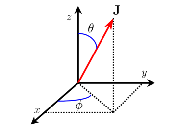
Figure 5.1: Angular momentum coordinates in the three-dimensional space.

As mentioned, the ground and first excited states have maximum angular momentum $j=1/2$. In Fig. 5.2 I show the orientation of the angular momentum in the ground states of the classical Hamiltonian $h_{c}$, represented by the vectors ${\bf J}$, ${\bf J_{1}}$, and ${\bf J_{2}}$, for different values of $V$ and $W$. When $\Delta=|V|-W\leq 1$ we have $\theta=\pi$ and the classical angular momentum is oriented in the negative $z$-direction. However, when $\Delta>1$ we have $\cos\theta=-\Delta^{-1}$ and the classical ground state becomes two-fold degenerate (notice that $h_{c}$ is invariant under the transformation $\phi\mapsto-\phi$). In this region and for $V<0$ the angular momentum is oriented in the XZ plane ($\phi=0$) while for $V>0$ it is oriented in the YZ plane ($\phi=\pm\pi/2$). The model has a gauge symmetry in the line $V=0$, $W<-1$, where $\phi$ can take any possible value.

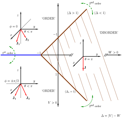
Figure 5.2: Representation of the classical ground state of the LMG model.

First and Second Order QPTs, and Critical Behavior

For the Hamiltonian of Eq. 5.1.1, the quantum system undergoes a second order QPT at the critical boundary $\Delta_{c}=|V_{c}|-W_{c}=1$, where for $\Delta>\Delta_{c}$ the ground and first excited states $|{g}\rangle$ and $|{e}\rangle$ become degenerate in the thermodynamic limit, and the inversion symmetry $K$ breaks. The order parameter is given by the mean number of fermions in the upper shell $\langle n_{\uparrow}\rangle=1/2+\langle J_{z}\rangle/N$, which in the thermodynamic limit converges to its classical value,

$$\lim_{N\rightarrow\infty}\langle n_{\uparrow}\rangle=\frac{1+\cos\theta}{2}\;.$$ (5.13)

Obviously, for $\Delta\leq\Delta_{c}$ one has $\langle n_{\uparrow}\rangle=0$, and $\langle n_{\uparrow}\rangle>0$, otherwise (Fig. 5.2). The critical exponents of the order parameter are easily computed by making a Taylor expansion near the critical points ($\Delta\rightarrow 1^{+}$). Defining the quantities $x=V_{c}-V$ and $y=W_{c}-W$, one obtains

$$\lim_{\Delta\rightarrow 1^{+}}\langle n_{\uparrow}\rangle=\left\{\begin{array}[]{l}(y^{\alpha}-x^{\beta})/2\hskip 8.53581pt\mbox{ for }V>0\\ (y^{\alpha}+x^{\beta})/2\hskip 8.53581pt\mbox{ for }V<0\end{array}\right.,$$

where the critical exponents are $\alpha=1$ and $\beta=1$.

In Fig. 5.3 I show the exact ground state energy per particle $E_{g}/N$ (with $E_{g}=\langle g|H|g\rangle$) as a function of $V$ and $W$ in the thermodynamic limit (Eqs. 5.11). One can see that also in the broken symmetry region ($\Delta>1$) the system undergoes a first order QPT at $V=0$; that is, the first derivative of the ground state energy with respect to $V$ is not continuous in this line.

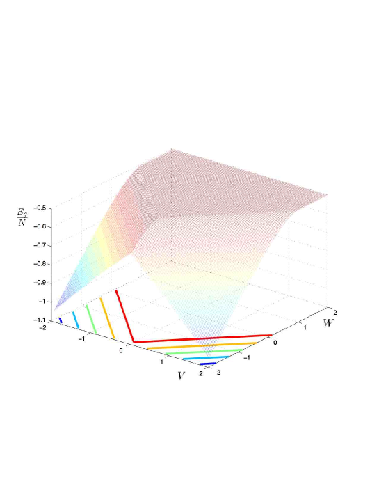
Figure 5.3: Ground state energy per particle in the LMG model.

Purity as an Indicator of the QPTs in the LMG Model

The standard notion of entanglement is not directly applicable to the LMG model as described by Eq. 5.8, as this is a single spin system and no physically natural partition into subsystems is possible. Therefore, using the $\mathfrak{h}$-purity as a measure of entanglement becomes an advantage from this point of view, since the latter only depends on a particular subset of observables and no partition of the system is necessary. The first required step is the identification of a relevant Lie algebra of observables relative to which the purity has to be calculated.

Since both the ground and first excited states of the quantum LMG model may be understood as states of a system carrying total angular momentum $J=N/2$, a first possible algebra to consider is the $\mathfrak{su}(N+1)$ algebra acting on the relevant $(N+1)$-dimensional eigenspace. Relative to this algebra, $|g\rangle$ is generalized unentangled for arbitrary values of $V$ and $W$, thus the corresponding purity remains constant and does not signal the QPTs. However, the family of Hamiltonians of Eq. 5.8 do not generate this Lie algebra, but rather an $\mathfrak{su}(2)$ algebra.

Thus a natural choice, suggested by the commutation relationships of Eqs. 5.6 and 5.7, is to study the purity relative to the spin-$N/2$ representation of the angular momentum Lie algebra $\mathfrak{h}=\mathfrak{su}(2)=\{J_{x},J_{y},J_{z}\}$:

$$P_{\mathfrak{h}}(|{\psi}\rangle)=\frac{4}{N^{2}}\Big{[}\langle J_{x}\rangle^{2}+\langle J_{y}\rangle^{2}+\langle J_{z}\rangle^{2}\Big{]}\;,$$ (5.14)

where the normalization factor ${\sf K}=N^{2}/4$ is chosen to ensure that the maximum of $P_{\mathfrak{h}}$ is equal to 1 (Eq. 3.32). With this normalization factor, $P_{\mathfrak{h}}$ can be calculated exactly in the thermodynamic limit by relying on the semi-classical approach described earlier (Appendix G and Eq. 5.9). For $V=0$ and arbitrary $W>0$, $|g\rangle=|J_{z}=-N/2\rangle$ which is a GCS of $\mathfrak{su}(2)$ and has $P_{\mathfrak{h}}=1$. For generic interaction values such that $\Delta\leq 1$, the classical angular momentum depicted in Fig. 5.2 is oriented along the $z$ direction and is not degenerate: Because $\langle J_{x}\rangle=\langle J_{y}\rangle=0$, only $\langle J_{z}\rangle$ contributes to $P_{\mathfrak{h}}$. By recalling that $\lim_{N\rightarrow\infty}\langle J_{z}/N\rangle=-1/2$, this gives $P_{\mathfrak{h}}=1$, so that as far as relative purity is concerned the ground state behaves asymptotically like a coherent state in the thermodynamic limit. Physically, this means that with respect to the relevant fluctuations, GCSs of $\mathfrak{su}(2)$ are a good approximation of the quantum ground state for large particle numbers, as is well established for this model [GF78]. However, in the region $\Delta>1$ the ground state (both classical and quantum) is two-fold degenerate in the $N\rightarrow\infty$ limit, and the value of $P_{\mathfrak{h}}$ depends in general on the particular linear combination of degenerate states. This can be understood from Fig. 5.2, where different linear combinations of the two degenerate vectors ${\bf J_{1}}$ and ${\bf J_{2}}$ imply different values of $\langle J_{x}\rangle$ for $V<0$ and different values of $\langle J_{y}\rangle$ for $V>0$, while $\langle J_{z}\rangle$ remains constant. With these features, the purity relative to the $\mathfrak{su}(2)$ algebra will not be a good indicator of the QPT.

An alternative option is then to look at a subalgebra of $\mathfrak{su}(2)$. In particular, if I only consider the purity relative to the single observable $\mathfrak{h}=\mathfrak{so}(2)=\{J_{z}\}$ (i.e., a particular CSA of $\mathfrak{su}(2)$), and retain the same normalization as above, then

$$P_{\mathfrak{h}}(|{\psi}\rangle)=\frac{4}{N^{2}}\langle J_{z}\rangle^{2}\;.$$ (5.15)

This new purity will be a good indicator of the QPT, since $P_{\mathfrak{h}}=1$ only for $\Delta\leq 1$ in the thermodynamic limit, and in addition $P_{\mathfrak{h}}$ does not depend on the particular linear combination of the two-fold degenerate states in the region $\Delta>1$, where $P_{\mathfrak{h}}<1$. Obviously, in this case $P_{\mathfrak{h}}$ is straightforwardly related to the order parameter (Eq. 5.13); the critical exponents of $P_{\mathfrak{h}}-1$ are indeed the same ($\alpha=1$ and $\beta=1$).

In the region $\Delta<1$ where $P_{\mathfrak{h}}=1$, the quantum ground state of the LMG model (Eq. 5.8) does not have a well defined $z$-component of angular momentum except at $V=0$ ($[H,J_{z}]\neq 0$ if $V\neq 0$), thus in general it does not lie on a coherent orbit of this algebra for finite $N$. However, as discussed above, it behaves asymptotically (in the infinite $N$ limit) as a GCS (in the sense that $P_{\mathfrak{h}}\rightarrow 1$).

In Fig. 5.4 I show the behavior of $P_{\mathfrak{h}}$ as a function of the parameters $V$ and $W$. The purity relative to $J_{z}$ is then a good indicator not only of the second order QPT but also of the first order QPT (the line $V=0$, $W<-1$).

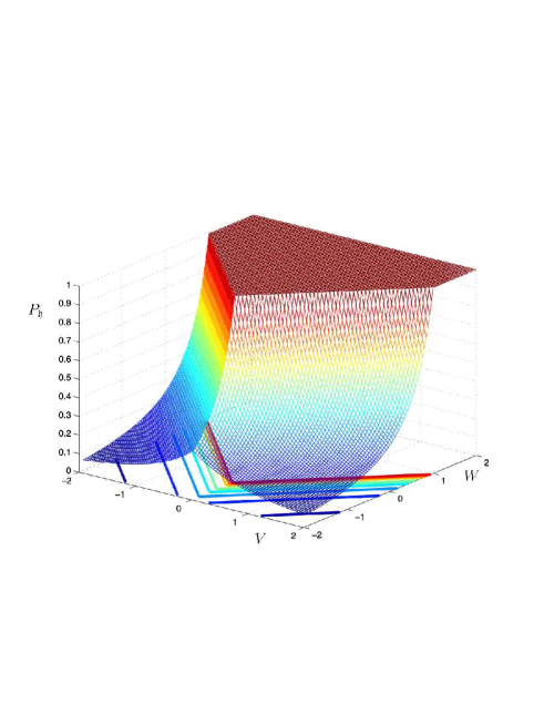
Figure 5.4: Purity relative to the observable $J_{z}$ in the ground state of the LMG model.

5.1.2 Anisotropic XY Model in a Transverse Magnetic Field

In this section, I exploit the purity relative to the $\mathfrak{u}(N)$ algebra (introduced in Sec. 3.3.3) as a measure of GE which is able to identify the paramagnetic-to-ferromagnetic QPT in the anisotropic one-dimensional spin-1/2 XY model in a transverse magnetic field and classify its universality properties.

The model Hamiltonian for a chain of $N$ sites is given by (Fig. 5.5)

$$H=-g\sum\limits_{i=1}^{N}\Big{[}(1+\gamma)\sigma_{x}^{i}\sigma_{x}^{i+1}+(1-\gamma)\sigma_{y}^{i}\sigma_{y}^{i+1}\Big{]}+\sum\limits_{i=1}^{N}\sigma_{z}^{i}\;,$$ (5.16)

where the operators $\sigma_{\alpha}^{i}$ ($\alpha=x,y,z$) are the Pauli spin-1/2 operators on site $i$ (Sec. 2.1), $g$ is the parameter one may tune to drive the QPT, and $0<\gamma\leq 1$ is the amount of anisotropy in the XY plane. In particular, for $\gamma=1$, Eq. 5.16 reduces to the Ising model in a transverse magnetic field [Pfe70], while for $\gamma\rightarrow 0$ the model becomes isotropic. Periodic boundary conditions are considered here, that is $\sigma_{\alpha}^{i+N}=\sigma_{\alpha}^{i}$, for all $i$ and $\alpha$.

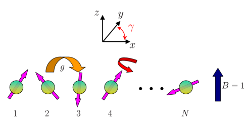
Figure 5.5: Anisotropic one-dimensional XY model in an external transverse magnetic field $B$.

When $g\gg 1$ and $\gamma=1$ the model is Ising-like. In this limit, the spin-spin interactions are the dominant contribution to the Hamiltonian (Eq. 5.16), and the ground state becomes degenerate in the thermodynamic limit, exhibiting ferromagnetic long-range order correlations in the $x$ direction: $M_{x}^{2}=\lim_{N\rightarrow\infty}\langle\sigma_{x}^{1}\sigma_{x}^{N/2}\rangle>0$, where $M_{x}$ is the magnetization in the $x$ direction. In the opposite limit where $g\rightarrow 0$, the external magnetic field becomes important, the spins tend to align in the $z$ direction, and the magnetization in the $x$ direction vanishes: $M_{x}^{2}=\lim_{N\rightarrow\infty}\langle\sigma_{x}^{1}\sigma_{x}^{N/2}\rangle=0$. Thus, in the thermodynamic limit the model is subject to a paramagnetic-to-ferromagnetic second order QPT at a critical point $g_{c}$ that will be determined later, with critical behavior belonging to the two-dimensional Ising model universality class.

This model can be exactly solved using the Jordan-Wigner transformation [JW28], which maps the Pauli (spin 1/2) algebra into the canonical fermion algebra through (Sec. 2.3.1)

$$c^{\dagger}_{j}=\prod\limits_{l=1}^{j-1}(-\sigma_{z}^{l})\sigma_{+}^{j}\;.$$ (5.17)

In order to find the exact ground state, I first need to write the Hamiltonian given in Eq. 5.16 in terms of these fermionic operators,

$$H=-2g\sum\limits_{i=1}^{N-1}(c^{\dagger}_{i}c^{\;}_{i+1}+\gamma c^{\dagger}_{i}c^{\dagger}_{i+1}+h.c.)+2gK(c^{\dagger}_{N}c^{\;}_{1}+\gamma c^{\dagger}_{N}c^{\dagger}_{1}+h.c.)+2\hat{N}\;,$$ (5.18)

where $K=\prod\limits_{j=1}^{N}(-\sigma_{z}^{j})$ is an operator that commutes with the Hamiltonian, and $\hat{N}=\sum\limits_{i=1}^{N}c^{\dagger}_{i}c^{\;}_{i}$ is the total number operator (here, I choose $N$ to be even). Then, the eigenvalue of $K$ is a good quantum number, and noticing that $K=e^{i\pi\hat{N}}$, one obtains $K=+1(-1)$ whenever the (non-degenerate) eigenstate of $H$ is a linear combination of states with an even (odd) number of fermions. In particular, the numerical solution of this model in finite systems (with $N$ even) indicates that the ground state has eigenvalue $K=+1$, implying anti-periodic boundary conditions in Eq. 5.18.

The second step is to rewrite the Hamiltonian in terms of the fermionic operators $\tilde{c}^{\dagger}_{k}$ ($\tilde{c}^{\;}_{k}$), defined by the Fourier transform of the operators $c^{\dagger}_{j}$ ($c^{\;}_{j}$):

$$\tilde{c}^{\dagger}_{k}=\frac{1}{\sqrt{N}}\sum\limits_{j=1}^{N}e^{-ikj}c^{\dagger}_{j}\;,$$ (5.19)

where the set $V$ of possible $k$ is determined by the anti-periodic boundary conditions in the fermionic operators: $V=V_{+}+V_{-}=[\pm\frac{\pi}{N},\pm\frac{3\pi}{N},\cdots,\pm\frac{(N-1)\pi}{N}]$. Therefore,

$$H+N=-2\sum\limits_{k\epsilon V}(-1+2g\cos k)\tilde{c}^{\dagger}_{k}\tilde{c}^{\;}_{k}+ig\gamma\sin k(\tilde{c}^{\dagger}_{-k}\tilde{c}^{\dagger}_{k}+\tilde{c}^{\;}_{-k}\tilde{c}^{\;}_{k})\;.$$ (5.20)

The third and final step is to diagonalize the Hamiltonian of Eq. 5.20 using the Bogolubov canonical transformation [BR86]

$$\left\{\begin{array}[]{l}\gamma_{k}=u_{k}\tilde{c}^{\;}_{k}-iv_{k}\tilde{c}^{\dagger}_{-k}\\ \gamma^{\dagger}_{-k}=u_{k}\tilde{c}^{\dagger}_{-k}-iv_{k}\tilde{c}^{\;}_{k}\end{array}\right.\;,$$

where the real coefficients $u_{k}$ and $v_{k}$ satisfy the relations

$$u_{k}=u_{-k}\mbox{, }v_{k}=-v_{-k}\;,\mbox{ and }\;u_{k}^{2}+v_{k}^{2}=1\;,$$ (5.21)

with

$$u_{k}=\cos\Big{(}\frac{\phi_{k}}{2}\Big{)}\;,\mbox{ }v_{k}=\sin\Big{(}\frac{\phi_{k}}{2}\Big{)}\;,$$ (5.22)

and $\phi_{k}$ given by

$$\tan(\phi_{k})=\frac{2g\gamma\sin k}{-1+2g\cos k}\;.$$ (5.23)

In this way, the quasiparticle creation and annihilation operators $\gamma^{\dagger}_{k}$ and $\gamma^{\;}_{k}$, also satisfy the canonical fermionic anti-commutation relations of Eq. 2.34, and the Hamiltonian may be finally rewritten as

$$H=\sum\limits_{k\epsilon V}\xi_{k}(\gamma^{\dagger}_{k}\gamma^{\;}_{k}-1/2)\;,$$ (5.24)

where $\xi_{k}=2\sqrt{(-1+2g\cos k)^{2}+4g^{2}\gamma^{2}\sin^{2}k}$ is the quasiparticle energy. Since in general $\xi_{k}>0$, the ground state is the quantum state with no quasiparticles (BCS state [Tak99]), such that $\gamma_{k}|{\sf BCS}\rangle=0$. Thus, one finds

$$|{\sf BCS}\rangle=\prod\limits_{k\epsilon V_{+}}(u_{k}+iv_{k}\tilde{c}^{\dagger}_{k}\tilde{c}^{\dagger}_{-k})|{\sf vac}\rangle\;,$$ (5.25)

where $|{\sf vac}\rangle$ is the state with no fermions ($\tilde{c}_{k}|{\sf vac}\rangle=0$).

Excited states with an even number of fermions ($K=+1$) can be obtained applying pairs of quasiparticle creation operators $\gamma^{\dagger}_{k}$ to the $|{{\sf BCS}}\rangle$ state. However, one should be more rigorous when obtaining excited states with an odd number of particles, since $K=-1$ implies periodic boundary conditions in Eq. 5.18, and the new set of possible $k$’s (wave vectors) is $\overline{V}=[-\pi,\cdots,-\frac{2\pi}{N},0,\frac{2\pi}{N},\cdots,\frac{2(N-1)\pi}{N}]$ (different from $V$).

QPT and Critical Point

In Fig. 5.6 I show the order parameter $M_{x}^{2}=\lim_{N\rightarrow\infty}\langle\sigma_{x}^{1}\sigma_{x}^{N/2}\rangle$ as a function of $g$ in the thermodynamic limit and for different anisotropies $\gamma$ [BM71]. Then, $M_{x}^{2}=0$ for $g\leq g_{c}$ and $M_{x}^{2}\neq 0$ for $g>g_{c}$, so the critical point is located at $g_{c}=1/2$, regardless of the value of $\gamma$. The value of $g_{c}$ can also be obtained by setting $\xi_{k}=0$ in Eq. 5.24, where the gap vanishes.

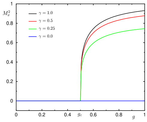
Figure 5.6: Order parameter $M_{x}^{2}$ in the thermodynamic limit as a function of $g$ for different anisotropies $\gamma$. The critical point is at $g_{c}=1/2$.

The Hamiltonian of Eq. 5.16 is invariant under the transformation that maps $(\sigma_{x}^{i};\sigma_{y}^{j};\sigma_{z}^{k})\mapsto(-\sigma_{x}^{i};-\sigma_{y}^{j};\sigma_{z}^{k})$ ($\mathbb{Z}_{2}$ symmetry), implying that $\langle\sigma_{x}^{i}\rangle=0$ for all $g$. However, since in the thermodynamic limit the ground state becomes two-fold degenerate, for $g>g_{c}$ , it is possible to build up a ground state where the discrete $\mathbb{Z}_{2}$ symmetry is broken, i.e. $\langle\sigma_{x}^{i}\rangle\neq 0$. This statement can be easily understood if we consider the case of $\gamma=1$, where for $0\leq g<g_{c}$ the ground state has no magnetization in the $x$ direction: For $g=0$, the spins align with the magnetic field, while an infinitesimal spin interaction disorders the system and $M_{x}=0$. On the other hand, for $g\rightarrow\infty$ the states $|{g_{1}}\rangle=\frac{1}{\sqrt{2}}[|{\rightarrow,\cdots,\rightarrow}\rangle+|{\leftarrow,\cdots,\leftarrow}\rangle]$ and $|{g_{2}}\rangle=\frac{1}{\sqrt{2}}[|{\rightarrow,\cdots,\rightarrow}\rangle-|{\leftarrow,\cdots,\leftarrow}\rangle],$ with $|{\rightarrow}\rangle=\frac{1}{\sqrt{2}}[|{\uparrow}\rangle+|{\downarrow}\rangle]$ and $|{\leftarrow}\rangle=\frac{1}{\sqrt{2}}[|{\uparrow}\rangle-|{\downarrow}\rangle]$, become degenerate in the thermodynamic limit, and a ground state with $\langle\sigma_{x}^{i}\rangle\neq 0$ can be constructed from a linear combination.

Remarkably, this paramagnetic-to-ferromagnetic QPT does not exist in the isotropic limit ($\gamma=0$). In this case, the Hamiltonian of Eq. 5.16 has a continuous $\mathfrak{u}(1)$ symmetry; that is, it is invariant under any $\hat{z}$ rotation of the form $\exp[i\theta\sum_{j}\sigma_{z}^{j}]$. Since the model is one-dimensional, this symmetry cannot be spontaneously broken, regardless of the magnitude of the coupling constants. Nevertheless, a simple calculation of the ground state energy indicates a divergence in its second derivative at the critical point $g_{c}=1/2$, thus, a second order non-broken symmetry QPT. For $g<g_{c}$ all the spins (in the ground state) are aligned with the external magnetic field, with total magnetization in the $\hat{z}$ direction $M_{z}=\sum_{j}\langle\sigma_{z}^{j}\rangle=-N$, and the quantum phase is gapped. For $g\geq g_{c}$, the total magnetization in the $\hat{z}$ direction is $M_{z}\geq-N$, the gap vanishes, and the quantum phase becomes critical (i.e., the spin-spin correlation functions decay with a power law), with an emergent $\mathfrak{u}(1)$ gauge symmetry [BO04]. Then, in terms of fermionic operators (Eq. 5.18), an insulator-metal (or superfluid) like second order QPT exists at $g_{c}$ for the isotropic case, with no symmetry order parameter. It is a Lifshitz transition.

$\mathfrak{u}(N)$-Purity in the BCS State and Critical Behavior

The $|{\sf BCS}\rangle$ state of Eq. 5.25 is a GCS of the algebra of observables $\mathfrak{h}=\mathfrak{so}(2N)$. This is spanned by an orthonormal Hermitian basis which is constructed by adjoining to the basis of $\mathfrak{u}(N)$, given in Eq. 3.53, the following set $\mathfrak{r}$ of number-non-conserving fermionic operators:

$$\mathfrak{r}=\left\{\begin{array}[]{ll}(c^{\dagger}_{j}c^{\dagger}_{j^{\prime}}+c^{\;}_{j^{\prime}}c^{\;}_{j})&\mbox{ with }1\leq j<j^{\prime}\leq N\cr i(c^{\dagger}_{j}c^{\dagger}_{j^{\prime}}-c^{\;}_{j^{\prime}}c^{\;}_{j})&\mbox{ with }1\leq j<j^{\prime}\leq N\cr\end{array}\right.\>,\hskip 14.22636pt\mathfrak{so}(2N)=\mathfrak{u}(N)\oplus\mathfrak{r}\>.$$ (5.26)

Then, the $|{\sf BCS}\rangle$ state is generalized unentangled with respect to the $\mathfrak{so}(2N)$ algebra and its purity $P_{\mathfrak{h}}$ contains no information about the phase transition: $P_{\mathfrak{h}}=1\mbox{ }\forall g,\gamma$. Therefore, in order to characterize the QPT one needs to look at the possible subalgebras of $\mathfrak{so}(2N)$. A natural choice is to restrict to operators which preserve the total fermion number, that is, to consider the $\mathfrak{u}(N)$ algebra defined in Sec. 3.3.3, relative to which the $|{\sf BCS}\rangle$ state may become generalized entangled. (Note that as mentioned in Sec. 3.3.3, the $\mathfrak{u}(N)$ algebra can also be written in terms of the fermionic operators $\tilde{c}^{\dagger}_{k}$ and $\tilde{c}_{k}$, with $k$ belonging to the set $V$.)

In the $|{\sf BCS}\rangle$ state, $\langle\tilde{c}^{\dagger}_{k}\tilde{c}^{\;}_{k^{\prime}}\rangle\neq 0$ only if $k=k^{\prime}$, thus using Eq. 3.54 the purity relative to $\mathfrak{h}=\mathfrak{u}(N)$ is:

$$P_{\mathfrak{h}}(|{\sf BCS}\rangle)=\frac{4}{N}\sum\limits_{k\epsilon V}\langle\tilde{c}^{\dagger}_{k}\tilde{c}^{\;}_{k}-1/2\rangle^{2}=\frac{4}{N}\sum\limits_{k\epsilon V}(v_{k}^{2}-1/2)^{2}\;,$$ (5.27)

where the coefficients $v_{k}$ can be obtained from Eqs. 5.22 and 5.23. In particular, for $g=0$ the spins are aligned with the magnetic field and the fully polarized $|{\sf BCS}\rangle_{g=0}=|{\downarrow,\downarrow,\ldots,\downarrow}\rangle$ state is generalized unentangled in this limit (a GCS of $\mathfrak{u}(N)$ with $P_{\mathfrak{h}}=1$). In the thermodynamic limit, the purity relative to the $\mathfrak{u}(N)$ algebra can be obtained by integrating Eq. 5.27:

$$P_{\mathfrak{h}}(|{\sf BCS}\rangle)=\frac{2}{\pi}\int\limits_{0}^{2\pi}(v_{k}^{2}-1/2)^{2}dk\>,$$ (5.28)

leading to the following result:

$$P_{\mathfrak{h}}(|{\sf BCS}\rangle)=\left\{\begin{array}[]{cl}\frac{1}{1-\gamma^{2}}\Big{[}1-\frac{\gamma^{2}}{\sqrt{1-4g^{2}(1-\gamma^{2})}}\Big{]}&\mbox{ if }g\leq 1/2\\ \frac{1}{1+\gamma}&\mbox{ if }g>1/2\end{array}\right.\;.$$ (5.29)

Although this function is continuous, its derivative is not and has a drastic change at $g=1/2$, where the QPT occurs. Moreover, $P_{\mathfrak{h}}$ is minimum for $g>1/2$ implying maximum entanglement at the transition point and in the ordered (ferromagnetic) phase. Remarkably, for $g>1/2$ and $N\rightarrow\infty$, where the ground state of the anisotropic XY model in a transverse magnetic field is two-fold degenerate, $P_{\mathfrak{h}}$ remains invariant for arbitrary linear combinations of the two degenerate states.

As defined, for large $g$ the purity $P_{\mathfrak{h}}$ approaches a constant value which depends on $\gamma$. It is convenient to remove such dependence in the ordered phase by introducing a new quantity $P^{\prime}_{\mathfrak{h}}=P_{\mathfrak{h}}-\frac{1}{1+\gamma}$ (shifted purity). Thus,

$$P^{\prime}_{\mathfrak{h}}(|{\sf BCS}\rangle)=\left\{\begin{array}[]{cl}\frac{\gamma}{1-\gamma^{2}}\Big{[}1-\frac{\gamma}{\sqrt{1-4g^{2}(1-\gamma^{2})}}\Big{]}&\mbox{ if }g\leq 1/2\\ 0&\mbox{ if }g>1/2\end{array}\right.\;.$$ (5.30)

The new function $P^{\prime}_{\mathfrak{h}}$ behaves like a disorder parameter for the system, being zero in the ferromagnetic (ordered) phase and different from zero in the paramagnetic (disordered) one. The behavior of $P^{\prime}_{\mathfrak{h}}$ as a function of $g$ in the thermodynamic limit is depicted in Fig. 5.7 for different values of $\gamma$. In the special case of the Ising model in a transverse magnetic field ($\gamma=1$), one has the simple behavior $P^{\prime}_{\mathfrak{h}}=1/2-2g^{2}$ for $g\leq 1/2$ and $P^{\prime}_{\mathfrak{h}}=0$ if $g>1/2$.

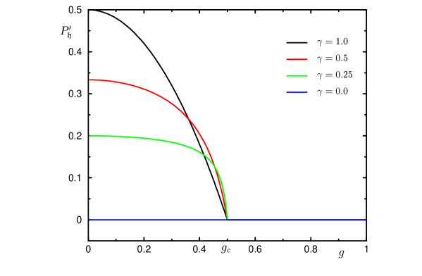
Figure 5.7: Shifted purity $P^{\prime}_{\mathfrak{u}(N)}$ of the $|{\sf BCS}\rangle$ as a function of $g$ for different anisotropies $\gamma$, Eq. 5.30. $P^{\prime}_{\mathfrak{u}(N)}$ behaves like a disorder parameter for this model, sharply identifying the QPT at $g_{c}=1/2$.

The critical behavior of the system is characterized by a power-law divergence of the correlation length $\epsilon$, which is defined such that for $g<1/2$,

$$\lim_{|i-j|\rightarrow\infty}|\langle\sigma_{x}^{i}\sigma_{x}^{j}\rangle|\sim\exp(-\frac{|i-j|}{\epsilon}).$$ (5.31)

Thus, $\epsilon\rightarrow\infty$ signals the emergence of long-range correlations in the ordered region $g>1/2$. Near the critical point ($g\rightarrow 1/2^{-}$), the correlation length behaves as $\epsilon\sim(g_{c}-g)^{-\nu}$, where $\nu$ is a critical exponent and the value $\nu=1$ corresponds to the Ising universality class. Let the parameter $\lambda_{2}=e^{-1/\epsilon}$. The fact that the purity contains information about the critical properties of the model follows from the possibility of expressing $P^{\prime}_{\mathfrak{h}}$ for $g<1/2$ as a function of the correlation length,

$$P^{\prime}_{\mathfrak{h}}(|{\sf BCS}\rangle)=\frac{\gamma}{1-\gamma^{2}}\left[1+\frac{\gamma}{2g\lambda_{2}(1-\gamma)-1}\right]\ ,$$ (5.32)

where a known relation between $g$, $\gamma$, and $\lambda_{2}$ has been exploited [BM71]. Performing a Taylor expansion of Eq. 5.32 in the region $g\rightarrow 1/2^{-}$, one obtains (Fig. 5.8)

$$P^{\prime}_{\mathfrak{h}}\sim 2(g_{c}-g)^{\nu}/\gamma\ \ \nu=1,\gamma>0.$$ (5.33)

Thus, the name disorder parameter for $P^{\prime}_{\mathfrak{h}}$ is consistent.

Figure 5.8: Scaling properties of the disorder parameter for anisotropy $\gamma=1$. The exponent $\nu=1$ belongs to the Ising universality class.

Some physical insight into the meaning of the ground-state purity may be gained by noting that Eq. 5.27 can be written in terms of the fluctuations of the total fermion operator $\hat{N}$

$$P_{\mathfrak{h}}(|{\sf BCS}\rangle)=1-\frac{2}{N}\Big{(}\langle\hat{N}^{2}\rangle-\langle\hat{N}\rangle^{2}\Big{)}\;,$$ (5.34)

where the $|{\sf BCS}\rangle$-property $\langle\tilde{c}^{\dagger}_{k}\tilde{c}_{k^{\prime}}\rangle=\delta_{k,k^{\prime}}v_{k}^{2}$ has been used. In general, the purity relative to a given algebra can be written in terms of fluctuations of observables [BKO03].

Since fluctuations of observables are at the root of QPTs, it is not surprising that this quantity succeeds at identifying the critical point. Interestingly, by recalling that $P_{\mathfrak{so}(2N)}(|{\sf BCS}\rangle)=1$, the $\mathfrak{u}(N)$-purity can also be formally expressed as

$$P_{\mathfrak{u}(N)}(|{\sf BCS}\rangle)=1-\sum_{A_{\alpha}\in\mathfrak{r}}\langle A_{\alpha}\rangle^{2}\>,$$ (5.35)

where the sum only extends to the non-number-conserving $\mathfrak{so}(2N)$-generators belonging to the set $\mathfrak{r}$ specified in Eq. 5.26. Thus, the purity is entirely contributed by expectations of operators connecting different $\mathfrak{u}(N)$-irreps, the net effect of correlating representations with a different particle number resulting in the fluctuation of a single operator, given by $\hat{N}=\sum_{k}\tilde{c}_{k}^{\dagger}\tilde{c}_{k}$. In Fig. 5.9, I show the probability $\Omega(n)$ of having $n$ fermions in a chain of $N=400$ sites for $\gamma=1$. For $g>1/2$ the fluctuations remain almost constant, and so does the purity.

Figure 5.9: Distribution of the fermion number in the $|{\sf BCS}\rangle$ state for a chain of $N=400$ sites and anisotropy $\gamma=1$.

Again, the isotropic case ($\gamma=0$) is particular in the sense that $P_{\mathfrak{h}}=1$ (or $P^{\prime}_{\mathfrak{h}}=0$, see Fig. 5.7), without identifying the corresponding metal-insulator QPT. The reason is that in this limit, the Hamiltonian of Eq. 5.18 contains only fermionic operators that preserve the number of particles (i.e., $H\in\mathfrak{u}(N)$), and the ground state of the system is always a GCS of the $\mathfrak{u}(N)$ algebra. Therefore, in order to obtain information about this QPT, one should look at algebras other than $\mathfrak{u}(N)$, relative to which the ground state is generalized entangled. A more detailed analysis can be found in Ref. [SOB04].

5.2 General Mean-Field Hamiltonians

A Lie-algebraic analysis of many-body problems leads to a powerful tool for finding the spectrum and eigenstates of the Hamiltonian that describes the interactions in the system:

$$H=\sum_{j=1}^{M}\kappa_{j}\hat{O}_{j},\ \kappa_{j}\in\mathbb{R},$$ (5.36)

where the Hermitian operators $\hat{O}_{j}$ are linearly independent Schmidt-orthogonal elements of a Lie algebra $\mathfrak{h}=\{\hat{O}_{1},\cdots\hat{O}_{M}\}$ (Sec. 3.2.2). Each operator $\hat{O}_{j}$ corresponds to a $d\times d$ matrix acting on the Hilbert space $\cal H$ (of dimension $d$) associated with the physical system. In general, $d$ is infinite or scales exponentially with a certain variable $N$, like the volume of the system, etc. For example, for a $N$-spin-1/2 system one obtains $d=2^{N}$. However, if the system is bosonic or is composed of harmonic oscillators, then $d\rightarrow\infty$. Throughout this section, I will assume that $N\leq\mbox{poly}[\log(d)]$.

Without loss of generality, one can consider $\mathfrak{h}$ to be a semi-simple Lie algebra acting irreducibly on $\cal H$: The Casimir elements in $H$ behave as constants (symmetries) and do not change the physics. If the dimension of $\mathfrak{h}$ satisfies $M\leq\mbox{poly}(N)$, then $H$ is defined to be a general mean field Hamiltonian and is denoted as $H_{MF}$. Since $\mathfrak{h}$ admits a CW decomposition (see Sec. 3.2.2), one obtains

$$H_{MF}=\sum\limits_{k=1}^{r}\gamma_{k}\hat{h}_{k}+\sum\limits_{j=1}^{l}\iota_{j}\hat{E}_{\alpha_{j}}+\iota^{*}_{j}\hat{E}_{-\alpha_{j}},$$ (5.37)

where $\gamma_{k}\in\mathbb{R}$ and $\iota_{j}\in\mathbb{C}$ are known (or can easily be computed) coefficients, $\hat{h}_{k}\in\mathfrak{h}_{D}$ (i.e., the CSA of $\mathfrak{h}$), $\hat{E}_{\pm\alpha_{j}}$ are ladder operators, and $(r,l)\leq\mbox{poly}(N)$.

The eigenstates $|{\phi^{p}}\rangle$ of $\mathfrak{h}_{D}$ (i.e., the weight states of the standard representation given by $\cal H$) and the corresponding eigenvalues $e_{k}^{p}$, satisfying

$$\hat{h}_{k}|{\phi^{p}}\rangle=e_{k}^{p}|{\phi^{p}}\rangle,$$ (5.38)

are assumed to be known with high accuracy. In particular, every weight state can always be obtained by the (efficient) successive application of lowering operators to a highest weight state $|{{\sf HW}}\rangle\in\cal H$:

$$|{\phi^{p}}\rangle=N_{p}\prod\limits_{j=1}^{l}\hat{E}_{-\alpha_{j}}^{n_{j}}|{\sf HW}\rangle,$$ (5.39)

where $N_{p}\in\mathbb{R}$ is a normalization factor ($n_{j}\in\mathbb{Z}$). If $(e_{1},\cdots,e_{r})$ is the highest weight vector (associated with $|{\sf HW}\rangle$), then

$$\hat{h}_{k}|{\phi^{p}}\rangle=\left[e_{k}-\sum\limits_{j=1}^{l}n_{j}\alpha_{j}^{k}\right]|{\phi^{p}}\rangle.$$ (5.40)

Therefore, all the information about the weight states of $\mathfrak{h}$ can be obtained from $|{\sf HW}\rangle$, its weights, and the root vectors $\alpha_{j}$. This applies to every irreducible representation of $\mathfrak{h}$.

The diagonal form $H_{D}\in\mathfrak{h}_{D}$ of Eq. 5.37 is the Hermitian operator

$$H_{D}=\sum\limits_{k=1}^{r}\varepsilon_{k}\hat{h}_{k}=UHU^{\dagger},$$ (5.41)

where $U=e^{iF}$ is a unitary operator ($F=F^{\dagger}$). In principle, $U$ and $H_{D}$ can be obtained by a simple matrix diagonalization algorithm working in some low-dimensional faithful representation of $\mathfrak{h}$. However, this is not sufficient to show that the eigenvectors and eigenvalues obtained correspond to a group operation and an element in $\mathfrak{h}_{D}$, respectively. Nevertheless, an important result in Lie theory states that an operator such as $U$ can always be chosen to be a group operator induced by $\mathfrak{h}$, that is

$$F=\sum\limits_{j=1}^{M}\zeta_{j}\hat{O}_{j}\ ,\in\mathfrak{h}.$$ (5.42)

Because $H_{D}\in\mathfrak{h}_{D}$, its eigenstates are the weight states $|{\phi^{p}}\rangle$ of Eq. 5.39. Then,

$$|{\tilde{\phi}^{p}}\rangle=U^{\dagger}|{\phi^{p}}\rangle=N_{p}U^{\dagger}\prod_{j=1}^{l}\hat{E}^{n_{j}}_{-\alpha_{j}}|{\sf HW}\rangle$$ (5.43)

are the eigenstates of $H$. In particular, $F$ can be chosen such that $|{{\sf HW}}\rangle$ is the ground state of Eq. 5.41 and

$$|{G}\rangle=U^{\dagger}|{\sf HW}\rangle$$ (5.44)

is the ground state of Eq. 5.37. Therefore, $|{G}\rangle$ is generalized unentangled and GCS of $\mathfrak{h}$. Moreover, considering that $U$ is a similarity transformation, the spectrum of Eq. 5.37 is then given by

$$H|{\tilde{\phi}^{p}}\rangle=\left[\sum\limits_{k=1}^{r}\varepsilon_{k}e_{k}^{p}\right]|{\tilde{\phi}^{p}}\rangle,$$ (5.45)

where the weights $e_{k}^{p}$ can be obtained from the highest weight vector as in Eq. 5.40.

In brief, Eq. 5.37 is diagonalized if the coefficients $\varepsilon_{k}$ of Eq. 5.41 and $\zeta_{j}$ of Eq. 5.42 are obtained. This can be done in any faithful representation of $\mathfrak{h}$. To show this, assume that $\bar{O}_{j}$ is any faithful matrix representation associated to the operator $\hat{O}_{j}$. From the definition of the exponential mapping, one obtains

$$e^{iF}He^{-iF}=H+i\left[F,H\right]-\frac{1}{2}\left[F,\left[F,H\right]\right]+\cdots=\sum\limits_{k=1}^{r}\varepsilon_{k}\hat{h}_{k},$$ (5.46)

and, equivalently,

$$e^{i\bar{F}}\bar{H}e^{-i\bar{F}}=\bar{H}+i\left[\bar{F},\bar{H}\right]-\frac{1}{2}\left[\bar{F},\left[\bar{F},\bar{H}\right]\right]+\cdots=\sum\limits_{k=1}^{r}\varepsilon_{k}\bar{h}_{k},$$ (5.47)

which is the matrix representation of Eq. 5.46. Since $M\leq\mbox{poly}(N)$, then $H_{MF}$ can be exactly diagonalized using the classical algorithm given in the following section.

5.2.1 Diagonalization Procedure

Any element $H$ of a real semi-simple Lie algebra $\mathfrak{h}$ can be diagonalized through a similarity group transformation induced by $\mathfrak{h}$. Based on Ref. [Wil93], in this section I introduce a classical algorithm for the diagonalization when $\mathfrak{h}$ is also a compact Lie algebra. This algorithm is a generalization of the well known Jacobi’s algorithm [PTV92] used for general matrix diagonalization.

Assume then that $\Phi$ is a faithful matrix representation of $\mathfrak{h}=\{\hat{O}_{1},\cdots,\hat{O}_{M}\}$, satisfying

$${\sf Tr}\left[\bar{O}_{j}\bar{O}_{j^{\prime}}\right]=\delta_{jj^{\prime}},$$ (5.48)

with $\bar{O}_{j}=\Phi(O_{j})$. Equation 5.48 is always satisfied in the case of compact Lie algebras if working with the adjoint representation. In general, an orthogonal basis is given by the Hermitian matrices $\bar{h}_{k}$, $[\bar{E}_{\alpha_{j}}+\bar{E}_{-\alpha_{j}}]$, and $i[\bar{E}_{\alpha_{j}}-\bar{E}_{-\alpha_{j}}]$ (up to normalization factors), which are representations of the operators in the CSA of $\mathfrak{h}$ and in the set of ladder operators, respectively. Therefore, the trace inner product of Eq. 5.48 allows one to project any operator in $\mathfrak{h}$ onto the sets $\mathfrak{h}_{D}$, $\mathfrak{h}_{+}$, and $\mathfrak{h}_{-}$. That is, the coefficients $\gamma_{k}$ and $\iota_{j}$ of Eq. 5.37 can be obtained by projecting the matrix $\bar{H}_{MF}$, associated to $H_{MF}$, onto the representations of the corresponding operators.

To find the group operation $U$ of Eq. 5.41, one starts by searching classically the index $t$ such that $|\iota_{t}|\geq|\iota_{j}|\ \forall j\in[1\cdots l]$. Second, one needs to perform a particular group (unitary) operation $U_{t}$ such that the transformed operator $H^{1}=U_{t}H^{0}U_{t}^{\dagger}$, with $H^{0}\equiv H_{MF}$, is

$$H^{1}=\sum\limits_{k=1}^{r}\gamma^{1}_{k}\hat{h}_{k}+\sum\limits_{j=1}^{l}\iota^{1}_{j}\hat{E}_{\alpha_{j}}+(\iota^{1}_{j})^{*}\hat{E}_{-\alpha_{j}}\ ;\ \iota^{1}_{t}=0.$$ (5.49)

The operator $U_{t}$ can be obtained by noticing the existence in $\mathfrak{h}$ of the $\mathfrak{su}^{t}(2)$ Lie algebra

$$\mathfrak{su}^{t}(2)\left\{\matrix{S_{+}^{t}&=&\left[\sum_{k}(\alpha^{k}_{t})^{2}\right]^{-1}\hat{E}_{\alpha_{t}},\cr S_{-}^{t}&=&\left[\sum_{k}(\alpha^{k}_{t})^{2}\right]^{-1}\hat{E}_{-\alpha_{t}},\cr S_{z}^{t}&=&\left[\sum_{k}(\alpha^{k}_{t})^{2}\right]^{-2}\left[\sum_{k}\alpha^{k}_{t}\hat{h}_{k}\right],}\right.$$ (5.50)

where $\alpha_{t}^{k}$ are the components of the associated root vector. The operators $S_{x}^{t}$ and $S_{y}^{t}$ are obtained from the relations $S_{\pm}^{t}=\frac{1}{2}[S_{x}^{t}\pm iS_{y}^{t}]$. Since $\hat{h}_{k}$, $\hat{E}_{\alpha_{j}}$, and $\hat{E}_{-\alpha_{j}}$ satisfy the commutation relations defined in Sec. 3.2.2, the operators $S_{x}^{t}$, $S_{y}^{t}$, and $S_{z}^{t}$ satisfy the $\mathfrak{su}(2)$ commutation relations of Eqs. 2.4 (i.e., spin operators). Equation 5.37 can then be written as

$$H=H_{t}+H_{t}^{\perp},$$ (5.51)

where $H_{t}=\nu^{t}_{x}S^{t}_{x}+\nu^{t}_{y}S^{t}_{y}+\nu^{t}_{z}S^{t}_{z}\in\mathfrak{su}^{t}(2),\ \nu^{t}_{\alpha}\in\mathbb{R}$, and $H_{t}^{\perp}$ is an element of the orthogonal complement $\mathfrak{su}^{t}(2)^{\perp}$ as defined by Eq. 5.48.

Therefore, $U_{t}$ is defined as the operator in the group $SU^{t}(2)\equiv e^{i\mathfrak{su}^{t}(2)}$ that diagonalizes $H_{t}\in\mathfrak{su}^{t}(2)$. That is,

$$U_{t}=\exp\left[i(\mu^{t}_{x}S^{t}_{x}+\mu^{t}_{y}S^{t}_{y}+\mu^{t}_{z}S^{t}_{z})\right],$$ (5.52)

where $\mu^{t}_{\alpha}\in\mathbb{R}$, and

$$U_{t}H_{t}U_{t}^{\dagger}\propto S_{z}^{t}\in\mathfrak{h}_{D}.$$ (5.53)

This is a diagonalization problem in $\mathfrak{su}(2)$ and the defining coefficients $\mu^{t}_{\alpha}$ of Eq. 5.52 can be obtained through the diagonalization of a $2\times 2$ matrix.

Remarkably, $U_{t}$ leaves invariant the decomposition

$$\mathfrak{h}=\mathfrak{su}^{t}(2)\oplus\mathfrak{h}_{D}^{t,\perp}\oplus\mathfrak{h}_{\pm}^{t,\perp},$$ (5.54)

where $\mathfrak{h}_{D}^{t,\perp}$ and $\mathfrak{h}_{\pm}^{t,\perp}$ are the sets of operators in $\mathfrak{h}_{D}$ and $(\mathfrak{h}_{+}\oplus\mathfrak{h}_{-})$, respectively, which are orthogonal to $\mathfrak{su}^{t}(2)$. To show this, I first notice that

$$\left[\mathfrak{su}^{t}(2),\mathfrak{h}_{D}^{t,\perp}\right]=0,$$ (5.55)

or otherwise a group operation in $SU^{t}(2)\equiv e^{i\mathfrak{su}^{t}(2)}$ could transform operators in $\mathfrak{h}_{D}^{t,\perp}$ into operators in $\mathfrak{su}^{t}(2)$. This is not allowed due to the orthogonalization property of Eq. 5.48. For the same reason,

$$\left[\mathfrak{su}^{t}(2),\mathfrak{h}_{\pm}^{t,\perp}\right]\subset\mathfrak{h}_{\pm}^{t,\perp}.$$ (5.56)

Equations 5.55 and 5.56 are sufficient to guarantee the invariance of the decomposition in Eq. 5.54 under the action of $U_{t}$. Then, such $U_{t}$ anihilates the $t$-component of $H_{MF}$ and transforms it as in Eq. 5.49.

The same $\mathfrak{su}(2)$-diagonalization procedure is applied to $H^{1}$ and so on, to obtain $H^{2},\cdots,H^{p}$. In each step, a certain component $t$ is eliminated as described above. Therefore, $H^{p}$ gets closer to a diagonal form and

$$\lim_{p\rightarrow\infty}H^{p}\subset\mathfrak{h}_{D}.$$ (5.57)

To show this, I first write $H^{p}$ as

$$H^{p}=\sum\limits_{k=1}^{r}\gamma^{p}_{k}\hat{h}_{k}+\sum\limits_{j=1}^{l}\iota^{p}_{j}\hat{E}_{\alpha_{j}}+(\iota^{p}_{j})^{*}\hat{E}_{-\alpha_{j}},$$ (5.58)

where $H^{0}\equiv H_{MF}$ and $\gamma^{0}_{k}=\gamma_{k}$, $\iota^{0}_{j}=\iota_{j}$. The square distance of $H^{p}$ to $\mathfrak{h}_{D}$ is defined as

$$d_{C}(H^{p})=\sum\limits_{j=1}^{l}|\iota^{p}_{j}|^{2},$$ (5.59)

which is equivalent to count for the off-diagonal elements as in the Jacobi’s diagonalization algorithm for symmetric matrices [PTV92]. In particular, $d_{C}(H^{p})=0$ when $H^{p}\in\mathfrak{h}_{D}$. If $t$ denotes the index of the biggest $|\iota^{p-1}_{j}|$ in the $p-1$ iteration, then

$$\sum\limits_{j=1}^{l}|\iota^{p-1}_{j}|^{2}\leq l|\iota^{p-1}_{t}|^{2}.$$ (5.60)

Moreover, since $U_{t}$ leaves $\mathfrak{h}_{\pm}^{t,\perp}$ invariant (Eq. 5.54), then

$$d_{C}(H^{p})=\sum\limits_{j=1(\neq t)}^{l}|\iota^{p}_{j}|^{2}=\sum\limits_{j=1(\neq t)}^{l}|\iota^{p-1}_{j}|^{2}.$$ (5.61)

Therefore,

$$d_{c}(H^{p})=\sum\limits_{j=1(\neq t)}^{l}|\iota^{p-1}_{j}|^{2}=\sum_{j=1}^{l}|\iota^{p-1}_{j}|^{2}-|\iota^{p-1}_{t}|^{2}\leq\left(\frac{l-1}{l}\right)\sum\limits_{j=1}^{l}|\iota^{p-1}_{j}|^{2};$$ (5.62)

that is,

$$d_{c}(H^{p})\leq\left(\frac{l-1}{l}\right)d_{C}(H^{p-1}).$$ (5.63)

Since $(\frac{l-1}{l})<1$, then

$$\lim_{p\rightarrow\infty}d_{C}(H^{p})=0.$$ (5.64)

The group operation $U$ of Eq. 5.41 is then

$$U=\lim_{P\rightarrow\infty}\prod\limits_{p=1}^{P}U_{t(p)},$$ (5.65)

where $t(p)$ is the index for the biggest $|\iota^{p}_{j}|$ at step $p$. Nevertheless, Eq. 5.63 assures a rapid convergence and $U$ can be well approximated by a finite product of operators (i.e., $P<\infty$). If the desired accuracy is denoted by $\epsilon$, the number $P$ of required iterations is defined by

$$d_{C}(H^{P})\leq\epsilon,$$ (5.66)

which is satisfied if (see Eq 5.63)

$$\left[\frac{l}{l-1}\right]^{P}d_{C}(H_{MF})\leq\epsilon.$$ (5.67)

Naturally, the larger the dimension $M$ of $\mathfrak{h}$ is (i.e., the larger $l$ is), the larger the number $P$ of iterations required to obtain such an accuracy.

To obtain $P$ as a function of $M$, I start by rewriting Eq. 5.67 as ($M=2l+r$)

$$\log\epsilon\geq P\log(1-1/l)+\log(d_{C}(H_{MF}))\sim-P/l+\log(d_{C}(H_{MF})).$$ (5.68)

Since $H_{MF}\in\mathfrak{h}$, the following approximation can be performed:

$$d_{C}(H_{MF})\sim Md^{0}_{C}\ \ \ (M\gg 1),$$ (5.69)

where $d^{0}_{C}\in\mathbb{R}$ referres to some characteristic reference distance. Therefore, Eq. 5.67 reads

$$P\geq l\left[\log M-\log\frac{\epsilon}{d^{0}_{C}}\right];$$ (5.70)

that is, the desired accuracy $\epsilon$ in the diagonalization is guaranteed if $P$ satisfies Eq. 5.70. In particular, if $M\gg 1$, the integer $P$ is bounded above by a polynomial of second order in $M$ (i.e., $M>\log M$ for $M\gg 1$).

Equation 5.70 is necessary but not sufficient to assure the efficiency of this diagonalization method. It remains to be shown then that $H^{P}$ can be obtained efficiently. For this purpose, I consider a simple classical algorithm based mainly on standard matrix multiplication. The idea is to work in a certain $q\times q$ dimensional and faithful representation of $\mathfrak{h}$, such as the adjoint representation (Appendix C). In brief, the algorithm is based on two main steps: The search for the biggest $|\iota^{p}_{t}|$ and the diagonalization in $\mathfrak{su}^{t}(2)$. These steps are repeated $P$ times to diagonalize $H$. If $\bar{H}^{p}$ (where $p\in[1\cdots P]$) is the matrix representation of $H^{p}$, the biggest $|\iota^{p}_{t}|$ is found by projecting the corresponding matrix onto the matrices $\bar{E}_{\alpha_{j}}$ and $\bar{E}_{-\alpha_{j}}$, with $j\in[1\cdots l]$ (i.e., the representations of the ladder operators). This can be done with a conventional computer in ${\cal O}(q^{2}l)$ computational operations (i.e., addition and multiplication of complex numbers). Once $\iota^{p}_{t}$ has been found, the corresponding $\mathfrak{su}^{t}(2)$-rotation has to be performed. This operation is also represented by a $q\times q$ matrix and the representation $\bar{H}^{p+1}$ of $H^{p+1}$ can be obtained with ${\cal O}(q^{2})$ computational operations.

In brief, the coefficients defining $H^{P}$ in Eq. 5.58 can be obtained with computational accuracy in ${\cal O}(Plq^{2})$ computational operations. From Eq. 5.70 and if $M\leq\mbox{poly}(N)$ and $q$ satisfies $q\leq M$, then $H^{P}$ can be efficiently obtained in, at most, $\mbox{poly}(N)$ operations.

5.2.2 Example: Fermionic Systems

Consider a fermionic lattice system with Hamiltonian given by

$$H=\sum\limits_{j,j^{\prime}=1}^{N}\lambda_{jj^{\prime}}c^{\dagger}_{j}c_{j^{\prime}},$$ (5.71)

where $N$ is the size of the lattice, $\lambda_{jj^{\prime}}=(\lambda_{j^{\prime}j})^{*}$, and $c^{\dagger}_{j}$ ($c_{j}$) the fermionic creation (annihilation) operators for site $j$. Such a Hamiltonian is known to be exactly solvable and can be diagonalized through a Bogolubov transformation [BR86]. Nevertheless, it constitutes a simple example to apply the methods described above.

For this purpose, I start by noticing that $H\in\mathfrak{u}(N)$, where $\mathfrak{u}(N)=\{c^{\dagger}_{j}c_{j^{\prime}};\ j,j^{\prime}\subset[1\cdots N]\}$ is the Lie algebra of dimension $M=N^{2}$ introduced in Sec. 3.3.3. Therefore, it can be efficiently diagonalized by working in a low-dimensional, faithful, representation of $\mathfrak{u}(N)$ such as the one given by

$$c^{\dagger}_{j}c_{j^{\prime}}\leftrightarrow T_{jj^{\prime}},$$ (5.72)

where $T_{jj^{\prime}}$ are the $N\times N$ matrices with +1 in the $j$th row and $j^{\prime}$th column, and zeros otherwise. In this representation, $H$ has associated the following matrix:

$$\bar{H}=\pmatrix{\lambda_{11}&\lambda_{12}&\cdots&\lambda_{1N}\cr\vdots&\vdots&&\vdots\cr\lambda_{N1}&\lambda_{N2}&\cdots&\lambda_{NN}},$$ (5.73)

which can be easily diagonalized in a conventional computer, obtaining

$$\bar{H}_{D}=\bar{U}\bar{H}\bar{U}^{\dagger}=\pmatrix{\varepsilon_{1}&0&\cdots&0\cr 0&\varepsilon_{2}&\cdots&0\cr\vdots&\vdots&&\vdots\cr 0&0&\cdots&\varepsilon_{N}},$$ (5.74)

where $\bar{U}$ is a $N\times N$ unitary matrix. In this representation, $T_{jj^{\prime}}$ span the whole set of $N\times N$ matrices, and any possible $\bar{U}$ is directly associated with a group element induced by $\mathfrak{u}(N)$. For this reason, the diagonalization procedure described in the previous section to assure a group transformation needs not be performed. Therefore, Eq. 5.74 defines the diagonal form of $H$ through

$$\bar{H}_{D}=\sum\limits_{k=1}^{N}\varepsilon_{k}T_{kk}\leftrightarrow\sum\limits_{k=1}^{N}\varepsilon_{k}c^{\dagger}_{k}c_{k}\equiv H_{D},$$ (5.75)

where $\varepsilon_{k}$, the eigenvalues of $\bar{H}$, are now the single-fermion energies.

In this case, the diagonalization method used turns out to be exactly equivalent to the one based on the Bogolubov transformation for fermionic quadratic Hamiltonians. It is also directly applicable to diagonalize a bigger family defined by the fermionic operators of the algebra $\mathfrak{so}(2N)$ (Sec. 5.1.2). Additionally, this method can also be used to diagonalize more complex problems in which a Bogolubov transformation is not straightforward to implement.

5.3 Summary

In this chapter, I have addressed two important problems in condensed matter theory through a quantum information theory point of view: The characterization of quantum phase transitions and the efficient diagonalization of many-body Hamiltonians. It has been shown that the concept of GE, which becomes very useful when there is a Lie algebraic structure associated with the problem, plays a significant role in these cases.

First, since QE is related to the existence of quantum correlations and these dominate the different phases, I have shown that by choosing a relevant set of observables, the relative purity contains information about the critical exponents of the phase transitions in two models of interest. Second, as motivated by the results of Chap. 4, I have shown that whenever an interaction Hamiltonian is an element of a low-dimensional semi-simple Lie algebra, it can be diagonalized efficiently through algebraic methods. This constitutes a major result in condensed matter theory and, in principle, it could be extended for the case of infinite dimensional Lie algebras which are generated by a finite set of functions [OSD05].

Chapter 6 Conclusions

When is a quantum computer useful?; Which problems can be solved more efficiently with a quantum computer than with a conventional one? Although not known yet, finding the answer to these questions constitutes the main reason that makes the science of quantum information a prospering and rapid-growing field. In this thesis, I have addressed various subjects in quantum information theory, including the quantum simulations of physical systems, quantum entanglement, and quantum complexity, to prove some of the capabilities of quantum computation. The main idea can be briefly stated as follows: To efficiently simulate a physical system with a quantum computer, the laws of quantum mechanics need to be exploited to our advantage. Quantum entanglement, a non-classical property, is at the core of many tasks in quantum information and, if entangled states are created in a quantum simulation, such phenomena cannot be easily reproduced with a conventional computer. Therefore, it is expected that a computer which imitates the system to be simulated, i.e., a quantum computer, will be the most efficient device for this purpose. In the following, I present the principal results and conclusions from each chapter of this thesis.

In Chap. 2, I addressed several broad issues associated with the simulation of physical phenomena by quantum networks. I first introduced the conventional model of quantum computation (Sec. 2.1.1) as the main model used to perform these simulations. I studied the implementation of deterministic quantum algorithms (Sec. 2.2) which allow one to obtain relevant physical properties, usually related with the evaluation of some correlation function of the system under study. In general, the physical system one is interested in simulating is expressed by some operator algebra that may differ from the operator algebra associated with the quantum computer (i.e., Pauli operators). I pointed out that efficient mappings between these two sets of operators exist in many cases (Sec. 2.3) and are sufficient to establish the equivalence of the different physical models to a universal model of quantum computation such as the conventional model. In Sec. 2.3, I explained how these mappings can be used to perform quantum simulations of fermionic, anyonic, and bosonic systems, respectively, in a quantum computer made of qubits.

I also explored various issues associated with efficient quantum simulations. A simulation is said to be efficient when the amount of resources required is bounded above by a polynomial in some variable $N$, such as the size of the physical system to be simulated. The main topics I addressed were how to reduce the number of qubits and elementary quantum gates needed for the simulation and how to increase the amount of physical information measurable. I showed that the evaluation of some correlation functions in efficiently prepared initial quantum states, like fermionic product states (Sec. 2.3.1), can be efficiently done on a quantum computer. In some cases, this presents an exponential speed-up with respect to the corresponding classical simulation (Sec. 2.5), where no known efficient algorithms exist (i.e., it would require an exponentially large amount of resources). However, it remains to be shown wether other tasks related with physical simulations on quantum computers can be performed efficiently or not. For example, there is no known efficient quantum algorithm to obtain the ground state energy of the two-dimensional Hubbard Hamiltonian. This is due to an exponential decay of the overlap between the efficiently prepared initial state and the actual ground state of the model (Sec. 2.4).

As a proof of principles, in Sec. 2.6 I presented the simulation of a quantum many-fermion system, the Fano-Anderson model, using a liquid-state NMR based quantum information processor. Relevant correlation functions were obtained by executing the quantum algorithms described in Sec. 2.3. For this purpose, a pulse sequence consisting of rf pulses acting on an ensemble of trans-crotonic acid molecules was performed. Moreover, different approximation and refocusing schemes were used to optimize such pulse sequence and minimize the errors of the simulation. The results obtained were very accurate because the overall duration of the simulation was much smaller than the decoherence time of the system. This quantum simulation was performed efficiently, i.e., with polynomial complexity in the system size.

Although the studies on efficiency were done by considering the conventional model of quantum computation, the results obtained are independent of the actual physical representation of the quantum computer. A generalization of these results can be obtained by means of the notion of generalized entanglement, which was presented in Chap. 3. This generalization of entanglement goes beyond the standard subsystem-based approach, and is a feature of quantum states relative to a preferred set of observables of the system under study: it is an observer-dependent concept. To understand the main differences with the usual notion, I described the main properties of quantum entanglement in Sec. 3.1. In Sec. 3.2.2 I tied together the theory of entanglement and the theory of coherent states whenever the preferred set of observables is a semi-simple Lie algebra. Important results were obtained in this case, where generalized unentangled states were defined as the extremal states of the algebra or generalized coherent states. Furthermore, these states present least uncertainty and can be considered as the most classical states in some sense. Some examples were presented in Sec. 3.3.

The main conclusion of Chap. 3 is then that conventional entanglement is a special case of a much more general theory, and this should be deeply analyzed to take advantage of the quantum world in different quantum information protocols like quantum teleportation, quantum computation, etc. For this purpose, in Chap. 4, I studied some of the capabilities of generalized entanglement. Since traditional entanglement is known to be a resource for several tasks in quantum information (Sec. 4.1), including quantum computation (Sec. 4.2), one would expect that a more general theory of entanglement would allow one to better understand the reasons lying behind the power of quantum computers. Therefore, in Sec. 4.3 I presented a wide class of problems that can be solved efficiently on both, a quantum computer and a conventional one. These problems are related with the evaluation of a particular type of correlation function. In these special cases, the corresponding quantum simulation involves only generalized unentangled states relative to a certain polynomially large (or polynomially bounded) set of observables (Sec. 4.4). I showed that if no generalized entangled states, with respect to these sets, is created at some step of the quantum simulation, this task can be efficiently reproduced with a conventional computer.

This important result indicates that although entangled states (in the usual sense) could be involved in the quantum simulation, this is not a sufficient condition to state that a quantum computer is more powerful than a classical one for these simulations. Nevertheless, if generalized entangled states relative to all polynomially large sets of observables are created in the quantum simulation, such phenomena cannot be easily reproduced with a conventional computer, and no known efficient classical algorithms exist in this case. This represents, again, an exponential speed-up with respect to the classical simulation.

In Chap. 2, I discussed some issues related with efficient initial state preparation when simulating a physical system with a quantum computer made of qubits. These results have been generalized in Sec. 4.4.1 from the point of view of Lie algebras. Again, if the initial state to be prepared is the generalized coherent state of a Lie algebra with polynomially large (or polynomially bounded) dimension, such a state can be prepared efficiently; that is, it can be prepared by applying a polynomially large number of elementary gates. The type of gates depend on the physical representation of the quantum computer but the existence of one-to-one mappings makes this result independent of such representation.

In Chap. 5, I addressed two important topics in condensed matter theory: The characterization of broken-symmetry quantum phase transitions and the exact diagonalization of Hamiltonians, from the point of view of generalized entanglement. In Sec. 5.1, I showed that the relative purity, which constitutes a measure of generalized entanglement in the Lie algebraic case, successfully distinguishes between the different phases present in the LMG model and in the anisotropic XY model in a transverse magnetic field. In these cases, the corresponding ground states can be exactly obtained, so choosing the preferred set of observables that contains the relevant correlations in the different phases becomes relatively easy. Nevertheless, applying these concepts to a more general case can be done, in principle, by following the same strategy. However, determining in a systematic way the minimal set of observables whose relative purity is able to signal and characterize the quantum phase transition requires, in general, an elaborate analysis.

Finally, in Sec. 5.2 I introduced the general mean-field Hamiltonians as those operators that are elements of polynomially large (or polynomially bounded) dimensional Lie algebras. This is a generalization of the known mean-field Hamiltonians such as the one composed by quadratic fermionic or bosonic operators. I pointed out that the existence of low-dimensional faithful representations guarantees the existence of efficient classical algorithms for their diagonalization (Sec. 5.2.1). In particular, the Bogolubov transformation is a special case of this type (Sec. 5.2.2).

Much remains to be done to really understand the power of quantum computers. As is the case for other investigators in the field, I believe that a complete understanding of quantum entanglement for pure and mixed states is the key that will unlock such power. I hope that this thesis has been an interesting approach to the subject. In the following section, I list a set of problems that may deserve further investigation but are out of the scope of the present work.

6.1 Future Directions

Most of the results about efficiency in quantum simulations of physical systems (Chap. 2) were based on the implementation of a particular type of algorithms. Nowadays, adiabatic quantum computation [FGG00] has emerged as an important topic in which it is expected that certain quantum states, such as the ground state of the two-dimensional Hubbard model, could be efficiently prepared by slowly changing some Hamiltonian interactions. It is important then to investigate wether there is a connection between the quantum complexity associated to both types of algorithms.

Regarding the theory of generalized entanglement, several issues related to mixed-state entanglement also need further investigation. First, the natural extension makes any measure, such as the relative purity, very hard to compute and more efficient ways for its evaluation need to be studied. Second, it is important to extend the results about efficiency to the mixed-state case. For example, the simplest case would be to consider mixed states which are a finite convex combination of generalized unentangled states relative to a polynomially large dimensional Lie algebra. Here, the computation of some correlation functions would still be tractable (efficient) on a conventional computer.

The classical algorithms described in Chap. 4 were used to show that certain tasks, like the evaluation of some correlation functions, can be done with polynomial complexity on a conventional computer. However, it may be possible to find even more efficient classical algorithms for this purpose, and it would be worthwhile to compare their complexity with that of the corresponding quantum one. In fact, many quantum algorithms found in the literature, like Grover’s algorithm, do not have an exponential speed-up with respect to their classical simulation.

In Chap. 5, I analyzed some quantum phase transitions from the point of view of generalized entanglement. It yet remains to be understood how to choose the set of observables that captures the most relevant correlations, which distinguish different quantum phases, in a more general case. That is, by just performing a Lie algebraic analysis of the interaction in the Hamiltonian, can we always distinguish the preferred set of observables that characterizes the phase transition?

Finding the solution to these and other problems, like characterizing a bigger set of exactly-solvable systems in a Lie algebraic framework, constitute, together with the results obtained throughout this thesis, an advance towards the unification of Physics and Information Processing Theory. At the end, information is physical.

Appendix A Discrete Fourier Transforms

In practice, to evaluate the discrete Fast Fourier Transform (DFFT) one uses discrete samples, therefore Eq. 2.33 must be modified accordingly. From Fig. 2.12 it is observed that instead of having $\delta$-functions (Dirac’s functions), there are finite peaks in some range of energies, close to the eigenvalues of the Hamiltonian. Accordingly, one cannot determine the eigenvalues with the same accuracy as other numerical calculations. However, there are some methods that give the results more accurately than the DFFT.

As a function of the frequency $\eta_{l}$, the DFFT ($\tilde{S}(\eta_{l})$) is given by:

$$\tilde{S}(\eta_{l})=\Delta t\sum\limits_{j=1}^{M}S(t_{j})e^{i\eta_{l}t_{j}}\ ,$$ (A.1)

where $t_{j}=j\Delta t$ are the different times at which the function $S$ is sampled (Eq. 2.32), $\eta_{l}=\frac{2\pi l}{M\Delta t}$ are the possible frequencies to evaluate the FFT of $S(t)$, and $M$ is the number of samples.

Since one is interested in $S(t)=\sum_{n}|\gamma_{n}|^{2}\ e^{-i\lambda_{n}t}$ (Eq. 2.32), then

$$\tilde{S}(\eta_{l})=\Delta t\sum_{n}|\gamma_{n}|^{2}\sum\limits_{j=0}^{N-1}e^{i[\eta_{l}-\lambda_{n}]t_{j}}\ ,$$ (A.2)

and

$$\tilde{S}(\eta_{l})=\Delta t\sum_{n}|\gamma_{n}|^{2}\ \frac{e^{i(\eta_{l}-\lambda_{n})\Delta tN}-1}{e^{i(\eta_{l}-\lambda_{n})\Delta t}-1}\ .$$ (A.3)

If $\eta_{l}$ is close to one of the eigenvalues $\lambda_{n}$, and these are sufficiently far apart to be well resolved, all terms in the sum of Eq. A.3, other than $n$, can be neglected. Taking $\eta_{l}$ and $\eta_{l+1}=\eta_{l}+\frac{2\pi}{M\Delta t}$, both close to $\lambda_{n}$ in such a way that $|\tilde{S}(\eta_{l})|,|\tilde{S}(\eta_{l+1})|\gg 0$, then

$$\frac{\tilde{S}(\eta_{l+1})}{\tilde{S}(\eta_{l})}\approx\frac{e^{i(\eta_{l}-\lambda_{n})\Delta t}-1}{e^{i(\eta_{l+1}-\lambda_{n})\Delta t}-1}\ .$$ (A.4)

After simple algebraic manipulations (and approximating $e^{i(\eta_{l}-\lambda_{n})\Delta t}\approx 1+i(\eta_{l}-\lambda_{n})\Delta t$ and the same for the denominator in Eq. A.4) the correction to the energy is

$$\lambda_{n}=\eta_{l}+\Delta\lambda_{n}$$ (A.5)

with

$$\Delta\lambda_{n}\approx-\frac{2\pi}{M\Delta t}{\rm Re}\biggl{[}\frac{\tilde{S}(\eta_{l+1})}{\tilde{S}(\eta_{l})-\tilde{S}(\eta_{l+1})}\biggr{]}.$$ (A.6)

Appendix B Discrete Fourier Transform and Propagation of Errors

Theoretically, the function $S(t)$ of Eq. 2.86 is a linear combination of two complex functions having different frequencies: $S(t)=|\gamma_{1}|^{2}e^{-i\lambda_{1}t}+|\gamma_{2}|^{2}e^{-i\lambda_{2}t}$, where $\lambda_{i}$ are the eigenvalues of the one-particle eigenstates, defined as $|{1{\sf P}_{i}}\rangle$, in the Fano-Anderson model with $n=1$ site and the impurity (Sec. 2.7), and $\lambda_{i}=|\langle\phi|{1{\sf P}_{i}}\rangle|^{2}$, with $|{\phi}\rangle=|{\downarrow_{1}\uparrow_{2}}\rangle$. However, the liquid-state NMR setting used to experimentally measure $S(t)$ adds a set of errors that cannot be controlled, and the function $S(t)$ shown in Fig. 2.21 is no longer a contribution of only two different frequencies.

As mentioned in Sec. 2.7, $S(t)$ was obtained experimentally for a discrete set of values $t_{j}=j\Delta t$, with $j=[1,\cdots,M=128]$ and $\Delta t=0.1$ s. Its DFT is given by Eq. A.1. Since one is evaluating the spectrum of a physical (Hermitian) Hamiltonian, the imaginary part of $\tilde{S}(\eta_{l})$ is zero. In Fig. 2.22, I show $\tilde{S}(\eta_{l})$ obtained from the experimental points $S(t_{j})$ of Fig. 2.21. Its error bars (i.e., the size of the line in the figure) were calculated by considering the experimental error bars of $S(t_{j})$ in the following way: First, I rewrite Eq. A.1 as

$$\tilde{S}(\eta_{l})=\sum\limits_{j=1}^{M}Q_{lj},$$ (B.1)

with $Q_{lj}=M^{-1}[{\sf Re}(S(t_{j}))\cos(\eta_{l}t_{j})-{\sf Im}(S(t_{j}))\sin(\eta_{l}t_{j})]$ (real). Then, the approximate standard deviation ${\sf E}\tilde{S}_{l}$ of $\tilde{S}(\eta_{l})$ depends on the errors ${\sf E}Q_{lj}$ of $Q_{lj}$ as (considering a normal distribution [Tay97])

$$[{\sf E}\tilde{S}_{l}]^{2}\approx\sum\limits_{j=1}^{M}[{\sf E}Q_{lj}]^{2}.$$ (B.2)

On the other hand, ${\sf E}Q_{lj}$ is calculated as [Tay97]

$$[{\sf E}Q_{lj}]^{2}=\left|\frac{\partial Q_{lj}}{\partial{\sf Re}(S(t_{j}))}\right|^{2}{\sf E_{R}}^{2}+\left|\frac{\partial Q_{lj}}{\partial{\sf Im}(S(t_{j}))}\right|^{2}{\sf E_{I}}^{2},$$ (B.3)

where ${\sf E_{R}}$ and ${\sf E_{I}}$ are the standard deviations of the real and imaginary parts of $S(t_{j})$ (see Fig. 2.21), respectively. For experimental reasons (Sec. 2.7.1) these errors are almost constant, having ${\sf E_{R}}\sim{\sf E_{I}}\sim{\sf E_{S}}$ independently of $t_{j}$ (see Fig. 2.21), where ${\sf E_{S}}$ is taken as the largest standard deviation. Combining Eqs. B.2 and B.3, we obtain

$${\sf E}\tilde{S}_{l}=\left[M^{-2}{\sf E_{S}}^{2}\sum\limits_{j=1}^{M}[|\cos(\eta_{l}t_{j})|^{2}+|\sin(\eta_{l}t_{j})|^{2}]\right]^{1/2}=\frac{{\sf E_{S}}}{\sqrt{M}}.$$ (B.4)

In the experiment, $M=128$ and ${\sf E}_{S}\approx 0.04$, obtaining ${\sf E}\tilde{S}_{l}\approx 0.0035$, which determines the (constant) error bars (i.e., the size of the dots representing data points) shown in Fig. 2.22.

The standard deviation ${\sf E}\eta_{l}$ in the frequency domain is due to the resolution of the sampling time $\Delta t$. This resolution is related to the error coming from the implementation of the $z$ rotations in the refocusing procedure. A bound for this error is given by the resolution of the spectrum; that is,

$${\sf E}\eta_{l}\leq\frac{2\pi}{M\Delta t}\approx 0.5\ .$$ (B.5)

Appendix C The Adjoint Representation

The adjoint representation of an $M$-dimensional abstract Lie algebra $\mathfrak{h}=\{\hat{O}_{1},\cdots\hat{O}_{M}\}$ is the transformation that maps every operator in $\mathfrak{h}$ into a $M\times M$ dimensional complex matrix given by the structure factors of $\mathfrak{h}$ [Geo99]. If

$$\left[\hat{O}_{j},\hat{O}_{j^{\prime}}\right]=i\sum\limits_{k=1}^{M}f_{jj^{\prime}}^{k}\hat{O}_{k},$$ (C.1)

where $[,]$ is the antisymetric form (e.g., the commutator) and $f_{jj^{\prime}}^{k}$ are the structure factors, the matrices $\bar{O}_{j}$ given by the elements

$$||\bar{O}_{j}||_{j^{\prime}k}=-if_{jj^{\prime}}^{k}\;\ \ j,j^{\prime},k=[1\cdots M]$$ (C.2)

define the adjoint representation of $\mathfrak{h}$. In other words

$$\left[\bar{O}_{j},\bar{O}_{j^{\prime}}\right]=i\sum\limits_{k=1}^{M}f_{jj^{\prime}}^{k}\bar{O}_{k}$$ (C.3)

where $[\bar{A},\bar{B}]=\bar{A}\bar{B}-\bar{B}\bar{A}$ is the usual commutator between matrices. Since the operators $\hat{O}_{j}$ are Hermitian, the factors $f_{jj^{\prime}}^{k}$ are real and the adjoint representation is pure imaginary.

The Killing form is the bilinear form $K:\mathfrak{h}\times\mathfrak{h}\rightarrow\mathbb{R}$ given by the following mapping:

$$K(\hat{O}_{j},\hat{O}_{j^{\prime}})={\sf Tr}[\bar{O}_{j}\bar{O}_{j^{\prime}}].$$ (C.4)

This mapping defines a convenient inner product in $\mathfrak{h}$. In particular, if $\mathfrak{h}$ is compact one can always choose a linear transformation of the operators in $\mathfrak{h}$ such that

$$K(\hat{O}_{j},\hat{O}_{j^{\prime}})=\delta_{jj^{\prime}}.$$ (C.5)

In this case, the observables $\hat{O}_{j}$ are said to be Schmidt-orthogonal. Moreover, if the algebra $\mathfrak{h}$ is semi-simple and Eq. C.5 is satisfied, the adjoint representation is a faithful representation of $\mathfrak{h}$; that is, every operator $\hat{O}_{j}$ has associated a unique, linearly independent, $M\times M$ matrix.

A group operation induced by $\mathfrak{h}$ is a linear unitary transformation of the form

$$U=e^{i\hat{H}},$$ (C.6)

where $\hat{H}=\hat{H}^{\dagger}=\sum\limits_{j=1}^{M}\zeta_{j}\hat{O}_{j}\in\mathfrak{h}$, and $\zeta_{j}\in\mathbb{R}$. The exponential mapping $e^{iH}$ is defined by

$$e^{i\hat{H}}={\mathchoice{\rm 1\mskip-4.0mul}{\rm 1\mskip-4.0mul}{\rm 1\mskip-4.5mul}{\rm 1\mskip-5.0mul}}+i\hat{H}+\frac{(i\hat{H})^{2}}{2!}+\frac{(i\hat{H})^{3}}{3!}+\cdots$$ (C.7)

Then, its action over an element of the algebra is given by

$$\hat{O}^{\prime}_{j}=e^{-i\hat{H}}\hat{O}_{j}e^{i\hat{H}}=\hat{O}_{j}-i\left[\hat{H},\hat{O}_{j}\right]-\frac{1}{2}\left[\hat{H},\left[\hat{H},\hat{O}_{j}\right]\right]+\cdots,$$ (C.8)

which also belongs to the algebra, that is, $\hat{O}^{\prime}_{j}=\sum\limits_{j^{\prime}=1}^{M}\nu_{jj^{\prime}}\hat{O}_{j^{\prime}}\ \in\mathfrak{h}$. The real coefficients $\nu_{jj^{\prime}}$ define an $M\times M$ dimensional matrix $\nu$, whose properties are given by the nature of the adjoint representation of $\mathfrak{h}$. To see this, consider the following decomposition:

$$U=\prod U_{\Delta}=\prod e^{i\Delta\hat{H}}$$ (C.9)

where the infinitesimal group operation $U_{\Delta}$ can be approximated by

$$U_{\Delta}\approx{\mathchoice{\rm 1\mskip-4.0mul}{\rm 1\mskip-4.0mul}{\rm 1\mskip-4.5mul}{\rm 1\mskip-5.0mul}}+i\Delta\hat{H}\ ;\ \Delta\rightarrow 0.$$ (C.10)

Naturally, this infinitesimal transformation induces another infinitesimal transformation over $\mathfrak{h}$ given by the matrix

$$\nu\approx{\mathchoice{\rm 1\mskip-4.0mul}{\rm 1\mskip-4.0mul}{\rm 1\mskip-4.5mul}{\rm 1\mskip-5.0mul}}+\Delta.\mu,$$ (C.11)

where $\mu$ is an $M\times M$ dimensional matrix with real coefficients $\mu_{jj^{\prime}}$ .

Keeping the first-order terms in Eq. C.8, one obtains

$$\hat{O}_{j}-i\Delta.\left[\hat{H},\hat{O}_{j}\right]=\hat{O}_{j}+\Delta.\sum_{j^{\prime}=1}^{M}\mu_{jj^{\prime}}\hat{O}_{j^{\prime}}.$$ (C.12)

The matrix $\mu$ is then given by the adjoint representation $\bar{H}$ of the element $\hat{H}$ as defined by Eq. C.2:

$$\bar{H}=i\mu,$$ (C.13)

and the infinitesimal transformation is given by

$${\mathchoice{\rm 1\mskip-4.0mul}{\rm 1\mskip-4.0mul}{\rm 1\mskip-4.5mul}{\rm 1\mskip-5.0mul}}+\Delta.\mu\approx e^{i\Delta.\mu}\ .$$ (C.14)

Since $U$ is obtained after the successive application of $U_{\Delta}$, one obtains

$$\pmatrix{\hat{O}^{\prime}_{1}\cr\vdots\cr\hat{O}^{\prime}_{M}}=e^{-i\hat{H}}\pmatrix{\hat{O}_{1}\cr\vdots\cr\hat{O}_{M}}e^{i\hat{H}}=e^{i\bar{H}}\pmatrix{\hat{O}_{1}\cr\vdots\cr\hat{O}_{M}},$$ (C.15)

where the $M\times M$ dimensional matrix $e^{i\bar{H}}$ is obtained by exponentiating the adjoint representation of $\hat{H}$. Equation C.15 is usually referred to the adjoint action of the group. In many cases, the matrix $e^{i\bar{H}}$ defines the adjoint representation of the group induced by $\mathfrak{h}$.

Appendix D Separability, Generalized Unentanglement, and Local Purities

For a quantum system ${\cal S}$ whose pure states $|{\psi}\rangle$ belong to a Hilbert space ${\cal H}$ of dimension dim$({\cal H})=d$, the purity relative to the (real) Lie algebra of all traceless observables $\mathfrak{h}=\mathfrak{su}(d)$ spanned by an orthogonal, commonly normalized Hermitian basis $\{\hat{A}_{1},\cdots,\hat{A}_{M}\}$, $M=d^{2}-1$, is, according to Eq. 3.32, given by:

$$P_{\mathfrak{h}}(|\psi\rangle)={\sf K}\sum\limits_{i=1}^{M}\langle\hat{A}_{i}\rangle^{2}.$$ (D.1)

The normalization factor ${\sf K}$ depends on $d$ and is determined so that the maximum purity value is 1. If Tr$(\hat{A}_{i}\hat{A}_{i^{\prime}})=\delta_{ii^{\prime}}$ (as for the standard spin-$1$ Gell-Mann matrices), then ${\sf K}=d/(d-1)$, whereas in the case Tr$(\hat{A}_{i}\hat{A}_{i^{\prime}})=d\delta_{ii^{\prime}}$ (as for ordinary spin-$1/2$ Pauli matrices), ${\sf K}=1/(d-1)$. Recall that any quantum state $|{\psi}\rangle\in{\cal H}$ can be obtained by applying a group operator $U$ to a reference state $|{{\sf ref}}\rangle$ [a highest or lowest weight state of $\mathfrak{su}(d)$]; that is

$$|{\psi}\rangle=U|{{\sf ref}}\rangle\>,$$ (D.2)

with $U=e^{i\sum_{i}\zeta_{i}\hat{A}_{i}}$, and $\zeta_{i}\in\mathbb{R}$. Therefore, any quantum state $|{\psi}\rangle$ is a GCS of $\mathfrak{su}(d)$, thus generalized unentangled relative to the algebra of all observables: $P_{\mathfrak{h}}(|{\psi}\rangle)=1$ for all $|{\psi}\rangle$.

Let’s now assume that ${\cal S}$ is composed of $N$ distinguishable subsytems, corresponding to a factorization ${\cal H}=\bigotimes_{j=1}^{N}{\cal H}_{j}$, with dim$({\cal H}_{j})=d_{j}$, $d=\prod_{j}d_{j}$. Then the set of all local observables on ${\cal S}$ becomes $\mathfrak{h}=\mathfrak{h}_{loc}=\bigoplus_{j}\mathfrak{su}^{j}(d_{j})$. An orthonormal basis which is suitable for calculating the local purity $P_{\mathfrak{h}}$ may be obtained by considering a collection of orthonormal bases $\mathfrak{su}^{j}(d_{j})=\{\hat{A}^{j}_{1},\cdots,\hat{A}^{j}_{L_{j}}\}$, $L_{j}=d_{j}^{2}-1$, each acting on the $j$th subsystem; that is,

$$\hat{A}^{j}_{i}=\overbrace{{\mathchoice{\rm 1\mskip-4.0mul}{\rm 1\mskip-4.0mul}{\rm 1\mskip-4.5mul}{\rm 1\mskip-5.0mul}}^{1}\otimes{\mathchoice{\rm 1\mskip-4.0mul}{\rm 1\mskip-4.0mul}{\rm 1\mskip-4.5mul}{\rm 1\mskip-5.0mul}}^{2}\otimes\cdots\otimes\underbrace{\hat{A}_{i}}_{j^{th}\ \mbox{factor}}\otimes\cdots\otimes{\mathchoice{\rm 1\mskip-4.0mul}{\rm 1\mskip-4.0mul}{\rm 1\mskip-4.5mul}{\rm 1\mskip-5.0mul}}^{N}}^{N\ \mbox{factors}}\>,$$ (D.3)

where ${\mathchoice{\rm 1\mskip-4.0mul}{\rm 1\mskip-4.0mul}{\rm 1\mskip-4.5mul}{\rm 1\mskip-5.0mul}}^{j}={\mathchoice{\rm 1\mskip-4.0mul}{\rm 1\mskip-4.0mul}{\rm 1\mskip-4.5mul}{\rm 1\mskip-5.0mul}}/\sqrt{d_{j}}$. Then for any pure state $|\psi\rangle\in{\cal H}$ one may write

$$P_{\mathfrak{h}}(|\psi\rangle)={\sf K^{\prime}}\sum\limits_{j=1}^{N}\Big{[}\sum\limits_{i=1}^{L_{j}}\langle\hat{A}^{j}_{i}\rangle^{2}\Big{]}\>.$$ (D.4)

By letting $\mathfrak{h}_{j}=\mbox{span}\{{\hat{A}}^{j}_{i}\}$ be the Lie algebra of traceless Hermitian operators acting on ${\cal H}_{j}$ alone, the above equation is also naturally rewritten as

$$P_{\mathfrak{h}}(|\psi\rangle)={\sf K^{\prime}}\sum\limits_{j=1}^{N}{1\over{\sf K}_{j}}P_{\mathfrak{h}_{j}}(|\psi\rangle)\>,\hskip 14.22636pt{\sf K}_{j}={d_{j}\over{d_{j}-1}}\>.$$ (D.5)

The $\mathfrak{h}_{j}$-purity $P_{\mathfrak{h}_{j}}$ may be simply related to the conventional subsystem purity. Let $\rho_{j}={\sf Tr}_{j^{\prime}\not=j}(\{|\psi\rangle\langle\psi|\})$ be the reduced density operator describing the state of the $j$th subsystem. Because the latter can be represented as

$$\rho_{j}=\frac{{\mathchoice{\rm 1\mskip-4.0mul}{\rm 1\mskip-4.0mul}{\rm 1\mskip-4.5mul}{\rm 1\mskip-5.0mul}}}{d_{j}}+\sum\limits_{i=1}^{L_{j}}\langle\hat{A}^{j}_{i}\rangle\hat{A}^{j}_{i}\>,$$ (D.6)

Eq. D.4 can be equivalently expressed as

$$P_{\mathfrak{h}}(|\psi\rangle)={\sf K^{\prime}}\sum\limits_{j=1}^{N}\Big{[}{\sf Tr}\rho_{j}^{2}-{1\over d_{j}}\Big{]}\>,$$ (D.7)

that is, $P_{\mathfrak{h}_{j}}(|\psi\rangle)=(d_{j}{\sf Tr}\rho_{j}^{2}-1)/(d_{j}-1)$. Clearly, the maximum value of either Eqs.  D.5 or D.7 will be attained if, and only if, each of the conventional purities ${\sf Tr}\rho_{j}^{2}=1$ $\leftrightarrow$ $P_{\mathfrak{h}_{j}}=1$ for all $j$, which allows one to determine the ${\sf K}^{\prime}$-normalization factor as

$${\sf K}^{\prime}=\frac{1}{\sum_{j}{1\over{\sf K}_{j}}}=\frac{1}{N-\sum_{j}{1\over d_{j}}}=\frac{1}{N\Big{(}1-{1\over N}\sum_{j}{1\over d_{j}}\Big{)}}\>.$$ (D.8)

Accordingly,

$$P_{\mathfrak{h}_{loc}}(|{\psi}\rangle)=\mbox{max}=1\leftrightarrow|{\psi}\rangle=|{\phi_{1}}\rangle\otimes\cdots\otimes|{\phi_{N}}\rangle\>,$$ (D.9)

and the equivalence with the standard notions of separability and entanglement are recovered. Note that for the case of $N$ qubits considered in Sec. 3.3.2, the above value simplifies to ${\sf K}^{\prime}=2/N$ which in turn gives the purity expression of Eq. 3.51 once the standard unnormalized Pauli matrices are used ($\hat{A}^{j}_{i}=\sigma^{j}_{i}/\sqrt{2}$, thus removing the overall factor 2).

Appendix E Approximations of the exponential matrix

To classically compute the correlation function

$$\langle{\sf HW}|e^{-i\hat{H}}\hat{W}e^{i\hat{H}}|{\sf HW}\rangle,$$ (E.1)

one works in a low dimensional representation of the algebra $\mathfrak{h}$, such as the adjoint representation. Here, $|{\sf HW}\rangle$ is a highest weight state of $\mathfrak{h}$ in some representation associated with the Hilbert space $\cal H$, and $\hat{H}$ and $\hat{W}\in\mathfrak{h}$ are operators that map states in $\cal H$ into states in the same space. As before, I consider such an algebra to be compact semi-simple. Then, if $\mathfrak{h}=\{\hat{O}_{1},\cdots,\hat{O}_{M}\}$, there is a Killing form (for the adjoint representation) such that

$$K(\bar{O}_{i},\bar{O}_{j})=\delta_{ij},$$ (E.2)

where $\bar{O}_{k}$ is the matrix representation of the operator $O_{k}$.

In order to approximate a matrix, it is necessary to define a suitable norm. Here, I use the second norm defined by

$$|A|=\max|Ax|$$ (E.3)

where $A$ is a $n\times n$ matrix and $x\in\mathbb{C}^{n}$ is a unit vector. If $A$ can be diagonalized, this norm is equivalent to the largest eigenvalue. Nevertheless, the results and proofs of this appendix apply to any definition of matrix norm.

The first step is to obtain, with the best possible method, a good approximation to the exponential matrix $e^{i\bar{H}}$, where $\bar{H}$ is the representation of the operator $\hat{H}$. In Ref. [ML03], the authors state that the best method to evaluate such an exponential is the so called scaling and squaring method, which uses Padé approximants. This method is the one used in software like MatLab, etc. (However, if one is interested in evaluating $e^{it\bar{H}}$ for different values of $t$, the method of obtaining the eigenvalues and eigenvectors of the Hermitian matrix $\bar{H}$ might be more efficient.)

A Padé approximation to $e^{A}$ ($A\in\mathbb{C}^{2n}$) is defined by

$$e^{A}\sim R_{pq}(A)=[D_{pq}(A)]^{-1}N_{pq}(A)$$ (E.4)

with

$$N_{pq}(A)=\sum\limits_{j=0}^{p}\frac{(p+q-j)!p!}{(p+q)!j!(p-j)!}A^{j}$$ (E.5)

and

$$D_{pq}(A)=\sum\limits_{j=0}^{q}\frac{(p+q-j)!q!}{(p+q)!j!(q-j)!}(-A)^{j}.$$ (E.6)

Interestingly, Padé approximants can be used if $|A|$ is not too large. In this case, choosing $p=q$ gives the best approximation. To calculate the matrices $N_{pq}$ or $D_{pq}$ takes the order of $qn^{3}$ flop operations, defined as the computational operation $a\rightarrow ax+y$. The idea is then to use the property

$$e^{A}=(e^{A/m})^{m}.$$ (E.7)

Therefore, $m$ must be chosen such that it is a power of two and for which $e^{A/m}$ can be efficiently computed. Then, the final matrix is obtained by $m$ matrix multiplications.

A common criteria for choosing $m$ is given by

$$|A|/m\leq 1.$$ (E.8)

This is a criteria that might be too restrictive, but I will use it here. Then, $m=2^{s}$, where $s$ will be given by Eq. E.8. In this way, the matrix $e^{A/m}$ can be efficiently computed by using a Taylor expansion or a Padé approximant.

In particular, if $e^{A/2^{s}}$ is approximated by $R_{qq}(A/2^{s})$, then $q$ must be chosen such that the approximation has a small error. In the following, I present some proofs obtained in the Appendix of the mentioned paper and which I do not describe in detail here.

First, if $A$ is a matrix with $|A|<1$, then

$$|\log({\mathchoice{\rm 1\mskip-4.0mul}{\rm 1\mskip-4.0mul}{\rm 1\mskip-4.5mul}{\rm 1\mskip-5.0mul}}+A)|\leq\frac{|A|}{1-|A|}.$$ (E.9)

Second, if $|A|\leq 1/2$ and $p>0$, then

$$|D_{pq}(A)^{-1}|\leq(q+p)/p.$$ (E.10)

Third, if $|A|\leq 1/2$, then

$$R_{pq}(A)=e^{A+F},$$ (E.11)

where

$$|F|\leq 8|A|^{p+q+1}\frac{p!q!}{(p+q)!(p+q+1)!}.$$ (E.12)

The $n\times n$ matrix $F$ can be shown to commute with the matrix $A$. This is because $F$ must be a function of $A$, since the Padé approximants are functions of $A$, too.

Then, if $p=q$, $|A|/2^{s}\leq 1/2$, I obtain

$$[R_{qq}(A/2^{s})]^{2^{s}}=e^{A+E},$$ (E.13)

with

$$\frac{|E|}{|A|}\leq 8\left(\frac{|A|}{2^{s}}\right)^{2q}\frac{(q!)^{2}}{(2q)!(2q+1)!}\leq\left(\frac{1}{2}\right)^{2q-3}\frac{(q!)^{2}}{(2q)!(2q+1)!}.$$ (E.14)

Naturally, a low ratio between norms would give a good approximation. In the following, I relate these results with the specific problem of evaluating the correlation functions of Eq. E.1.

As mentioned before, I am interested in the approximation of the matrix $e^{i\bar{H}}$ (i.e., $A=i\bar{H}$), where $\bar{H}$ is some low-dimensional matrix representation of the operator

$$\hat{H}=\sum_{j=1}^{M}\zeta_{j}\hat{O}_{j}\ ;\ \zeta_{j}\in\mathbb{R},\ \hat{H}\in\mathfrak{h}.$$ (E.15)

Here, $M$ denotes the dimension of the compact semi-simple Lie algebra $\mathfrak{h}$. If a Killing form exists for the representation, I obtain

$$|A|=|\bar{H}|\leq\sqrt{{\sf Tr}(\bar{H}^{2})}=\sqrt{\sum_{j=1}^{M}\zeta_{j}^{2}}.$$ (E.16)

Then, if each $|\zeta_{j}|\leq d_{0}$, where $d_{0}$ is some bound for the coefficients that build the operator $\hat{H}$, I obtain

$$|A|=|\bar{H}|\leq\sqrt{\zeta_{j}^{2}}\leq\sqrt{M}d_{0}.$$ (E.17)

Assuming that $|A|/2^{s}\leq 1/2$, then

$${\sqrt{M}d_{0}}{2^{s}}\leq 1/2,$$ (E.18)

yielding to

$$s\geq\log_{2}(\sqrt{M}d_{0})+1.$$ (E.19)

Equivalently,

$$m=2^{s}\geq 2\sqrt{M}d_{0}.$$ (E.20)

Equation E.20 tells one that the exponential can be approximated by an amount of products of matrices $R_{qq}(i\bar{H}/m)\sim e^{i\bar{H}/m}$ efficiently in $M$.

The error of the approximation is given by

$$\sigma=|[R_{qq}(i\bar{H}/2^{s})]^{2^{s}}\bar{W}[R_{qq}(-i\bar{H}/2^{s})]^{2^{s}}-\bar{W}|=|e^{i\bar{H}}(e^{E}\bar{W}e^{E^{\dagger}}-\bar{W})e^{-i\bar{H}}|.$$ (E.21)

Because of the properties of the norm (i.e., $|AB|\leq|A||B|$ and $|A+B|\leq|A|+|B|$), one obtains

$$\sigma\leq|E|e^{|E|}|\bar{W}|e^{|E^{\dagger}|}+e^{|E|}|\bar{W}||E^{\dagger}|e^{|E^{\dagger}|},$$ (E.22)

and considering that

$$\hat{W}=\sum\limits_{j=1}^{M}\varsigma_{j}\hat{O}_{j}$$ (E.23)

with $\varsigma_{j}\leq d_{0}$, then

$$|\bar{W}|\leq\sqrt{\sum_{j=1}^{M}\varsigma_{j}^{2}}\leq\sqrt{M}d_{0}.$$ (E.24)

Evenmore, because $E$ can be diagonalized (it commutes with $H$) we obtain $|E|\equiv|E^{\dagger}|$. (This property might be satisfied for every matrix). Then,

$$\sigma\leq|E|e^{2|E|}\sqrt{M}d_{0}.$$ (E.25)

Equation E.25 tells one that for small values of $|E|$, the approximation can be performed with high accuracy. Then, if

$$\frac{|E|}{|A|}=\frac{|E|}{|\bar{H}|}\leq\epsilon_{1},$$ (E.26)

I obtain

$$\sigma\leq\epsilon_{1}|\bar{H}|e^{2\epsilon_{1}|\bar{H}|}\sqrt{M}d_{0}\leq\epsilon_{1}Md_{0}^{2}e^{2\epsilon_{1}\sqrt{M}d_{0}}\leq\epsilon_{1}Md_{0}^{2}e^{2\epsilon_{1}Md_{0}}\leq\epsilon,$$ (E.27)

where $\epsilon$ is the maximum tolerable error in the approximation. This error determines $\epsilon_{1}$, which determines the integer $q$ of Eq. E.14. In fact, for a constant error $\epsilon$, the higher $M$ is, the smaller $\epsilon_{1}$. Then $q$ increases and the approximation needs to be done by higher order Padé approximants.

Since I am interested in the case when $M\leq\mbox{poly}(N)$, where $N\leq\log(d)$ is an integer that depends on the dimension $d$ of the Hilbert space $\cal H$, it remains to be shown that for fixed $\epsilon$, the integer $q$ scales at most polynomially with $M$ or $N$. First, Eq. E.27 tells one that for fixed $\epsilon$, I can consider

$$\epsilon_{1}M=\tau_{\epsilon,d_{0}}$$ (E.28)

where $\tau_{\epsilon,d_{0}}>0$ is the coefficient of proportionality. Then (see Eq. E.14)

$$\left(\frac{1}{2}\right)^{2q-3}\frac{(q!)^{2}}{(2q)!(2q+1)!}\leq\epsilon_{1}=\frac{\tau_{\epsilon,d_{0}}}{M}.$$ (E.29)

[The previous analysis did not consider roundoff errors and these might be taken into account if needed. Nevertheless, one can consider that every step was done at the accuracy given by the number of bits of our computer (Turing machine). Also, some bounds to the errors can be improved.]

E.1 Scaling of the Method

In this section, I am interested in obtaining the number of operations required to obtain $\sigma\leq\epsilon$ as a function of norms of operators, etc. First, Eq. E.14 can be bounded as follows:

$$\frac{|E|}{|\bar{H}|}\leq\frac{8}{(2q)^{2q}}.$$ (E.30)

Since

$$\sigma\leq 2|E|e^{2|E|}|\bar{W}|,$$ (E.31)

I obtain

$$\sigma\leq\frac{16|\bar{H}|}{(2q)^{2q}}e^{\frac{16|\bar{H}|}{(2q)^{2q}}}|\bar{W}|\leq\frac{16|\bar{H}|}{(2q)^{2q}}e|\bar{W}|\leq\epsilon,$$ (E.32)

where I have assumed that $0<\frac{16|\bar{H}|}{(2q)^{2q}}\leq 1$. Since

$$2q\log_{2}(2q)\geq 2q,$$ (E.33)

I obtain

$$2q\geq 4+\log_{2}e+\log_{2}|\bar{H}|+\log_{2}|\bar{W}|+\log_{2}(1/\epsilon)$$ (E.34)

for the desired accuracy.

Because calculating $N_{pq}$ or $D_{pq}$ takes $qM^{3}$ flop operations in the adjoint representation, calculating the approximated exponential matrix takes $(2q+m)M^{3}$ flops. Then, to obtain the approximated matrix $e^{-i\bar{H}}\bar{W}e^{i\bar{H}}$ one needs $n\sim{\cal O}[(2q+m+2)M^{3}]$ operations. That is,

$$n\sim[(\log_{2}1/\epsilon+\log_{2}|\bar{H}|+\log_{2}|\bar{W}|)+|\bar{H}|/2]M^{3}$$ (E.35)

flops, where I have considered $\epsilon\ll 1$.

Appendix F Efficient Classical Evaluation of High-Order Correlation Functions

In this case, I am interested in the evaluation of correlation functions of the form

$$\langle{\sf HW}|\hat{W}^{\prime p}\cdots\hat{W}^{\prime 1}|{\sf HW}\rangle$$ (F.1)

where $|{HW}\rangle$ is the highest weight state of a compact semi-simple Lie algebra $\mathfrak{h}=\{\hat{O}_{1},\cdots,\hat{O}_{M}\}$, where each Hermitian operator $\hat{O}_{j}$ maps states of the Hilbert space $\cal H$ into states in the same space.

In a Cartan-Weyl decomposition, each operator $\hat{W}^{\prime i}$ can be decomposed as

$$\hat{W}^{\prime i}=\sum_{k=1}^{r}\gamma_{k}^{i}\hat{h}_{k}+\sum_{j=1}^{l}\lambda_{j}^{i}\hat{E}_{\alpha_{j}}+(\lambda_{j}^{i})^{*}\hat{E}_{-\alpha_{j}}.$$ (F.2)

Again, the roots $\alpha_{j}$ are considered to be positive so that the state $|{\sf HW}\rangle$ satisfies

$$\hat{E}_{\alpha_{j}}|{\sf HW}\rangle = 0\forall j,$$ (F.3)

$$\hat{h}_{k}|{\sf HW}\rangle = e_{k}|{\sf HW}\rangle.$$ (F.4)

Assume that $\overrightarrow{S}=(s_{1},\cdots,s_{q})$ is a vector whose $q$ components can take an integer value in the set $[1,\cdots,l]$ (where $l$ is the number of positive roots). Then, I want to show that

$$\hat{E}_{\beta}\hat{E}_{-\alpha_{s_{1}}}\cdots\hat{E}_{-\alpha_{s_{q}}}|{\sf HW}\rangle\equiv\left[\sum\limits_{j_{1},\cdots,j_{q}=1}^{l}x_{j_{1},\cdots,j_{q}}^{\beta,\overrightarrow{S}}\hat{E}_{-\alpha_{j_{1}}}\cdots\hat{E}_{-\alpha_{j_{q}}}+\right.$$

$$\left.\sum\limits_{j_{1},\cdots,j_{q-1}=1}^{l}x_{j_{1},\cdots,j_{q-1}}^{\beta,\overrightarrow{S}}\hat{E}_{-\alpha_{j_{1}}}\cdots\hat{E}_{-\alpha_{j_{q-1}}}+\cdots+x^{\beta,\overrightarrow{S}}\right]|{\sf HW}\rangle,$$ (F.5)

where $\beta$ is also a positive root. To show this I use an inductive method. For this purpose, some commutation relations are needed. These are

$$\left[\hat{E}_{\beta},\hat{E}_{-\alpha_{s_{1}}}\right] = \sum_{k=1}^{r}\alpha_{s_{1}}^{k}\hat{h}_{k}\mbox{ if }\beta=\alpha_{s_{1}},$$ (F.6)

$$\left[\hat{E}_{\beta},\hat{E}_{-\alpha_{s_{1}}}\right] = N_{\beta,-\alpha_{s_{1}}}\hat{E}_{\beta-\alpha_{s_{1}}}\mbox{ if }\beta\neq\alpha_{s_{1}}.$$ (F.7)

Then, for $q=1$, the desired result is satisfied:

$$\hat{E}_{\beta}\hat{E}_{-\alpha_{s_{1}}}|{\sf HW}\rangle = \sum_{k=1}^{r}\alpha_{s_{1}}^{k}e_{k}|{\sf HW}\rangle\mbox{ if }\beta=\alpha_{s_{1}},$$ (F.8)

$$\hat{E}_{\beta}\hat{E}_{-\alpha_{s_{1}}}|{\sf HW}\rangle = 0\mbox{ if }\beta>\alpha_{s_{1}},$$ (F.9)

$$\hat{E}_{\beta}\hat{E}_{-\alpha_{s_{1}}}|{\sf HW}\rangle = N_{\beta,-\alpha_{s_{1}}}\hat{E}_{-(\alpha_{s_{1}}-\beta)}|{\sf HW}\rangle\mbox{ if }\beta<\alpha_{s_{1}},$$ (F.10)

where Eqs. F.3 and F.4 have been used here. ($\alpha_{i}>\alpha_{j}$ if they differ in a positive root.)

I now assume that Eq. F.5 is valid for some value of $q$. Then, I need to show that it remains valid for $q+1$. In the latter case, I need to obtain

$$\hat{E}_{\beta}\hat{E}_{-\alpha_{i}}\hat{E}_{-\alpha_{s_{1}}}\cdots\hat{E}_{-\alpha_{s_{q}}}|{\sf HW}\rangle\equiv\left[\sum\limits_{j_{1},\cdots,j_{q+1}=1}^{l}x_{j_{1},\cdots,j_{q+1}}^{\beta,\overrightarrow{T}}\hat{E}_{-\alpha_{j_{1}}}\cdots\hat{E}_{-\alpha_{j_{q+1}}}+\right.$$

$$\left.\sum\limits_{j_{1},\cdots,j_{q}=1}^{l}x_{j_{1},\cdots,j_{q}}^{\beta,\overrightarrow{T}}\hat{E}_{-\alpha_{j_{1}}}\cdots\hat{E}_{-\alpha_{j_{q}}}+\cdots+x^{\beta,\overrightarrow{T}}\right]|{\sf HW}\rangle,$$ (F.11)

where $\alpha_{i}$ is also a positive root and $\overrightarrow{T}=(i,s_{1},\cdots,s_{q})$. Again, one can show the validity of Eq. F.11 using the commutation relations of Eqs. F.7 and F.6.

Consider then that $\beta=\alpha_{i}$. Therefore,

$$\hat{E}_{\alpha_{i}}\hat{E}_{-\alpha_{i}}\hat{E}_{-\alpha_{s_{1}}}\cdots\hat{E}_{-\alpha_{s_{q}}}|{\sf HW}\rangle=(\hat{E}_{-\alpha_{i}}\hat{E}_{\alpha_{i}}+\sum_{k=1}^{r}\alpha_{i}^{k}\hat{h}_{k})\hat{E}_{-\alpha_{s_{1}}}\cdots\hat{E}_{-\alpha_{s_{q}}}|{\sf HW}\rangle,$$ (F.12)

where each operator $\hat{h}_{k}$ behaves as the constant $(e_{k}-\sum_{j=1}^{q}\alpha_{s_{j}}^{k})=\tilde{e}_{k}$ when acting over the corresponding weight states. The validity of Eq. F.11 is obtained by noticing that the operator $\hat{E}_{-\alpha_{i}}$ acting on the state of Eq. F.5 increases the order $q$ in 1. For this case, the coefficients $x_{j_{1},\cdots}^{\alpha_{i},\overrightarrow{T}}$ can be obtained from the coefficients $x_{j_{1},\cdots}^{\alpha_{i},\overrightarrow{S}}$ in the following way:

$$\left\{\matrix{x^{\beta,\overrightarrow{T}}&=&\sum_{k=1}^{r}\tilde{e}_{k},\cr x_{i}^{\beta,\overrightarrow{T}}&=&x^{\beta,\overrightarrow{S}},\cr x_{i,j_{1},\cdots,j_{n}}^{\beta,\overrightarrow{T}}&=&x_{j_{1},\cdots,j_{n}}^{\beta,\overrightarrow{S}}\ \forall n\in[1\cdots q],}\right.$$ (F.13)

while the other coefficients remain zero.

Consider now that $\beta>\alpha_{i}$. Then,

$$\hat{E}_{\beta}\hat{E}_{-\alpha_{i}}\hat{E}_{-\alpha_{s_{1}}}\cdots\hat{E}_{-\alpha_{s_{q}}}|{\sf HW}\rangle=(\hat{E}_{-\alpha_{i}}\hat{E}_{\beta}+N_{\beta,-\alpha_{i}}\hat{E}_{\alpha_{k}})\hat{E}_{-\alpha_{s_{1}}}\cdots\hat{E}_{-\alpha_{s_{q}}}|{\sf HW}\rangle,$$ (F.14)

where $\alpha_{k}=\beta-\alpha_{i}$ is a positive root. Because of Eq. F.5, the first term on the rhs is a linear combination of states with order $q+1$ in $\hat{E}_{-\alpha}$, while the second term is of order $q$. Then, Eq. F.11 is satisfied for this case, too. The coefficients can now be obtained by the following recursion:

$$\left\{\matrix{x^{\beta,\overrightarrow{T}}&=&N_{\beta,-\alpha_{i}}x^{\alpha_{k},\overrightarrow{S}},\cr x_{i}^{\beta,\overrightarrow{T}}&=&x^{\beta,\overrightarrow{S}},\cr x_{j_{1},\cdots,j_{n}}^{\beta,\overrightarrow{T}}&=&N_{\beta,-\alpha_{i}}x_{j_{1},\cdots,j_{n}}^{\alpha_{k},\overrightarrow{S}}\mbox{ for }n\in[1\cdots q],j_{1}\neq i,\cr x_{i,j_{1},\cdots,j_{n}}^{\beta,\overrightarrow{T}}&=&x_{j_{1},\cdots,j_{n}}^{\beta,\overrightarrow{S}}+N_{\beta,-\alpha_{i}}x_{i,j_{1},\cdots,j_{n}}^{\alpha_{k},\overrightarrow{S}}\mbox{ for }n\in[1\cdots q],}\right.$$ (F.15)

while the other coefficients remain zero.

Similar results are obtained for the case $\beta<\alpha_{i}$. Then,

$$\hat{E}_{\beta}\hat{E}_{-\alpha_{i}}\hat{E}_{-\alpha_{s_{1}}}\cdots\hat{E}_{-\alpha_{s_{q}}}|{\sf HW}\rangle=(\hat{E}_{-\alpha_{i}}\hat{E}_{\beta}+N_{\beta,-\alpha_{i}}\hat{E}_{-\alpha_{k}})\hat{E}_{-\alpha_{s_{1}}}\cdots\hat{E}_{-\alpha_{s_{q}}}|{\sf HW}\rangle,$$ (F.16)

where $\alpha_{k}=\beta-\alpha_{i}$ is a positive root. Again, Eq. F.5 tells one that the first term on the rhs is a linear combination of states of order $q+1$ in $\hat{E}_{-\alpha}$ while the second term is just a weight state of order $q+1$ in $\hat{E}_{-\alpha}$. Therefore, Eq. F.5 is satisfied and the coefficients can be obtained as

$$\left\{\matrix{x_{i}^{\beta,\overrightarrow{T}}&=&x^{\beta,\overrightarrow{S}},\cr x_{i,j_{1},\cdots,j_{n}}^{\beta,\overrightarrow{T}}&=&x_{j_{1},\cdots,j_{n}}^{\beta,\overrightarrow{S}}\mbox{ for }n\in[1,\cdots,q],\cr x_{k,s_{1},\cdots,s_{q}}^{\beta,\overrightarrow{T}}&=&N_{\beta,-\alpha_{i}},}\right.$$ (F.17)

while the others remain zero.

For a fixed value of $q$, the number $f$ of coefficients $x^{\beta,\overrightarrow{S}}_{j_{1},\cdots,j_{n}}\ \forall\beta,\overrightarrow{S}$ is given by

$$f=\frac{l^{q+1}-1}{l-1}l^{q+1},$$ (F.18)

and considering that $q\in[1\cdots p-1]$, where $p$ is the order of the correlation in Eq. F.1, the total number $F$ of coefficients $x^{\beta,\overrightarrow{S}}_{j_{1},\cdots,j_{n}}\ \forall\beta,\overrightarrow{S}$ satisfies

$$F\leq p\frac{l^{p+1}-1}{l-1}l^{p+1}\leq\mbox{poly}(l).$$ (F.19)

These coefficients can be computed easily, in polynomial time with respect to $l$, by using Eqs. F.13, F.15, and F.17. The calculation of every coefficient is needed for the following results.

Remarkably, Eq. F.5 yields to the same results for the action of the operators $\hat{W}^{\prime i}$ as defined by Eq. F.2:

$$\hat{W}^{\prime q}\cdots\hat{W}^{\prime 1}|{\sf HW}\rangle\equiv\left[\sum\limits_{s_{1},\cdots s_{q}=1}^{l}z_{s_{1},\cdots,s_{q}}^{q}\hat{E}_{-\alpha_{s_{1}}}\cdots\hat{E}_{-\alpha_{s_{q}}}+\right.$$

$$\left.\sum\limits_{s_{1},\cdots s_{q-1}=1}^{l}z_{s_{1},\cdots,s_{q-1}}^{q}\hat{E}_{-\alpha_{s_{1}}}\cdots\hat{E}_{-\alpha_{s_{q-1}}}+\cdots z^{q}\right]|{\sf HW}\rangle.$$ (F.20)

The idea is then to update the coefficients $z_{s_{1},\cdots}^{q}$ whenever one of the operators $\hat{W}^{\prime i}$ is multiplied by the left of Eq. F.20 until $q=p$ (see Eq. F.1). The result is then

$$\langle{\sf HW}|\hat{W}^{\prime p}\cdots\hat{W}^{\prime 1}|{\sf HW}\rangle=z^{p}.$$ (F.21)

For this purpose, one needs to present a recursive method to update these coefficients. First, if the operator $\gamma_{k}^{q+1}\hat{h}_{k}$ acts on the state $\hat{W}^{\prime q}\cdots\hat{W}^{\prime 1}|{\sf HW}\rangle$, the coefficients can be easily updated as

$$\left\{\matrix{z^{q+1}&\rightarrow&\gamma_{k}^{q+1}e_{k}z^{q},\cr z^{q+1}_{s_{1},\cdots,s_{n}}&\rightarrow&\gamma_{k}^{q+1}(e_{k}-\sum_{i=1}^{n}\alpha_{s_{i}}^{k})z^{q}_{s_{1},\cdots,s_{n}},}\right.$$ (F.22)

where $n\in[1\cdots q]$. For a fixed value of $q$, the number of computational operations to update all the coefficients $z^{q}$ due to the action of a single operator $\gamma_{k}^{q+1}\hat{h}_{k}$ is given by

$$F^{q}_{h}=2+\sum_{n=1}^{q}l^{q}(q+2)=2+\frac{l^{q+1}(q-1)}{l-1}+\frac{l^{q+2}-l}{(l-1)^{2}}.$$ (F.23)

However, if the operator $(\lambda_{j}^{q+1})^{*}\hat{E}_{-\alpha_{j}}$ acts on the state $\hat{W}^{\prime q}\cdots\hat{W}^{\prime 1}|{\sf HW}\rangle$, the coefficients need to be updated as

$$\left\{\matrix{z_{j}^{q+1}&\rightarrow&(\lambda_{j}^{q+1})^{*}z^{q},\cr z_{j,s_{1},\cdots,s_{n}}^{q+1}&\rightarrow&(\lambda_{j}^{q+1})^{*}z_{s_{1},\cdots,s_{n}}^{q},}\right.$$ (F.24)

while the other coefficients need not be updated or remain zero. The number of operations to update all the coefficients in this case is

$$F^{q}_{-}=1+\frac{l^{q+1}-1}{l-1}.$$ (F.25)

Finally, when the operator $\lambda_{j}^{q+1}\hat{E}_{\alpha_{j}}$ acts on the state $\hat{W}^{\prime q}\cdots\hat{W}^{\prime 1}|{\sf HW}\rangle$, the coefficients need to be updated, too. For this purpose, I first rewrite Eq. F.20 as

$$\hat{W}^{\prime q}\cdots\hat{W}^{\prime 1}|{\sf HW}\rangle\equiv\left[(\sum_{m=1}^{q}\sum_{\overrightarrow{S}_{m}}z^{q}_{S_{m}^{1},\cdots,S_{m}^{m}}\hat{E}_{-\alpha_{S_{m}^{1}}}\cdots\hat{E}_{-\alpha_{S_{m}^{m}}})+z^{q}\right]|{\sf HW}\rangle,$$ (F.26)

where the vector $\overrightarrow{S}_{m}=(S_{m}^{1},\cdots S_{m}^{m})$ has $m$ components which can take values in the set $[1\cdots l]$. Therefore,

$$\matrix{\hat{E}_{\alpha_{j}}\hat{W}^{\prime q}\cdots\hat{W}^{\prime 1}|{\sf HW}\rangle\equiv\sum_{m=1}^{q}\sum_{\overrightarrow{S}_{n}}z^{q}_{S_{m}^{1},\cdots,S_{m}^{m}}[\sum_{j_{1},\cdots,j_{m}=1}^{l}x_{j_{1},\cdots,j_{m}}^{\alpha_{j},\overrightarrow{S}_{m}}\hat{E}_{-\alpha_{j_{1}}}\cdots\hat{E}_{-\alpha_{j_{m}}}+\cr\sum_{j_{1},\cdots,j_{m-1}=1}^{l}x_{j_{1},\cdots,j_{m-1}}^{\alpha_{j},\overrightarrow{S}_{m}}\hat{E}_{-\alpha_{j_{1}}}\cdots\hat{E}_{-\alpha_{j_{m-1}}}+\cdots+x^{\alpha_{j},\overrightarrow{S}_{m}}]|{\sf HW}\rangle.}$$ (F.27)

Then, the coefficients are updated as

$$\left\{\matrix{z^{q+1}&\rightarrow&\lambda_{j}^{q+1}\left[\sum_{m=1}^{q}\sum_{\overrightarrow{S}_{m}}z_{S_{m}^{1},\cdots,S_{m}^{m}}^{q}x^{\alpha_{j},\overrightarrow{S}_{n}}\right],\cr z^{q+1}_{s_{1},\cdots,s_{n}}&\rightarrow&\lambda_{j}^{q+1}\sum_{m\geq n}^{q}\sum_{\overrightarrow{S}_{m}}z^{q}_{s_{m}^{1},\cdots,s_{m}^{m}}x_{s_{1},\cdots,s_{n}}^{\alpha_{j},\overrightarrow{S}_{m}}.}\right.$$ (F.28)

Given that the coefficients $x_{j_{1}...}^{\alpha_{j},\overrightarrow{S}_{m}}$ are known, the calculation of the coefficients in Eq. F.28 take $\frac{l^{q+1}-1}{l-1}+\frac{l^{q+1}-l^{n}}{l-1}$ computational operations. Therefore, the number of operations to update all the coefficients in this case is given by

$$F^{q}_{+}=\frac{(q+1)l^{q+1}-1}{l-1}-\frac{l^{q+1}-1}{(l-1)^{2}}.$$ (F.29)

In brief, to update the coefficients due to the action of the operator $\hat{W}^{\prime q+1}$ over the state $\hat{W}^{\prime q}\cdots\hat{W}^{\prime 1}|{\sf HW}\rangle$ it takes

$$F^{q}=rF^{q}_{k}+l(F^{q}_{-}+F^{q}_{+})$$ (F.30)

computational operations (assuming that the coefficients $x_{j_{1}...}^{\alpha_{j},\overrightarrow{S}_{m}}$ are known). Therefore, the total number of computational operations $\cal{F}$ to obtain the coefficients $z^{p}_{S^{1}_{m}...}$ for the state $\hat{W}^{\prime p}\cdots\hat{W}^{\prime 1}|{\sf HW}\rangle$ satisfies

$${\cal F}\leq pF^{p},$$ (F.31)

that is, it takes at most a polynomially large amount of operations, with respect to $l$ and $r$, to classically compute the correlation of Eq. F.1. (Though, the same is not true with respect to $p$. In fact, the complexity of the method described here increases exponentially with $p$, the order of the correlation function.)

If $M=r=2l$ (i.e., the dimension of $\mathfrak{h}$) satisfies

$$M\leq\mbox{poly}(N),$$ (F.32)

and $N\sim\log(d)$, where $d$ is the dimension of the associated Hilbert space, the method presented here allows one to compute Eq. F.1 efficiently on a conventional computer.

Appendix G Classical Limit in the LMG Model

As I mentioned in Sec. 5.1.1, some critical properties of the LMG, such as the order parameter or the ground state energy per particle in the thermodynamic limit, may be obtained using a semi-classical approach. Here, I sketch a rough analysis of why such approximation is valid (for a more extensive analysis, see Ref. [SOB04]).

Defining the collective operators

$$E_{(\sigma,\sigma^{\prime})}=\sum\limits_{k=1}^{N}c^{\dagger}_{k\sigma}c^{\;}_{k\sigma^{\prime}},$$ (G.1)

where $\sigma,\sigma^{\prime}=\uparrow\mbox{ or }\downarrow$ and the fermionic operators $c^{\dagger}_{k\sigma}$ ($c^{\;}_{k\sigma}$) have been defined in Sec. 2.3.1. The collective operators satisfy the $\mathfrak{u}(2)$ commutation relations; that is

$$\left[E_{(\sigma,\sigma^{\prime})},E_{(\sigma^{\prime\prime},\sigma^{\prime\prime\prime})}\right]=\delta_{\sigma^{\prime}\sigma^{\prime\prime}}E_{(\sigma,\sigma^{\prime\prime\prime})}-\delta_{\sigma\sigma^{\prime\prime\prime}}E_{(\sigma^{\prime\prime},\sigma^{\prime})}.$$ (G.2)

If the number of degenerate levels $N$ is very large, it is useful to define the intensive collective operators $\hat{E}_{(\sigma,\sigma^{\prime})}=E_{(\sigma,\sigma^{\prime})}/N$, with commutation relations

$$\left[\hat{E}_{(\sigma,\sigma^{\prime})},\hat{E}_{(\sigma^{\prime\prime},\sigma^{\prime\prime\prime})}\right]=\frac{1}{N}\left(\delta_{\sigma^{\prime}\sigma^{\prime\prime}}\hat{E}_{(\sigma,\sigma^{\prime\prime\prime})}-\delta_{\sigma\sigma^{\prime\prime\prime}}\hat{E}_{(\sigma^{\prime\prime},\sigma^{\prime})}\right).$$ (G.3)

Therefore, the intensive collective operators commute in the limit $N\rightarrow\infty$, they are effectively classical and can be simultaneously diagonalized. Similarly, the intensive angular momentum operators $J_{x}/N=(\hat{E}_{(\uparrow,\downarrow)}+\hat{E}_{(\downarrow,\uparrow)})/2$, $J_{y}/N=(\hat{E}_{(\uparrow,\downarrow)}-\hat{E}_{(\downarrow,\uparrow)})/2i$, and $J_{z}/N=(\hat{E}_{(\uparrow,\uparrow)}-\hat{E}_{(\downarrow,\downarrow)})/2$ (with $J_{\alpha}$ defined in Eqs. 5.3, 5.4, and 5.5) commute with each other in the thermodynamic limit, so they can be thought of as the angular momentum operators of a classical system.

Since the intensive LMG Hamiltonian $H/N$, with $H$ given in Eq. (5.8), can be written in terms of the intensive angular momentum operators, it can be regarded as the Hamiltonian describing a classical system. The ground state of the LMG model $|{g}\rangle$ is then an eigenstate of such intensive operators when $N\rightarrow\infty$: $(J_{\alpha}/N)|{g}\rangle=j_{\alpha}|{g}\rangle$, $j_{\alpha}$ being the corresponding eigenvalue. In other words, when obtaining some expectation values of intensive operators such as $J_{\alpha}/N$ or $H/N$ the ground state $|{g}\rangle$ can be pictured as a classical angular momentum with fixed coordinates in the three-dimensional space (see Fig. 5.1).

This point of view makes it clear why such operators ought to be intensive. Otherwise, such a classical limit is not valid and terms of ${\cal O}(1)$ (order 1) would be important for the calculations of the properties of the LMG model. Obviously, all these concepts can be extended to more complicated Hamiltonians such as the extended LMG model, or even Hamiltonians including interactions of higher orders as in [Gil81].

Bibliography

- [AGR82] A. Aspect, P. Grangier, and G. Roger, Phys. Rev. Lett. 49, 91 (1982).
- [AL97] D. S. Abrams and S. Lloyd, Phys. Rev. Lett. 79, 2586 (1997).
- [AL99] D. S. Abrams and S. Lloyd, Phys. Rev. Lett. 83, 5162 (1999).
- [BB84] C. Bennett and G. Brassard, Proceedings of the IEEE International Conference on Computers, Systems, and Signal Processing, Bangalore, India, 1984, p. 175.
- [BBC93] C. Bennett, G. Brassard, C. Crepeau, R. Josza, A. Peres, and W. Wootters, Phys. Rev. Lett. 70, 1895 (1993).
- [BBC95] A. Barenco, C. Bennett, R. Cleve, D. DiVicenzo, N. Margolus, P. Shor, T. Sleator, J. Smolin, and H. Weinfurter, Phys. Rev. A 52, 3457 (1995).
- [Bel64] J. S. Bell, Physics 1 3, 195 (1964).
- [BKO03] H. Barnum, E. Knill, G. Ortiz, and L. Viola, Phys. Rev. A 68, 32308 (2003).
- [BKO04] H. Barnum, E. Knill, G. Ortiz, R. Somma, and L. Viola, Phys. Rev. Lett. 92, 107902 (2004).
- [BM71] E. Barouch and B. McCoy, Phys. Rev. A 3, 786 (1971).
- [BO01] C. D. Batista and G. Ortiz, Phys. Rev. Lett. 86, 1082 (2001).
- [BO02] C. D. Batista and G. Ortiz, e-print cond-mat/0207106.
- [BO04] C. D. Batista and G. Ortiz, Adv. Phys. 53, 1 (2004).
- [Boh51] D. Bohm, Quantum Theory (Prentice-Hall, Englewood Cliffs, New York, 1951).
- [BR86] J. Blaizot and G. Ripka, Quantum theory of Finite Systems (MIT Press, London, UK, 1986).
- [BR01] H. J. Briegel and R. Raussendorf, Phys. Rev. Lett. 86, 910 (2001).
- [CDG98] For example, C. Cohen-Tannoudji, J. Dupont-Roc, and G. Grynberg, Atom-Photon Interactions (Wiley Science Paperback Series, USA, 1998).
- [CEM98] R. Cleve, A. Ekert, C. Macchiavello, and M. Mosca, Proc. R. Soc. London, Ser. A 454, 339 (1998).
- [CLK00] D. Cory, R. Laflamme, E. Knill, L. Viola, T. Havel, N. Boulant, G. Boutis, E. Fortunato, S. Lloyd, R. Martinez, C. Negrevergne, M. Pravia, Y. Sharf, G. Teklemarian, Y. Weinstein, and W. Zurek, e-print quant-ph/0004104.
- [CZ95] J. I. Cirac and P. Zoller, Phys. Rev. Lett. 74, 4091 (1995).
- [DiV95] D. DiVicenzo, Phys. Rev. A 51, 1015 (1995).
- [Div95] D. DiVicenzo, Science 270, 255 (1995).
- [EHK04] M. Ettinger, P. Hoyer, E. Knill, Inf. Proc. Lett. 91, 43 (2004).
- [EPR35] A. Einstein, B. Podolsky, and N. Rosen, Phys. Rev. 47, 777 (1935).
- [Fey82] R. P. Feynman, Int. J. Theor. Phys. 21, 467 (1982).
- [FGG00] E. Farhi, J. Goldstone, S. Gutmann, and M. Sipser, e-print quant-ph/0001106 (2000).
- [Geo99] H. Georgi, Lie Algebras in Particle Physics (Perseus books, Reading, MA, 1999).
- [GF78] R. Gilmore and D. H. Feng, Phys. Lett. B 76, 26 (1978).
- [GK] The Gottesman-Knill theorem states that a quantum computation performed using Hadamard, phase, and CNOT gates can be efficiently simulated with a CC. A possible reference to this theorem is Ref. [Got97].
- [Gil74] R. Gilmore, Rev. Mex. Fis. 23, 143 (1974).
- [Gil81] R. Gilmore, Catastrophe Theory for Scientists and Engineers (Wiley-Interscience, New York, 1981).
- [GME02] M. Greiner, O. Mandel, T. Esslinger, T. W. Hänsch, and I. Bloch, Nature 415, 39 (2002).
- [Got97] D. Gottesman, Stabilizer Codes and Quantum Error Correction (PhD Thesis, Caltech, Pasadena CA, USA, 1997).
- [Gro97] L. K. Grover, Phys. Rev. Lett. 79, 325 (1997).
- [JW28] P. Jordan and E. Wigner, Z. Phys. 47, 631 (1928).
- [Kit95] A. Yu Kitaev, e-print quant-ph/9511026.
- [Kit97] A. Y. Kitaev, Russ. Math. Surv. 52, 1191 (1997).
- [KLM00] E. Knill, R. Laflamme, R. Martinez, and C. Tseng, Nature (London) 404, 368 (2000).
- [KLM01] E. Knill, R. Laflamme, and G. Milburn, Nature 409, 46 (2001).
- [LKC02] R. Laflamme, E. Knill, D. Cory, E. Fortunato, T. Havel, C. Miquel, R. Martinez, C. Negrevergne, G. Ortiz, M. Pravia, Y. Sharf, S. Sinha, R. Somma, and L. Viola, Introduction to NMR Quantum Information Processing (Los Alamos Science, Los Alamos, 2002).
- [LMG65] H. Lipkin, N. Meshkov, and A. Glick, Nucl. Phys. 62, 188 (1965).
- [LSM61] E. Lieb, T. Schultz, and D. Mattis, Ann. Phys. (N. Y.) 16, 406 (1961).
- [ML03] C. Moler and C. Van Loan, SIAM Review 45, 3 (2003).
- [MW02] D. A. Meyer and N. R. Wallach, J. Math. Phys. 43, 4273 (2002).
- [NC00] M. A. Nielsen and I. L. Chuang, Quantum Computation and Quantum Information (Cambridge University Press, Cambridge, UK, 2000).
- [NSO05] C. Negrevergne, R. Somma, G. Ortiz, E. Knill, and R. Laflamme, Phys. Rev. A 71, 012318 (2005).
- [OGK01] G. Ortiz, J. Gubernatis, E. Knill, and R. Laflamme, Phys. Rev. A 64, 22319 (2001).
- [OSD05] G. Ortiz, R. Somma, J. Dukelsky, and S. Rombouts, Nuc. Phys. B 707, 421 (2005).
- [Per85] A. Perelomov, Generalized Coherent States and their Applications (Springer-Verlag, Berlin, 1985).
- [Per98] A. Peres, Quantum Theory: Concepts and Methods (University of Denver Press, Denver, USA, 1998).
- [Pfe70] P. Pfeuty, Ann. Phys. (N. Y.) 57, 79 (1970).
- [PTV92] W. Press, S. Teukolsky, W. Vetterling, and B. Flannery, Numerical Recipes in Fortan 77 (Cambridge Univ. Press, Cambridge, UK, 1992).
- [RBC04] C. Ramanathan, N. Boulant, Z. Chen, D. Cory, I. Chuang, and M. Steffen, e-print quant-ph/0408166.
- [Sac99] S. Sachdev, Quantum Phase Transitions (Cambridge University Press, Cambridge, UK, 1999).
- [Sch35] E. Schrödinger, Naturwissenschaften 23, 807 (1935).
- [Sho94] P. Shor, Proceedings of the 35th Annual Symposium on Foundations of Computer Science, 1994, pp. 116-123.
- [SOB04] R. Somma, G. Ortiz, H. Barnum, E. Knill, and L. Viola, Phys. Rev. A 70, 042311 (2004).
- [SOG02] R. Somma, G. Ortiz, J. Gubernatis, E. Knill, and R. Laflamme, Phys. Rev. A 65, 22319 (2002).
- [SOK03] R. Somma, G. Ortiz, E. Knill, and J. Gubernatis, Int. J. of Quant. Inf. 1, 189 (2003).
- [Ste96] A. M. Steane, Phys. Rev. Lett. 77, 793 (1996).
- [Suz93] M. Suzuki, Quantum Monte Carlo Methods in Condensed-Matter Physics (World Scientific, Singapore, 1993).
- [SV98] L Schuman and U. Vazirani, Proc. ACM Symp. on Theory of Computing, pp. 322-329 (1998).
- [SZ02] M. O. Scully and M. S. Zubairy, Quantum Optics (Cambridge Univ. Press, Cambridge, UK, 2002).
- [Tak99] M. Takahashi, Thermodynamics of one-dimensional solvable models (Cambridge University Press, Cambridge, 1999).
- [Tay97] J. Taylor, An Introduction to Error Analysis (University Science Books, California, USA, 1997).
- [Val02] L. G. Valiant, SIAM J. Comput. 31, 1229 (2002).
- [Vid00] G. Vidal, J. Mod. Opt. 47, 355 (2000).
- [Vid03] G. Vidal, Phys. Rev. Lett. 91, 147902 (2003).
- [Wic50] G. C. Wick, Phys. Rev. 80, 268 (1950).
- [Wil93] Wildberger, Am. Math. Soc. 119, 649 (1993).
- [Woo98] W. Wootters, Phys. Rev. Lett. 80, 2245 (1998).