Quantum state tomography of molecular rotation

Abstract

We show how the rotational quantum state of a linear or symmetric top rotor can be reconstructed from finite time observations of the polar angular distribution under certain conditions. The presented tomographic method can reconstruct the complete rotational quantum state in many non-adiabatic alignment experiments. Our analysis applies for measurement data available with existing measurement techniques.

I Introduction

Recently, there has been great interest in non-adiabatic alignment of molecules using short non-resonant laser pulses vrakking , for a recent review see henriktamarreview . Here the molecules are excited in a rotational state showing time-dependent angular anisotropy with ensuing revival structure long after the passage of the aligning pulse. The time-dependent angular distribution after passage of the laser pulse can be measured rotrevival , enafhenrik , and the states created have many uses in ultra-fast optics, high harmonic generation, scattering theory and potentially in chemical investigations henriktamarreview , corkumnature .

So far, the comparison of such experiments with theory has been though the resemblance of experimental data with numerical simulations of the time evolution from a known initial state. Conversely, we propose a tomographic method by which one can find the initial quantum rotational state of a linear rotor from measurements of the angular distributions at several points of time.

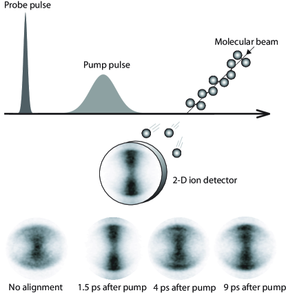
Figure 1: The figure shows a typical alignment experiment with short laser pulses. The cold thermal molecules are excited in a rotational state by a non-resonant pump pulse vertically polarized. After a time $t$ the molecules are coulomb-exploded with an intense, ultrashort probe pulse, also vertically polarized. The fragments recoil back-to-back and are imaged on a 2-D detector. The 3-D angular distributions can be found from these 2-D images because of the cylindrical symmetry. Four examples of experimental data with Iodobenzene are shown, where the imaged fragments are iodine ions: (from left) Probe applied long before pump, probe applied after respectively $1.5$, $4$ and $9$ps. Part of the anisotropy, which is directly apparent in the un-aligned case, is due to the coulomb-explosion preferentially occurring parallel to the probe polarization. This is corrected for when finding the 3-D distribution. Strictly speaking, Iodobenzene is an asymmetric top, but only slightly. For many purposes, it behaves like a symmetric top. Experimental data kindly provided by Simon S. Viftrup.

A typical example of an alignment experiment is shown in figure 1. Here, a rotationally cold supersonic molecular beam is used as the molecular system in a pump-probe experiment. The initial state is thus approximately a thermal state with only a few energy levels excited. The pump is a short, with a typical duration of a few picoseconds, intense non-resonant laser pulse, which induces the rotational state. The pump pulse is linearly polarized and since the initial state is thermal and therefore rotationally symmetric, the rotational state formed will be cylindrically symmetric around the pump polarization axis. Furthermore, the field mainly interacts with the molecule through the molecular polarizability, making the rotational state reflection symmetric in a plane orthogonal to the pump polarization. This last symmetry is not, however, a requirement for the tomographic method below.

After a delay, the molecules are coulomb-exploded by an intense ultrashort probe-pulse, polarized parallel to the pump pulse, and with a duration of typically some tens of femtoseconds. The molecular fragments recoil approximately back-to-back and their angular distribution can be found from the imaged fragments. Because of the cylindrical symmetry, the true angular distribution can be found even though the fragments are pulled by an electric field towards a detection plane containing the laser polarizations. It is the purpose of this paper to present a tomographic method to reconstruct the rotational quantum state of the system from the measurement data in such experiments.

We arrange the paper as follows: In section II we give a brief introduction to quantum state tomography. In section III we present the tomographic method for the rigid linear rotor. In section IV we show how to extend the tomographic method to molecules where centrifugal distortion must be taken into account. In section V we extend the tomographic method to the case of symmetric top molecules. In section VI we discuss the possibilities of recording the experimental data necessary to perform a reconstruction and we conclude the paper.

II Quantum state tomography

Mathematically, tomography is a technique, closely related to Fourier transformation, by which one can find a function from knowing its projection along all rotated lines. It found its first application in physiology in the 1970s, and tomographic techniques are now used extensively in hospital scanners, where images of internal tissue can be found from data recorded using X-rays or NMR. Apart from physiology, tomography is currently also being used in many other fields of research, including quantum physics and chemistry. Here the aim is to use measurements to find the quantum state of a system. The measurements are often taken to be spatial probability distributions at different times, which for harmonic oscillator systems makes the method very similar to the scanning methods from physiology invradon , invradon2 . Quantum state reconstruction has also been considered for many other systems including particles in traps (neutral atoms Buzekatom and ions Wineland ), general one-dimensional systems LeonhardtRaymerprl , dissociating molecules Juhl and the angular state of an electron in a Hydrogen atom with $n=3$ nlig3angmomtom .

III Reconstruction method for linear molecules

In this section we will present a reconstruction method by which one can find the rotational state of a linear rigid rotor. As usually in quantum tomography, we imagine that we are able to perform measurements of spatial distributions at different points of time and that we know the Hamiltonian governing the time evolution. The goal shall be to find the unique quantum state corresponding to these measurements.

III.1 Free rotation

Before discussing the description of the quantum state, we shall first digress to account for what we know about the Hamiltonian and its eigenstates. As discussed in the introduction, we are varying the time elapsed between the rotational state is created by a pump pulse and it is probed. During this time the molecule is in a field-free environment. Consequently, we shall be interested in the Hamiltonian for the free rotor.

The Hamiltonian governing the time evolution for the linear rotor with moment of inertia $\mathcal{I}$ is:

$$\hat{H}=\frac{\hat{\bm{J}}^{2}}{2\mathcal{I}},$$

where $\hat{\bm{J}}$ is the angular momentum operator. The energy eigenstates of this Hamiltonian are $\{|J,m\rangle\}$ where the angular momentum quantum number $J\in\mathbb{N}_{0}$ and the projection quantum number $m\in\{-J,-J+1,\ldots,J\}$. These states have energy $E_{J}=\hbar\Omega J(J+1)$, where $\Omega=\frac{\hbar}{2\mathcal{I}}$. Since we will attempt to reconstruct the quantum state using angular distribution measurements only, we shall need the spatial coordinate representation of the energy eigenstates. As discussed further below, we shall restrict our study to azimuthally symmetric distributions, and we shall hence be interested in the distribution of the polar angle $\theta$. For notational simplicity, we shall use the parameter $x=\cos(\theta)$ so the position representation of the eigenstates becomes:

$${}_{t}\langle x|J,m\rangle = \mathcal{P}_{J}^{m}(x)\,e^{-i\Omega J(J+1)t}.$$ (1)

There should be a factor of $e^{im\phi}$ in Eq. (1), but we can safely ignore this since we shall restrict our treatment to fixed values of $m$ . The $\mathcal{P}_{J}^{m}$ are the normalized associated Legendre polynomials, normalized on $x\in[-1,1]$ arfkenweber :

$$\int_{-1}^{1}dx\,\mathcal{P}^{m}_{J_{1}}(x)\mathcal{P}^{m}_{J_{2}}(x) = \delta_{J_{1},J_{2}}.$$ (2)

The multiplicative factors relating these to the un-normalized associated Legendre polynomials $P_{J}^{m}(x)$ are:

$$\mathcal{P}_{J}^{m}(x) = \sqrt{\frac{2J+1}{2}\,\frac{(J-m)!}{(J+m)!}}P_{J}^{m}(x).$$

Eq. (1) fully accounts for the free time evolution of the rotor. The angular position distribution of a single eigenstate is constant in time, but due to the different time dependent phase factors, a linear combination of different $|J,m\rangle$ states will have time dependent interference terms. Hence, such a linear combination will have a time dependent position distribution, also in the field free case.

After this brief account of the dynamics of the system, we proceed to define what we mean by the quantum state we are trying to reconstruct.

In the present treatment, the state will be characterized by its density operator $\hat{\rho}$, which allows a description of statistically mixed states. Specifically, we shall find all the matrix elements of $\hat{\rho}$ in the $|J,m\rangle$-basis at $t=0$ restricted to single $m$’s. This is the same as finding the diagonal blocks of constant $m$ in the density matrix, i.e. $\rho(J,m,J^{\prime},m)=\rho_{m}(J,J^{\prime})$. For a general state this is only a partial characterization, but if it is somehow known that the state has no correlations between different $m$ values, knowledge of all $\rho_{m}(J,J^{\prime})$ amounts to a full characterization of the state. This is the case in the experiment described in the introduction and the procedure below will completely reconstruct the quantum state for such systems. For the angular distribution, this diagonality in $m$ implies cylindrical symmetry for all time around a laboratory fixed axis, which we choose to be a spherical polar axis.

III.2 Measurements and observables

Having described the physical system, we proceed to consider the measurements performed; namely the (angular) position distribution measurements at the time $t$:

$$\textnormal{Pr}(x,t) = {}_{t}\langle x|\hat{\rho}_{m}|x\rangle_{t}$$ (3)

$$= \sum_{J_{1}=|m|}^{\infty}\sum_{J_{2}=|m|}^{\infty}{}_{t}\langle x|J_{1},m\rangle\langle J_{1},m|\hat{\rho}_{m}|J_{2},m\rangle\langle J_{2},m|x\rangle_{t}$$

$$= \sum_{J_{1}=|m|}^{\infty}\sum_{J_{2}=|m|}^{\infty}\rho_{m}\left(J_{1},J_{2}\right)\mathcal{P}^{m}_{J_{1}}(x)\mathcal{P}^{m}_{J_{2}}(x)\times$$

$$\qquad\qquad\quad\,\,\,e^{-i\Omega\left[J_{1}(J_{1}+1)-J_{2}(J_{2}+1)\right]t},$$

where $t=0$ is an arbitrary, but fixed, point of time after passage of the pump pulse. Our aim is to invert this equation to find the density matrix in the eigenstate-representation $\rho_{m}(J_{1},J_{2})$. It will prove convenient to write the products of the two Legendre polynomials $\mathcal{P}^{m}_{J_{1}}(x)\mathcal{P}^{m}_{J_{2}}(x)$ as a sum of single Legendre polynomials. This is exactly what is done in the decomposition of direct product bases for irreducible representations of the rotation group:

$$\mathcal{P}^{m}_{J_{1}}(x)\mathcal{P}^{m}_{J_{2}}(x) = \sum_{L=|J_{1}-J_{2}|}^{J_{1}+J_{2}}\sqrt{2\pi}\,C(J_{1},J_{2},L|m,-m,0)\mathcal{P}^{0}_{L}(x),$$ (4)

where $C(J_{1},J_{2},L|m,-m,0)$ are Clebsch-Gordan coefficients arfkenweber . Next, we introduce the variables $J=J_{1}+J_{2}$ and $\Delta J=J_{1}-J_{2}$, and the notational simplification:

$$C_{J,\Delta J,L}^{m} = \sqrt{2\pi}\,C\left(\frac{J+\Delta J}{2},\frac{J-\Delta J}{2},L\Big{|}m,-m,0\right).$$

Writing the position distributions Eq. (3) in the new variables $J$ and $\Delta J$, and using Eq. (4) we arrive at:

$$\textnormal{Pr}(x,t) = \left(\sum_{\begin{subarray}{c}J=|m|\\ \textnormal{$J$ even}\end{subarray}}^{\infty}\,\sum_{\begin{subarray}{c}\Delta J=-J\\ \textnormal{$\Delta J$ even}\end{subarray}}^{J}+\sum_{\begin{subarray}{c}J=|m|\\ \textnormal{$J$ odd}\end{subarray}}^{\infty}\,\sum_{\begin{subarray}{c}\Delta J=-J\\ \textnormal{$\Delta J$ odd}\end{subarray}}^{J}\right)\times$$ (5)

$$\rho_{m}\left(\frac{J+\Delta J}{2},\frac{J-\Delta J}{2}\right)\times$$

$$e^{-i\Omega\Delta J\left(J+1\right)t}\sum_{L=|\Delta J|}^{J}\mathcal{P}^{0}_{L}(x)C^{m}_{J,\Delta J,L}.$$

For readability, we shall in the following abbreviate the summations in the first line of Eq. (5) as:

$$\sum_{J,\,\Delta J}^{ee,oo}.$$ (6)

We have now expanded the time dependent position distribution on orthogonal polynomials $\mathcal{P}_{\alpha}^{0}(x)$ with coefficieents that can be found by simple spatial integrals $\int_{-1}^{1}dx\mathcal{P}_{\alpha}^{m}(x)\textnormal{Pr}(x,t)$. These coefficients, in turn, are linear combinations of the density matrix elements which can be found if the distribution is recorded at different times, as we show below.

III.3 Reconstruction formulas

In this subsection we will present the reconstruction formulas. We will first consider the off-diagonal elements of the density matrix and deal with the diagonal elements further below.

III.3.1 Reconstruction of off-diagonal elements

We let $N_{T}T$ be the time interval in which position measurements $\textnormal{Pr}(x,t)$ have been performed. Here $N_{T}\in\mathbb{N}$ and the minimum measurement time $T=2\pi\mathcal{I}/\hbar$, equalling $\sqrt{2}$ times the semiclassical rotational period of the $J=1$ state or the rotational revival period rotrevival .

The time dependent factor $e^{-i\Omega\Delta J(J+1)t}$ in Eq. (5) suggests that a temporal Fourier transform evaluated at frequency $\Omega\beta(\alpha+1)$, with $\alpha$ and $\beta$ suitably chosen integers, will be part of the reconstruction procedure. Following this strategy, we consider the integral:

$$I(\alpha,\beta)=\frac{1}{N_{T}T}\int_{0}^{N_{T}T}dt\,e^{i\Omega\beta(\alpha+1)t}\int_{-1}^{1}dx\,\mathcal{P}^{0}_{\alpha}(x)\textnormal{Pr}(x,t)$$

$$=\sum_{J,\,\Delta J}^{ee,oo}\rho_{m}\left(\frac{J+\Delta J}{2},\frac{J-\Delta J}{2}\right)\delta_{\beta(\alpha+1)-\Delta J(J+1)}\times$$

$$\sum_{L=|\Delta J|}^{J}C^{m}_{J,\Delta J,L}\delta_{L,\alpha},\qquad$$ (7)

where $\alpha\in\{|m|,|m+1|,\ldots\}$ and $\beta\in\{-\alpha,-\alpha+2,\ldots,\alpha\}$, which makes both $\alpha$ and $\beta$ are either even or odd. For the time being, we shall choose $\beta\neq 0$ and deal with the $\beta=0$ case (i.e. diagonal matrix elements) later.

Notice that the delta-function in the sum over $L$ ensures that $\alpha$, $J$ and $\Delta J$ are all of the same parity. This is also the parity of $\beta$, since we chose $\alpha$ and $\beta$ to be of the same parity.

$$I(\alpha,\beta) = \sum_{\begin{subarray}{c}J=|m|\\ \textnormal{parity as $\alpha$}\end{subarray}}^{\infty}\sum_{\begin{subarray}{c}\Delta J=-J\\ \textnormal{parity as $\alpha$}\end{subarray}}^{J}\rho_{m}\left(\frac{J+\Delta J}{2},\frac{J-\Delta J}{2}\right)\times$$ (8)

$$\delta_{\beta(\alpha+1)-\Delta J(J+1)}C^{m}_{J,\Delta J,\alpha}\sum_{L=|\Delta J|}^{J}\delta_{L,\alpha}.$$

Rather than giving a single term in the general case, the sums are greatly simplified. From the $L$-sum we get $I(\alpha,\beta)=0$ unless:

$$\left|\Delta J\right|\leq \alpha \leq J.$$ (9)

Using this in conjunction with the other delta-function we find $I(\alpha,\beta)=0$ unless:

$$|\Delta J|\leq|\beta|\leq\alpha,\quad\textnormal{$\beta$ and $\Delta J$ of same sign}.$$ (10)

Furthermore, this delta-function demands:

$$\beta\left(\alpha+1\right) = \Delta J\left(J+1\right).$$ (11)

As it turns out, for many choices of $\alpha$ and $\beta$ there is only the straightforward solution to the equation Eq. (11) under the conditions Eqs. (9) and (10), namely $\alpha=J$ and $\beta=\Delta J$. In these cases we easily find the density matrix elements:

$$I\left(\alpha,\beta\right) = C^{m}_{\beta,\alpha,\alpha}\,\rho_{m}\left(\frac{\alpha+\beta}{2},\frac{\alpha-\beta}{2}\right),\,\begin{subarray}{c}\textnormal{unique solution}\\ \textnormal{to \ref{eq:beting1}, \ref{eq:beting2} and \ref{eq:stordelta}.}\end{subarray}$$ (12)

For some choices of $\alpha$ and $\beta$ there will be more than one term surviving from the sums in Eq. (8). The physical reason for this is that there is more than one pair of energy eigenstates having a certain energy difference. One example is the energy difference between the states $(J_{1}=3\rightarrow J_{2}=0)$ and between the states $(J_{1}=6\rightarrow J_{2}=5)$. In our variables this corresponds to $(J=3,\Delta J=3)$ and $(J=11,\Delta J=1)$. We proceed to show that all density matrix elements with $\beta\neq 0$ can be found regardless of this complication.

Imagine that we have found $I(\alpha,\beta)$ to contain the term $C^{m}_{\beta,\alpha,\alpha}\,\rho_{m}\left(\frac{\alpha+\beta}{2},\frac{\alpha-\beta}{2}\right)$, but also several other terms $C^{m}_{\beta^{\prime}_{n_{1}},\alpha^{\prime}_{n_{1}},\alpha}\,\rho_{m}\left(\frac{\alpha^{\prime}_{n_{1}}+\beta^{\prime}_{n_{1}}}{2},\frac{\alpha^{\prime}_{n_{1}}-\beta^{\prime}_{n_{1}}}{2}\right)$, where $n_{1}=1,2,\ldots,N_{1}$. The strategy is to calculate all the integrals $I(\alpha_{n_{1}}^{\prime},\beta_{n_{1}}^{\prime})$. These may also contain several terms with $(J=\alpha^{\prime\prime}_{n_{2}},\Delta J=\beta_{n_{2}}^{\prime\prime})$, where $n_{2}=1,2,\ldots,N_{2}$, but always fewer than in the former integrals, i.e. $N_{j}<N_{j+1}$. The reason for this is the condition $|\Delta J|\leq|\beta|$ from Eq. (10): Whereas the $\beta=\Delta J$ term will always appear, the rest of the terms in the sum Eq. (8) will have $\Delta J<\beta$, whereby the procedure will terminate and we can find all the matrix elements of $\hat{\rho}_{m}$ by back substitution. If one is interested only in matrix elements up to some maximum $J=J_{max}$ it is only necessary to search for degeneracies in the energy differences for all $(J,\beta)$ up to $J=J_{max}(J_{max}+1)/2$ for even $J_{max}$ and $J_{max}(J_{max+1})$ for odd $J_{max}$.

To clarify this procedure a little, let us consider an example: We shall choose $m=0$ and try to find the matrix element $\rho_{0}(5,0)$. In this case $J=\Delta J=5$, and we find $I(5,5)=C^{m}_{5,5,5}\rho_{m}(5,0)+C^{m}_{9,3,5}\rho_{m}(6,3)+C^{m}_{29,1,5}\rho_{m}(15,14)$. To find the desired matrix element we shall need the two extra equations $I(9,3)=C^{m}_{9,3,3}\rho_{m}(6,3)+C^{m}_{29,1,3}\rho_{m}(15,14)$ and $I(29,1)=C^{m}_{29,1,1}\rho_{m}(15,14)$. These three resulting equations can now be solved by back substitution to yield $\rho_{m}(5,0)$, $\rho_{m}(6,3)$ and $\rho_{m}(15,14)$.

III.3.2 Reconstructing the diagonal

We proceed to show how one can go about finding the diagonal of $\hat{\rho}_{m}$ in the energy-representation. To do this we shall use Eq. (8) with $\beta=0$, by which $\alpha$ is even:

$$I(\alpha,0) = \frac{1}{N_{T}T}\int_{0}^{N_{T}T}dt\,\int_{-1}^{1}dx\,\mathcal{P}^{0}_{\alpha}(x)\textnormal{Pr}(x,t)$$ (13)

$$= \sum^{\infty}_{\begin{subarray}{c}J=|m|\\ \textnormal{$J$ even}\end{subarray}}\rho_{m}\left(\frac{J}{2},\frac{J}{2}\right)C^{m}_{J,0,\alpha}$$

$$= \sum^{\infty}_{J_{1}=|m|}\rho_{m}\left(J_{1},J_{1}\right)C^{m}_{2J_{1},0,\alpha},$$

where we have used $J_{1}=J/2$. We notice that the coefficient $C^{m}_{2J_{1},0,\alpha}$ is zero unless $\alpha\leq 2J_{1}$. We arrange the $I(\alpha,0)$ in a column vector $\bm{I}$ and the $\rho_{m}(J_{1},J_{1})$ in a column vector $\bm{R}$:

$$\bm{I} = \left(\begin{array}[]{c}I\left[2|m|,0\right]\\ I\left[2(|m|+1),0\right]\\ \vdots\end{array}\right),$$ (17)

$$\bm{R} = \left(\begin{array}[]{c}\rho_{m}(|m|,|m|)\\ \rho_{m}(|m|+1,|m|+1)\\ \vdots\end{array}\right).$$ (21)

Eq. (13) now reads:

$$\bm{I} = \mathscr{M}\cdot{\bm{R}},\qquad\textnormal{where}$$ (22)

$$\mathscr{M} = \underbrace{\left(\begin{array}[]{c c c}C^{m}_{2|m|,0,2|m|}&C^{m}_{2(|m|+1),0,2|m|}&\ldots\\ 0&C^{m}_{2(|m|+1),0,2(|m|+1)}&\ldots\\ \vdots&\vdots&\ddots\end{array}\right)}_{upper-triangular}$$ (26)

To find the desired elements $\rho_{m}(J_{1},J_{1})$ we shall need to invert the matrix $\mathscr{M}$, which can be done since the diagonal elements $C^{m}_{\alpha,0,\alpha}=\sqrt{2\pi}C(\alpha/2,\alpha/2,\alpha|m,-m,0)$ are all non-zero. In practical applications, one may truncate the linear system at some maximum $J_{1}$ corresponding to a maximum energy.

It may be noted that since the linear system (17) always has the same coefficient matrix, we could just has well have used a function $\mathcal{F}_{J_{1}}$ that selects a certain $J_{1}$ in (13), so that:

$$\rho_{m}(J_{1},J_{1}) = \frac{1}{N_{T}T}\int_{0}^{N_{T}T}dt\,\int_{-1}^{1}dx\,\mathcal{F}_{J_{1}}(x)\textnormal{Pr}(x,t).$$

The $\mathcal{F}_{J_{1}}(x)$ can be precalculated and are given by:

$$\mathcal{F}_{J_{1}}(x) = \sum_{J=J_{1}}^{\infty}f_{J_{1},J}\mathcal{P}_{2J}(x),$$

where the expansion coefficients $f_{J_{1},J}$ are easily found by Cramer’s rule and the fact that $\mathscr{M}$ is upper-triangular:

$$f_{J_{1},J}=(-1)^{J_{1}+J}\frac{\left|\mathscr{M}^{\textnormal{sub}}_{J_{1},J}\right|}{\prod_{\gamma=J_{1}}^{J}\mathscr{M}(\gamma,\gamma)},$$ (27)

and $\left|\mathscr{M}^{\textnormal{sub}}_{J_{1},J}\right|$ is the determinant of the sub-matrix:

$$\mathscr{M}^{\textnormal{sub}}_{J_{1},J} = \mathscr{M}\left(J_{1}+1:J_{1}+1+J,J_{1}+2:J_{1}+2+J\right).$$

This method would be relevant if only a few particular elements of the density matrix are desired. One may notice the similarity of these functions to the pattern functions used with harmonic oscillator systems patternfunc ,pattern2 .

It may be noted that we could not have circumvented the back substitution procedure in section III.3.1 by choosing other functions than the $\mathcal{P}^{0}_{\alpha}(x)$ in Eq. (8), since the solution of the resulting system of equations depends on the measurement values through the $I(\alpha_{j},\beta_{j})$’s.

IV Real molecules and centrifugal distortion

In the above treatment we used the rigid rotor Hamiltonian $\hat{H}=\frac{\hat{\bm{J}}^{2}}{2\mathcal{I}}$, whereas terms of higher order in $\hat{\bm{J}}^{2}$ will be important in real molecules in highly excited rotational states. With the lowest order centrifugal distortion the Hamiltonian is instead:

$$\hat{H}^{\prime} = \frac{\hat{\bm{J}}^{2}}{2\mathcal{I}}-\frac{D\hat{\bm{J}}^{4}}{\hbar^{3}}.$$

The states $|J,m\rangle$ are still the energy eigenstates, but here with energy $E_{J}=\hbar\Omega J(J+1)-\hbar DJ^{2}(J+1)^{2}$. The constant $D\propto\frac{1}{\mathcal{I}^{3}\omega^{2}}$, where $\omega$ is the harmonic frequency of the molecular bond. The reconstruction strategy is similar to the one in Eq. (III.3.1):

$$I_{CD}(\alpha,\beta) = \lim_{T\rightarrow\infty}\frac{1}{T}\int_{0}^{T}dt\,e^{i\beta(\alpha+1)\left[\Omega-D\beta(\alpha+1)\right]t}\times$$ (28)

$$\quad\qquad\int_{-1}^{1}dx\,\mathcal{P}^{0}_{\alpha}(x)\textnormal{Pr}(x,t).$$

In this case, the conditions Eqs. (9) and (10) still apply, but Eq. (11) is replaced by:

$$\beta(\alpha+1)-\frac{D}{\Omega}\beta^{2}(\alpha+1)^{2}=\quad$$

$$\Delta J(J+1)-\frac{D}{\Omega}{\Delta J}^{2}\left(J+1\right)^{2}.$$ (29)

Depending on the value of $D/\Omega$, there may be more than one set of $(\Delta J,J)$ that satisfies the conditions Eqs. (9)-(10) and Eq. (IV), but it will usually be much fewer than in the rigid rotor case. Consequently, one can often avoid the back substitution procedure above and use $I_{CD}(\alpha,\beta)=C^{m}_{\beta,\alpha,\alpha}\,\rho_{m}\left(\frac{\alpha+\beta}{2},\frac{\alpha-\beta}{2}\right)$.

V Symmetric top states

Having treated the linear rotor case, we will now straightforwardly generalize the results from section III to symmetric top molecules. This class contains many more molecules than the linear class.

The eigenvectors of the Hamiltonian are in this case the set $\{|Jkm\rangle\}$ with associated energy $E=\hbar\Omega_{1}J(J+1)-\hbar\Omega_{2}k^{2}$. Here $k$ is the quantum number for the projection of the angular momentum on the symmetry axis of the molecule, where $m$ was associated with a projection on a space-fixed axis. Like $m$, $k$ can assume the values $-J,-J+1,\ldots,J$. For a linear molecule $k=0$, and the treatment in section III can indeed be seen as a special case of the symmetric top. In accordance with the above treatment we shall assume that we can measure the polar angular distribution, parametrized by $x=\cos(\theta)$, for a certain value of $k$ and $m$. The angular position representations of the eigenstates are:

$${}_{t}\langle x|Jkm\rangle = \sqrt{\frac{2J+1}{2}}d^{J}_{km}(x)e^{-i(\Omega_{1}J(J+1)-\Omega_{2}k^{2})},$$

where the $d^{J}_{km}(x)$ are the usual rotation matrix elements, and the eigenstates are normalized on $[-1,1]$. The quantities $\Omega_{1}=1/2\mathcal{I}_{x}$ and $\Omega_{2}=\hbar/(2\mathcal{I}_{z}-2\mathcal{I}_{x})$. Here we have chosen the $z$ axis as the molecular symmetry axis, and used that the moments of inertia $\mathcal{I}_{x}=\mathcal{I}_{y}$. As in Eq. (1), we can safely ignore the dependence of the two other Euler angles $\phi$ and $\chi$, since we are working in the subspace of fixed $k$ and $m$. We can now readily generalize the treatment in section III by exchanging the functions $\mathcal{P}_{J}^{m}(x)$ with $\sqrt{(2J+1)/2}\,d^{J}_{km}(x)$ and the lower summation indices $|m|$ with $M_{km}=\textnormal{max}(|m|,|k|)$. In particular, Eq. (3) generalizes to:

$$\textnormal{Pr}(x,t) = {}_{t}\langle x|\hat{\rho}_{k,m}|x\rangle_{t}$$ (30)

$$= \sum_{\begin{subarray}{c}J_{1}=\\ M_{km}\end{subarray}}^{\infty}\sum_{\begin{subarray}{c}J_{2}=\\ M_{km}\end{subarray}}^{\infty}\rho_{m}\left(J_{1},J_{2}\right)d^{J_{1}}_{km}(x)d^{J_{2}}_{km}(x)\times$$

$$\sqrt{\frac{(2J_{1}+1)(2J_{2}+1)}{4}}e^{-i\Omega\left[J_{1}(J_{1}+1)-J_{2}(J_{2}+1)\right]t}.$$

Products of the functions $d^{J}_{km}$(x) can again be decomposed into linear combinations of single Legendre polynomials, again introducing $J=(J_{1}+J_{2})/2$ and $\Delta J=(J_{1}-J_{2})/2$ tinkham , Sakurai-san :

$$\sqrt{\frac{(2J_{1}+1)(2J_{2}+1)}{4}}d^{J_{1}}_{km}(x)d^{J_{2}}_{km}(x) =$$

$$\sum_{L=|J_{1}-J_{2}|}^{J_{1}+J_{2}}C^{km}_{J,\Delta J,L}\mathcal{P}_{L}^{0}(x),$$ (31)

where

$$C^{km}_{J,\Delta J,L} = \sqrt{\frac{2}{2L+1}}C(J_{1},J_{2},L|m,-m,0)\times$$ (32)

$$\,\qquad\qquad C(J_{1},J_{2},L;k,-k,0).$$

Proceeding as in section III, we calculate the integrals $I(\alpha,\beta)$ and arrive at the equivalent of Eq. (8):

$$I(\alpha,\beta) = \sum_{\begin{subarray}{c}J=M_{km}\\ \textnormal{parity as $\alpha$}\end{subarray}}^{\infty}\,\sum_{\begin{subarray}{c}\Delta J=-J\\ \textnormal{parity as $\alpha$}\end{subarray}}^{J}\rho_{k,m}\left(\frac{J+\Delta J}{2},\frac{J-\Delta J}{2}\right)\times$$ (33)

$$\delta_{\beta(\alpha+1)-\Delta J(J+1)}C^{km}_{J,\Delta J,\alpha}\sum_{L=|\Delta J|}^{J}\delta_{L,\alpha}.$$

The reconstruction of the matrix elements $\rho_{k,m}(J_{1},J_{2})$ can therefore be done like in sections III.3.1 and III.3.2, where one uses the $C^{km}_{J,\Delta J,L}$ defined in Eq. (32) instead of $C^{m}_{J,\Delta J,L}$.

VI Discussion

As the reader may have noticed, the method above effectively deals with a semi-continuous one-dimensional reconstruction in the space of $x$ and $J$, and not with the reconstruction of a general state. The reason for this limitation is that the inversion formulas we are using are integral transformations that preserve dimensionality, like e.g. the Fourier transformation in $t$ in Eq. (8). If the dimensionality of the measurements are not at least as large as the dimensionality of the quantum state, such an approach nearly always fails uspiselig . For example, in one dimension the density matrix is a two-dimensional object $\langle x|\hat{\rho}_{k,m}|x^{\prime}\rangle$ which has the same dimensionality as the measurement-space $\textnormal{Pr}(x,t)$. In contrast, the full quantum state of e.g. the linear rotor is a four-dimensional object $\langle x,\phi|\hat{\rho}|x^{\prime},\phi^{\prime}\rangle$, while the angular measurements $\textnormal{Pr}(x,\phi,t)$ would only be three-dimensional. If one desired to reconstruct a full general quantum state, one would either have to be able to perform more advanced measurements or to vary the Hamiltonian as suggested in raymervarham . Because of the difficulty of precisely knowing Hamiltonians arising from e.g. additional laser pulses, we have instead treated the one-dimensional system using only routinely performed measurements.

In spite of this limitation, the situation where the one-dimensional description is a complete characterization of the quantum system is experimentally common. Indeed, for the situation described in the introduction, there are no correlations between the different $k$ and $m$ quantum numbers. The question is of course whether one can perform measurements of polar angular distributions for certain $k$ and $m$ quantum numbers.

A conceptually straightforward solution would be to use very low-temperature samples, where only $k=m=0$ is populated before the interaction with the pump pulse. Note that this would not imply that the created rotational state would be a pure state due to inhomogeneities in the pump pulse focus, e.g. the pump intensity generally varies over the focus or shot-to-shot variation of laser intensity. Though conceptually simple, this situation is unpractical due to the smallness of the rotational energies demanding very low temperatures.

A more practical approach would be to select a certain value of $k$ and $m$ before interaction with the pump pulse. For polar symmetric top molecules this can be done for certain values of $k$ and $m$ by using the linear Stark effect through hexapole focusing techniques henriksref10 , hexia . The linear Stark shift for symmetric tops is ${\Delta E^{(1)}=-\mu\varepsilon km/J(J+1)}$, where $\mu$ is the dipole moment and $\varepsilon$ is the magnitude of the electric field. Since one starts out with a thermal sample, there are no correlations in either $J$, $k$ or $m$ in the state before interactions with the pump. Therefore, one does not discard any information on the state by picking out all sets of values of $J$, $k$ and $m$ one by one. If the molecular beam was sufficiently cold, one could select components of the beam with certain $k$ and $m$ values, as is required by the method above. One would then also select a certain value of $J$, which is not required, but on the other hand poses no problem. Furthermore, the apparent ambiguity that a change of sign of both $k$ and $m$ gives the same Stark shift is of no consequence, since the state created by the pump has identical matrix elements $\rho_{k,m}(J,J^{\prime})$ and $\rho_{-k,-m}(J,J^{\prime})$ due to the invariance of the initial state and of the pump-pulse interaction Hamiltonians under the interchange $(k,m)\rightarrow(-k,-m)$.

Most linear molecules and symmetric tops with $k=0$ do not exhibit any linear Stark shift Flemmingbog , but also here hexapole focusing techniques can be used to select specific values of $J$ and $m$ through the second order Stark shift. Here, both molecules with the quantum numbers $(J,m)$ and $(J,-m)$ are selected, but this is of no consequence since $\rho_{m}(J,J^{\prime})=\rho_{-m}(J,J^{\prime})$ in accord with the previous paragraph.

In conclusion, we have presented a method to reconstruct the blocks $\rho_{k,m}(J,J^{\prime})$ of the rotational density matrix for linear and symmetric top molecules from angular distributions. This amounts to a complete characterization of the quantum state in a common experimental setup. Finally, we have suggested how the required measurements could be performed with existing techniques.

- (1) F. Rosca-Pruna and M. J. J. Vrakking, Revival structures in picosecond laser-induced alignment of I2 molecules. I. Experimental results, J. Chem. Phys. 116, p. 6567-6578 (2002).
- (2) H. Stapelfeldt and T. Seideman, Colloquium: Aligning molecules with strong laser pulses, Rev. Mod. Phys. 75, p. 543-557 (2003).
- (3) P. W. Dooley, I. V. Litvinyuk, K. F. Lee, D. M. Rayner, M. Spanner, D. M. Villeneuve, and P. B. Corkum, Direct imaging of rotational wave-packet dynamics of diatomic molecules, Phys. Rev. A 68, 023406, p. 1-12 (2003).
- (4) E. Péronne, M. D. Poulsen, H. Stapelfeldt, C. Z. Bisgaard, E. Hamilton and T. Seideman, Nonadiabatic laser-induced alignment of iodobenzene molecules, Phys. Rev. A 70, 063410/1-9 (2004).
- (5) J. Itatani, J. Levesque, D. Zeidler, H. Niikura, H. Pépin, J. C. Kieffer, P. B. Corkum and D. M. Villeneuve, Tomographic imaging of molecular orbitals, Nature 432, p. 867 (2004).
- (6) K. Vogel and H. Risken, Determination of quasiprobability distributions in terms of probability distributions for the rotated quadrature phase, Phys. Rev. A 40, p. R2847-2849 (1989)
- (7) J. Bertrand and P. Bertrand, A tomographic approach to Wigner’s function, Found. Phys. 17, p.397-405 (1987)
- (8) G. Drobný and V. Bužek, Reconstruction of motional states of neutral atoms via MaxEnt principle, arXiv: quant-ph/0202080 v1. (2002).
- (9) D. Leibfried, D. M. Meekhof, B. E. King, C. Monroe, W. M. Itano, and D. J. Wineland, Experimental Determination of the Motional Quantum State of a Trapped Atom, Phys. Rev. Lett. 77, p. 4281-4285 (1996).
- (10) U. Leonhardt and M. G. Raymer, Observation of Moving Wave Packets Reveals Their Quantum State, Phys. Rev. Lett. 76, p. 1985-1989 (1996).
- (11) E. Skovsen, H. Stapelfeldt, S. Juhl, K. Mølmer, Quantum state tomography of dissociating molecules, Phys. Rev. Lett. 91, 9, 090406/1-4 (2003)
- (12) J. R. Ashburn, R. A. Cline, P. J. M. van der Burgt, W. B. Westerveld and J. S. Risley, Experimentally determined density matrices for H formed in H+-He collisions from to keV Phys. Rev. A 41, p. 2407-2421 (1990).
- (13) S. S. Safonov, Tomography of Quantum Spinor States, arXiv:quant-ph/9807031, p. 1-15 (1998).
- (14) G. B. Arfken and H. J. Weber, Mathematical methods for physicists, 5th ed., Academic Press, San Diego (2001).
- (15) G. M. D´Ariano, C. Macchiavello and M. G. A. Paris, Detection of the density matrix through optical homodyne tomography without filtered back projection, Phys. Rev. A 50, p. 4298-4303 (1994).
- (16) U. Leonhardt, H. Paul and G. M. D´Ariano, Tomographic reconstruction of the density matrix via pattern functions, Phys. Rev. A 52, p. 4899-4907 (1995).
- (17) M. Tinkham, Group Theory and Quantum Mechanics, McGraw-Hill, New York (1964).
- (18) J. J. Sakurai, Modern Quantum Mechanics, Addison- Wesley, (1994).
- (19) A. S. Mouritzen and K. Mølmer, Tomographic reconstruction of quantum states in spatial dimensions, arXiv:quant-ph/0511173 (2005).
- (20) M. G. Raymer, M. Beck and D. F. McAlister, Complex Wave-Field Reconstruction Using Phase-Space Tomography, Phys. Rev. Lett. 72, p. 1137-1140 (1994).
- (21) D. H. Parker and R. B. Bernstein, Oriented Molecule Beams via the Electrostatic Hexapole: Preparation, Characterization, and Reactive Scattering, Annu. Rev. Phys. Chem. 40, p. 561-595 (1989).
- (22) S. R. Gandhi and R. B. Bernstein, Focusing and state selection of NH3 and OCS by the electrostatic hexapole via first- and second-order Stark effects, J. Chem. Phys. 87, p. 6457-6467 (1987).
- (23) J. E. Wollrab, Rotational Spectra and Molecular Structure, Academic Press, London (1967).