Squeezing and entangling nuclear spins in helium 3

Abstract

We present a realistic model for transferring the squeezing or the entanglement of optical field modes to the collective ground state nuclear spin of ³He using metastability exchange collisions. We discuss in detail the requirements for obtaining good quantum state transfer efficiency and study the possibility to readout the nuclear spin state optically.

I Introduction

Helium 3 atoms in their ground state possess a purely nuclear spin $I=1/2$. Such spins are well-isolated from the environment and show extremely long coherence times. Longitudinal coherence times $T_{1}$ of several days are measured in room temperature samples Heil . The transverse coherence time $T_{2}$, which would be as long as $T_{1}$ in zero magnetic field, is usually limited by magnetic field inhomogeneity if no special precaution is taken. Transverse coherence times of several hours are observed in a very low field Cohen . These very long coherence times originate from the weakness of magnetic coupling on the one hand, and from the absence of electrical coupling on the other hand, as there is no electric quadrupole coupling within the ground state for spins 1/2. It is tempting to exploit such long-lived coherence for quantum information purposes. In a previous letter prl we studied the possibility to transfer the squeezing of a cavity mode to ³He nuclear spins. We showed that the squeezeing could be stored and retrieved from the atoms, thus realizing a quantum memory Fleishhauer ; molmer ; dantanpra04 ; vanderWal ; Schori ; Polzik . For the sake of simplicity we presented in our letter a simplified model involving only two sublevels in the metastable state and gave numerical results for the more complicated case of ³He. In this paper we concentrate on ³He and treat in detail this more realistic case.

Section II is devoted to metastability exchange collisions. We derive linearized Heisenberg-Langevin equations describing the exchange collisions from the standpoint of quantum fluctuations. In section III we describe the model for squeezing transfer from a squeezed vacuum mode of the electromagnetic field to the atoms. Numerical results are shown and discussed in section IV. In section V we obtain analytical results in the adiabatic elimination limit for the optical coherences and the cavity field. Section VI is devoted to the readout scheme of the quantum memory. In section VII, as a straightforward application of our scheme, we consider the possibility of creating long-lived quantum correlations between two macroscopic spins, in the move of the successful experiment in Copenhagen Polzik2 , in which two macroscopic spins were entangled for $0.5$ ms, but on a completely different timescale. Finally, in section VIII, we use a toy model to explore the consequences of an imperfect polarization of the atoms on our squeezing transfer scheme.

II Metastability exchange collisions in helium 3

Over forty years ago, Colegrove, Schearer and Walters CSW demonstrated a technique to polarize ³He relying on $(i)$ an optical interaction on an infrared transition from the metastable $2^{3}$S triplet state to the $2^{3}$P triplet state, and $(ii)$ metastability exchange collisions between atoms in the ground state and in the metastable state. During such a collision, two atoms exchange their electronic degrees of freedom so that the metastable atom, oriented by optical pumping and with a nuclear polarization due to hyperfine coupling in the metastable state, becomes a polarized ground state atom partridge . This technique called metastability exchange optical pumping is currently used to prepare polarized samples for nuclear physics experiments as well as in nuclear magnetic resonance imaging applications LeducReview .

In what follows we suggest that metastability exchange collisions can also be used to transfer quantum correlations to the ground state nuclear spin of ³He.

II.1 Equations for the one-body density matrix elements

Partridge and Series partridge describe a metastability exchange (ME) collision in terms of the one-body density matrices representing the internal states of two colliding atoms that we name $\rho^{\rm at}_{\rm g}$ and $\rho^{\rm at}_{\rm m}$ for the ground and metastable state, respectively. The density matrices after the collision, ${\rho^{\rm at}_{\rm g}}^{\prime}$ and ${\rho^{\rm at}_{\rm m}}^{\prime}$, are given by

$$\left\{\begin{array}[]{lcl}{\rho^{\rm at}_{\rm g}}^{\prime}&=&\textrm{Tr}_{e}\;\rho^{\rm at}_{\rm m}\\ {\rho^{\rm at}_{\rm m}}^{\prime}&=&\rho^{\rm at}_{\rm g}\otimes\textrm{Tr}_{n}\;{\rho^{\rm at}_{\rm m}}\\ \end{array}\right.$$ (1)

where $\textrm{Tr}_{e}$ and $\textrm{Tr}_{n}$ are trace operators over the electronic and nuclear variables.

Let us consider $n$ metastable and $N$ ground state independent atoms. We introduce $\rho_{\rm g}=N\rho^{\rm at}_{\rm g}$, $\rho_{\rm m}=n\rho^{\rm at}_{\rm m}$, and the same for $\rho_{\rm g}^{\prime}$ and $\rho_{\rm m}^{\prime}$.

To represent the state of the system, we will use the density matrix $\rho$ defined by:

$$\rho=\left(\begin{array}[]{cc}\rho_{\rm m}&0\\ 0&\rho_{\rm g}\\ \end{array}\right)$$ (2)

Note that $Tr{\rho}=n+N$ and that we neglect all coherences between the ground and the metastable states. The matrices $\rho_{\rm g}$ and $\rho_{\rm m}$ evolve according to

$$\left\{\begin{array}[]{lcl}\frac{d}{dt}\rho_{\rm g}&=&-\gamma_{f}\rho_{\rm g}+\gamma_{f}\rho_{\rm g}^{\prime}\\ \frac{d}{dt}\rho_{\rm m}&=&-\gamma_{m}\rho_{\rm m}+\gamma_{m}\;\rho_{\rm m}^{\prime}\end{array}\right.$$ (3)

where $\gamma_{f}$ and $\gamma_{m}$ are the metastability exchange collision rates in the ground and metastable states respectively

$$\gamma_{m}=N\gamma_{exc}\hskip 28.45274pt\gamma_{f}=n\gamma_{exc}$$ (4)

with $\gamma_{exc}$ a rate depending on the metastability exchange cross section, the relative velocity of the atoms and the volume explored by the atoms.

The calculation of $d\rho/dt$ is performed by expressing $\rho$ in the decoupled spin basis of the nuclear spin $I=\frac{1}{2}$ and the total electronic spin $J=S=1$ in the metastable state, followed by a projection onto the hyperfine states (eigenstates of the total momentum operator $F$ and $F_{z}$) which we name from $1$ to $6$ as in figure 1. The explicit evolution equations for the density matrix elements are given in the Appendix. The fully polarized state in which all the atoms are in the sublevel with highest angular momentum projection along $z$ is stationary for equations (3).

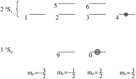
Figure 1: Sublevels $1$ to $6$ are metastable; $9$ and $0$ are the ground state sublevels. The fully polarized stationary state is shown.

Starting from equations (3) we proceed in two steps which will be detailed in the following:

1. We linearize these equations around the fully polarized steady state in which the only non-zero elements of $\rho$ are $\rho_{44}=n$ and $\rho_{00}=N$.

2. From the linearized classical equations, interpreted as semiclassical equations for the mean values of the collective operators, we derive the corresponding Heisenberg-Langevin equations.

II.2 Linearized Heisenberg-Langevin equations

By linearization around the fully polarized solution we obtain equations for the “fluctuations” or deviations of the $\rho_{ij}$ from their steady-state values. Such linear equations coincide with the linearized semiclassical equations for the collective atomic operators operators mean values:

$$\rho_{kl} = \langle S_{lk}\rangle\hskip 56.9055ptk,l=1,\ldots,6$$ (5)

$$\rho_{kl} = \langle I_{lk}\rangle\hskip 56.9055ptk,l=9,0$$ (6)

where $S_{kl}=\sum_{i=1}^{n}|k\rangle_{i}\langle l|_{i}$ for $k,l=1,\ldots,6$ and $I_{kl}=\sum_{i=1}^{N}|k\rangle_{i}\langle l|_{i}$ for $k,l=9,0$ are the collective atomic operators in the metastable and ground state, respectively. The corresponding linearized Heisenberg-Langevin equation for the operators are obtained by adding zero-mean valued fluctuating terms which are the Langevin forces. Denoting by $f_{\alpha}$ the Langevin force for the operator $\alpha$ we get a closed set of equations:

$$\dot{S}_{21} = -\gamma_{m}S_{21}+f_{21}$$ (7)

$$\dot{S}_{32} = \frac{2}{9}\gamma_{m}\left(-\frac{7}{2}S_{32}+\sqrt{3}S_{21}+S_{65}\right)+f_{32}$$ (8)

$$\dot{S}_{65} = -\frac{7}{9}\gamma_{m}\left(S_{65}-\frac{2}{7}\sqrt{3}S_{21}-\frac{2}{7}S_{32}\right)+f_{65}$$ (9)

$$\dot{S}_{43} = \gamma_{m}\left(-\frac{1}{3}S_{43}+\frac{2\sqrt{3}}{9}(S_{32}+S_{65})\right)+\frac{\sqrt{3}}{3}\gamma_{f}I_{09}+f_{43}$$ (10)

$$\dot{I}_{09} = \frac{1}{3}\left[-3\gamma_{f}I_{09}+2\gamma_{m}\left(S_{32}-\frac{1}{2}S_{65}+\frac{\sqrt{3}}{2}S_{43}+\frac{\sqrt{3}}{2}S_{21}\right)\right]+f_{09}$$ (11)

If $\alpha$ and $\beta$ denote two system operators, $\langle f_{\alpha}(t)f_{\beta}(t^{\prime})\rangle=D_{\alpha\beta}\delta(t-t^{\prime})$ where $D_{\alpha,\beta}$ is the corresponding coefficient of the diffusion matrix which can be calculated using the generalized Einstein relations CohenBook for an ensemble of uncorrelated atoms. The non-zero coefficients are

$$D_{43,34}=\frac{2}{3}\gamma_{m}n$$, , .

(12)

Langevin forces are necessary to the consistency of the model. Otherwise, the non-Hamiltonian character of the exchange terms leads to a violation of the Heisenberg uncertainty relations. Physically, these forces originate from the fluctuating character of the ME collisions and their correlation time is the collision time, much shorter ($\sim 10^{-13}$ s) than all the times scales we are interested in.

II.3 Consequences of the Heisenberg-Langevin equations for ME collisions

We notice that Eqs. (7)-(9) for $S_{21}$, $S_{32}$, $S_{65}$ form a closed subset of equations. This means that in the frequency domain each of these variables can be expressed as a linear combination of the Langevin forces $f_{21}$, $f_{32}$, $f_{65}$. However, in the fully polarized limit we consider here, these Langevin forces do not contribute to the diffusion matrix. It follows that these variables do not contribute to the spin noise and can be neglected. One is then left with only two equations

$$\dot{S}_{43} = -\frac{\gamma_{m}}{3}S_{43}+\frac{\sqrt{3}}{3}\gamma_{f}I_{09}+f_{43}$$ (13)

$$\dot{I}_{09} = -\gamma_{f}I_{09}+\gamma_{m}\frac{\sqrt{3}}{3}S_{43}+f_{09}\,.$$ (14)

Let us introduce the transverse spin quadratures $S_{x}$, $S_{y}$

$$S_{x}=(S_{34}+S_{43})/2,\hskip 28.45274ptS_{y}=i(S_{34}-S_{43})/2$$ (15)

(and similarly for the ground state spin transverse components $I_{x}$, $I_{y}$) and let us assume that the ground state is initially squeezed, while the metastable atoms are in a coherent spin state. Integrating (13)-(14) with the initial conditions $\overline{\Delta I_{y}^{2}}(0)=\Delta I_{y}^{2}(0)/(N/4)=e^{-2r}$ and $\overline{\Delta S_{y}^{2}}(0)=\Delta S_{y}^{2}(0)/(n/4)=1$ one finds the normalized steady state variances to be

$$\overline{\Delta{S}_{y}^{2}} = 1-[1-e^{-2r}]\frac{3nN}{(3n+N)^{2}}$$ (16)

$$\overline{\Delta{I}_{y}^{2}} = 1-[1-e^{-2r}]\frac{N^{2}}{(3n+N)^{2}}$$ (17)

Since $n\ll N$ (typically $n/N\sim 10^{-6}$), the ground state spin is still squeezed by approximately the same factor $e^{-2r}$, whereas the metastable atoms squeezing is negligible (in $n/N$). By introducing the correlation functions ${\cal C}_{S}$ and ${\cal C}_{I}$ of two individual spins in the metastable and ground state respectively:

$${\cal C}_{S}=\frac{\overline{\Delta{S}_{y}^{2}}-1}{4n}\hskip 28.45274pt\mbox{and}\hskip 28.45274pt{\cal C}_{I}=\frac{\overline{\Delta{I}_{y}^{2}}-1}{4N}$$ (18)

this simple calculation shows that ME collisions tend to equalize the correlation function (up to some numerical constant): $C_{S}=3C_{I}$. If the ground state spin is squeezed, $C_{I}$ has a negative value of order $1/N$, corresponding to significant collective correlations for the $N$-particle ensemble. However, as $n\ll N$, this negative value of the correlation function in the metastable state is by far too small to induce squeezing into the $n$-particle metastable state, which would require ${\cal C}_{S}\sim-1/n$. For $e^{-2r}=1$ we recover the coherent spin state with no correlation between the ground state and the metastable spins.

Noise spectra can also be derived in a similar fashion. By defining the noise spectrum as

$${\cal S}_{x_{i}x_{j}}(\omega)=\int d\tau\;e^{-i\omega\tau}\langle x_{i}(0)x_{j}(\tau)\rangle$$ (19)

where $x_{i},x_{j}$ are fluctuations of system operators and for the same initial conditions $\overline{\Delta{I}_{y}^{2}}(0)=\Delta I_{y}^{2}(0)/(N/4)=e^{-2r}$ and $\overline{\Delta{S}_{y}^{2}}(0)=\Delta S_{y}^{2}(0)/(n/4)=1$ we get:

$${\cal S}_{I_{y},I_{y}}(\omega) = \frac{\pi(Ne^{-2r}+3n)N^{2}\delta(\omega)}{2(N+3n)^{2}}+\frac{9\gamma_{\rm exc}nN}{18\omega^{2}+2(N+3n)^{2}\gamma_{\rm exc}^{2}}$$ (20)

$${\cal S}_{S_{y},S_{y}}(\omega) = \frac{3\pi(Ne^{-2r}+3n)n^{2}\delta(\omega)}{2(N+3n)^{2}}+\frac{3\gamma_{\rm exc}nN}{18\omega^{2}+2(N+3n)^{2}\gamma_{\rm exc}^{2}}$$ (21)

The equal time correlations (16) and (17) can be recovered from these formulas by integration:

$$\langle x_{i}x_{j}\rangle=\frac{1}{2\pi}\int d\omega\;{\cal S}_{x_{i}x_{j}}(\omega)\,.$$ (22)

For an initial coherent spin state ($e^{-2r}=1$), the ME collision process does not change the collective spin variances, but it affects the noise spectra. The $\delta$-shaped atomic spectra of the two spins in absence of ME collisions acquire a width of order $\gamma_{\rm exc}(N+3n)$, that is, of order $\gamma_{m}$. The contribution to the total variance of the “broad” part of the spectrum which is not sensitive to initial squeezing in the system, is large for the metastable state and small for the ground state.

III The model for squeezing transfer

In figure 2 are represented the ³He energy levels which are relevant for our squeezing transfer scheme. The atoms interact with a coherent control field of Rabi frequency $\Omega$ and frequency $\omega_{1}$ that we treat classically, and a cavity field described by operators $A$ and $A^{\dagger}$. The field injected into the cavity, $A_{in}$ with frequency $\omega_{2}$, is in an amplitude-squeezed vacuum state: $\langle A_{in}\rangle=0$ and $\Delta X_{in}^{2}=e^{-2r}$, $\Delta Y_{in}^{2}=e^{2r}$, where we have introduced the field quadratures

$$X=A+A^{\dagger}\hskip 56.9055ptY=i(A^{\dagger}-A)\,.$$ (23)

The coherent field ($\pi$-polarized) and the squeezed vacuum ($\sigma^{-}$-polarized) are tuned to the blue side of the so-called $C_{9}$ transition ($\lambda=1.08$ $\mu$m) from the $F=3/2$ level of the 2${}^{3}S$ metastable state to the 2${}^{3}P_{0}$ state, the highest in energy of the 2${}^{3}P$ multiplicity footnote . The atom-field Hamiltonian of the system is:

$$H=H_{0}+\hbar\left\{\Omega e^{-i\omega_{1}t}(S_{73}+S_{82})+A(g_{A}S_{74}+g_{B}S_{83})+h.c.\right\}$$ (24)

where $H_{0}$ describes the atom-field free evolution, $g_{A,(B)}=d_{A,(B)}\sqrt{2\pi\omega_{2}/\hbar V}$ are the coupling constants between the atoms and the cavity field, $V$ being the volume of the cavity mode and $d_{A,(B)}$ the atomic dipoles of the transitions $7\leftrightarrow 4$, ($8\leftrightarrow 3$). The system is initially prepared in the fully polarized state $\langle I_{00}\rangle=N$ and $\langle S_{44}\rangle=n$ by preliminary optical pumping.

Non-Hamiltonian contributions to the evolution of the system operators describe damping of the cavity mode, spontaneous emission from the excited state and the ME collisions described in detail in the previous section.

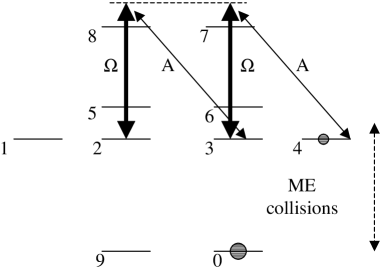
Figure 2: a) Metastable and excited sublevels of ³He. Three coupling constants to the light are introduced. b) Squeezing transfer scheme using a control field $\Omega$, a squeezed vacuum field $A$ and metastability exchange collisions. $9$ and $0$ are the ground state sublevels.

Linearizing the equations in the rotating frame around the fully polarized state solution we obtain the following closed set of equations:

$$\dot{S}_{21} = -(\gamma_{m}-i\delta_{12})S_{21}+i\Omega S_{81}+f_{21}$$ (25)

$$\dot{S}_{81} = -(\gamma-i(\Delta_{18}-2\delta_{las}))S_{81}+i\Omega S_{21}+f_{81}$$ (26)

$$\dot{S}_{32} = \frac{2}{9}\gamma_{m}\left(-\frac{7}{2}S_{32}+\sqrt{3}S_{21}+S_{65}\right)+i\delta_{23}S_{32}-i\Omega(S_{38}-S_{72})+f_{32}$$ (27)

$$\dot{S}_{72} = -(\gamma-i(\Delta_{27}-2\delta_{las}))S_{72}-i\Omega(S_{78}-S_{32})+f_{72}$$ (28)

$$\dot{S}_{43} = \gamma_{m}\left(-\frac{1}{3}S_{43}+\frac{2\sqrt{3}}{9}(S_{32}+S_{65})\right)+\frac{\sqrt{3}}{3}\gamma_{f}I_{09}+i\delta_{34}S_{43}-i\Omega S_{47}+f_{43}$$ (29)

$$\dot{S}_{65} = -\frac{7}{9}\gamma_{m}\left(S_{65}-\frac{2}{7}\sqrt{3}S_{21}-\frac{2}{7}S_{32}\right)+i\delta_{56}S_{65}+f_{65}$$ (30)

$$\dot{S}_{47} = -(\gamma+i\Delta_{47})S_{47}-ig_{A}nA-i\Omega S_{43}+f_{47}$$ (31)

$$\dot{S}_{38} = -(\gamma+i\Delta_{38})S_{38}-i\Omega(S_{32}-S_{78})+f_{38}$$ (32)

$$\dot{S}_{78} = -(2\gamma-i\delta_{87})S_{78}-i\Omega(S_{72}-S_{38})+f_{78}$$ (33)

$$\dot{I}_{09} = \frac{1}{3}\left[-3\gamma_{f}I_{09}+2\gamma_{m}\left(S_{32}-\frac{1}{2}S_{65}+\frac{\sqrt{3}}{2}S_{43}+\frac{\sqrt{3}}{2}S_{21}\right)\right]+i\delta_{90}{I}_{09}+f_{09}$$ (34)

$$\dot{A} = -(\kappa+i\Delta_{C})A-ig_{B}S_{38}-ig_{A}S_{47}+\sqrt{2\kappa}A_{in}$$ (35)

where

$$\Delta_{ij} = (E_{j}-E_{i})-\omega_{2}$$ (36)

$$\delta_{ij} = (E_{j}-E_{i})-\delta_{las}$$ (37)

$$\delta_{las} = \omega_{1}-\omega_{2}\,,$$ (38)

$\gamma$ is the coherence decay rate due to spontaneous emission from the excited state and collisions and we supposed $\Omega$ to be real. The non-zero atomic diffusion coefficients are

$$D_{43,34}=\frac{2}{3}\gamma_{m}n,\hskip 5.69046ptD_{43,90}=D_{09,34}=-\frac{2\sqrt{3}}{3}\gamma_{m}n,\hskip 5.69046ptD_{47,74}=2\gamma n,\hskip 5.69046ptD_{09,09}=2\gamma_{m}n$$ (39)

We notice that metastable variables $S_{21}$, $S_{81}$, $S_{32}$, $S_{72}$, $S_{65}$, $S_{38}$ and $S_{78}$ form a closed subset of equations involving Langevin forces which do not give rise to non-zero diffusion coefficients in the fully polarized limit we consider here. Using the same argument as in section II, we deduce that these variables do not contribute to the spin noise and can be neglected. One is then left with only four relevant equations

$$\dot{S}_{43} = -\frac{\gamma_{m}}{3}S_{43}+\frac{\sqrt{3}}{3}\gamma_{f}I_{09}+i\delta_{34}S_{43}-i\Omega S_{47}+f_{43}$$ (40)

$$\dot{S}_{47} = -(\gamma+i\Delta)S_{47}-ig_{A}nA-i\Omega S_{43}+f_{47}$$ (41)

$$\dot{I}_{09} = \frac{1}{3}\left(-3\gamma_{f}I_{09}+\gamma_{m}\sqrt{3}S_{43}\right)+i\delta_{I}{I}_{09}+f_{09}$$ (42)

$$\dot{A} = -(\kappa+i\Delta_{C})A-ig_{A}S_{47}+\sqrt{2\kappa}A_{in}$$ (43)

with $\Delta=\Delta_{47}$ and $\delta_{I}=\delta_{90}$.

IV Numerical results

Equations (40)-(43) can be used to find the variances of the metastable and ground state spin numerically. A typical result is displayed in figure 3, for which we assume that a squeezed vacuum field with $\Delta X_{in}^{2}=0.5$ is injected into the cavity with the coherent control field in the squeezing-transfer configuration.

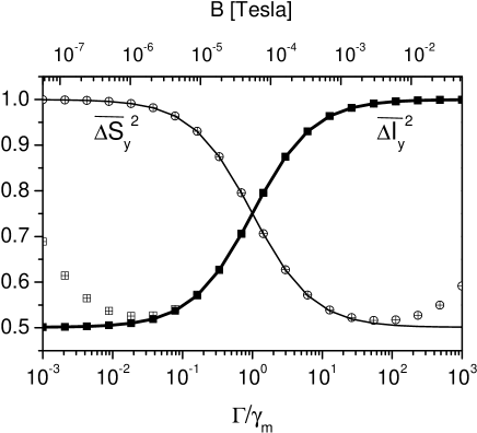
Figure 3: Symbols: numerical calculations for spin variances in ground state (squares) and metastable state (circles), as a function of the ratio $\Gamma/\gamma_{m}$ (lower $x$-axis). The corresponding magnetic field needed to satisfy the resonance conditions (46) and (47) is shown in the upper $x$-axis. Numerical values of parameters are $e^{-2r}=0.5$, $C=500$, $\kappa=100\gamma$, $\Delta=-2000\gamma$, $\gamma=2\times 10^{7}$ s^-1, $\gamma_{m}=5\times 10^{6}$ s^-1. The crossed squares correspond to a calculation including an extra relaxation rate $\gamma_{0}=10^{3}$ s^-1 for the metastable variables. The lines correspond to the analytical predictions (50) and (51).

In this figure $\overline{\Delta{S}_{y}^{2}}$ and $\overline{\Delta I_{y}^{2}}$ represent the variances of $S_{y}$ and $I_{y}$, both normalized to their coherent spin state values. They are plotted as a function of the ratio $\Gamma/\gamma_{m}$, where $\Gamma$ is the pumping parameter

$$\Gamma=\gamma{3\Omega}^{2}(1+C)/\Delta^{2}\,,$$ (44)

and $C=g^{2}n/(\kappa\gamma)$ the cooperativity. It is precisely this ratio $\Gamma/\gamma_{m}$ which acts as a control parameter to decide how the available squeezing of the field is shared between the metastable and the ground state spin. If $\Gamma\gg\gamma_{m}$, correlations are established among the metastable-state spins, the leakage of correlation towards the ground state being negligible. The metastable collective spin is squeezed while the ground state spin remains unsqueezed. In the opposite limit $\Gamma\ll\gamma_{m}$, spin exchange is the dominant process for metastable atoms; they transfer their correlations to the ground state which then becomes squeezed, while the metastable state remains unsqueezed.

In this plot we have chosen the best conditions for squeezing transfer:

1. The metastable coherence $S_{43}$ is resonantly excited by the two fields in a Raman configuration. By introducing the effective two-photon detuning for this coherence

   $$\tilde{\delta}=\delta_{34}+\Omega^{2}/\Delta$$ (45)

   accounting for the light-shift of level 3, this condition reads $\tilde{\delta}=0$, or

   $$(E_{4}-E_{3})/\hbar+\Omega^{2}/\Delta=\omega_{1}-\omega_{2}\,.$$ (46)

2. The ground state coherence $I_{09}$ should be resonantly excited by the metastable coherence ($\delta_{I}=0$), i.e.

   $$(E_{0}-E_{9})/\hbar=\omega_{1}-\omega_{2}\,\,.$$ (47)

In practice a magnetic field (shown as the upper $x$-axis) can be used to simultaneously fulfill (46) and (47). When the resonance conditions are fulfilled the difference in the Larmor frequencies in the metastable and in the ground state is exactly compensated by the light-shift induced by the coherent control field. Choosing $\Gamma=0.1\gamma_{m}$ as a working point, the required field is about $B=57$ mG, corresponding to $\omega_{I}=184$ Hz.

The vapor parameters in the figure correspond to a 1 torr sample at 300 K, with $\gamma_{m}=5\times 10^{6}$ s^-1 and $\gamma=2\times 10^{7}$ s^-1, and a metastable atom density of $3.2\times 10^{10}$ atoms/cm³ which gives $n/N=10^{-6}$. The symbols with a cross are a second calculation in which we added a finite relaxation rate in the metastable state $\gamma_{0}$, to account for the fact that metastable atoms are destroyed as they reach the cell walls. We notice that only the ground state spin squeezing in the region $\Gamma\ll\gamma_{m}$ is affected.

V Analytical results

In order to have a better physical insight it is possible to find simple analytical results within some reasonable approximation. By adiabatic elimination of the polarization $S_{47}$ and the cavity field assuming $\gamma,\kappa\gg\gamma_{m},\gamma_{f}$, one obtains

$$\dot{{S}}_{43}+(\frac{\gamma_{m}}{3}+\frac{\Gamma}{3}-i\tilde{\delta}){S}_{43} = \frac{\gamma_{f}}{\sqrt{3}}{I}_{09}+f_{43}-\frac{\Omega}{\Delta}f_{47}+i\frac{\Omega gn}{\Delta}\sqrt{\frac{2}{\kappa}}A_{in}$$ (48)

$$\dot{{I}}_{09}+(\gamma_{f}-i\delta_{I}){I}_{09} = \frac{\gamma_{m}}{\sqrt{3}}{S}_{43}+f_{09}$$ (49)

In deriving (48) we assumed a Raman configuration $\Delta\gg\gamma$, $\frac{C\gamma}{\Delta}\ll 1$ and that the cavity detuning exactly compensates the cavity field dephasing due to the atoms: $\Delta_{C}=C\kappa\gamma/\Delta$. From equation (48) we see that $(\gamma_{m}+\Gamma)/3$ is the inverse of the characteristic time constant for the metastable coherence evolution.

V.1 Resonant case

If the resonance conditions (46) and (47) are satisfied ($\tilde{\delta}=\delta_{I}=0$) and in the limit $\gamma_{f}\ll\Gamma,\gamma_{m}$, we can calculate the variances of the metastable and ground state spins

$$\Delta I_{y}^{2} = \frac{N}{4}\left\{1-\frac{\gamma_{m}}{\Gamma+\gamma_{m}}\frac{C}{C+1}(1-e^{-2r})\right\}$$ (50)

$$\Delta S_{y}^{2} = \frac{n}{4}\left\{1-\frac{\Gamma}{\Gamma+\gamma_{m}}\frac{C}{C+1}(1-e^{-2r})\right\}$$ (51)

which are plotted as full lines in figure 3.

V.2 Non-perfectly resonant case

In order to test the robustness of our scheme, let us now concentrate on what happens if the resonance conditions (46) and (47) are only approximatively satisfied. We will focus on the variance of the ground state spin coherence $I_{09}$.

By adiabatically eliminating the metastable coherence $S_{43}$ one obtains

$$\dot{{I}}_{09}+\left[\Gamma_{F}+ib\right]{I}_{09}=f_{09}+\frac{\gamma_{m}\sqrt{3}}{\gamma_{m}+\Gamma-i3\tilde{\delta}}\left(f_{43}-\frac{\Omega}{\Delta}f_{47}+i\frac{\Omega gn}{\Delta}\sqrt{\frac{2}{\kappa}}A_{in}\right)$$ (52)

The real part in the brackets

$$\Gamma_{F}=\gamma_{f}\frac{\Gamma(\gamma_{m}+\Gamma)+(3\tilde{\delta})^{2}}{(\gamma_{m}+\Gamma)^{2}+(3\tilde{\delta})^{2}}$$ (53)

is the inverse of the effective time constant for the ground state coherence evolution which would also be the “writing” (or “reading”) time of the quantum memory. $\Gamma_{F}^{-1}=2s$ in the example of figure 3 for $\Gamma=0.1\gamma_{m}$. It would be proportionally shortened by increasing the metastable atoms density although Penning collisions prevent in practice metastable atoms densities exceeding $10^{10}$-$10^{11}$ at/cm². The imaginary part in the brackets

$$b=-\left(\gamma_{f}\frac{3\tilde{\delta}\gamma_{m}}{(\gamma_{m}+\Gamma)^{2}+(3\tilde{\delta})^{2}}+\delta_{I}\right)$$ (54)

is a light-shift “brought back” to the ground state, which is zero in the resonant case. Equation (52) can be used to calculate the best squeezing (optimized with respect to the transverse spin quadrature) of the ground state coherence: $\Delta I_{best}^{2}=\min_{\theta}\Delta I_{\theta}^{2}$ with $I_{\theta}=I_{x}\cos\theta+I_{y}\sin\theta$. We obtain

$$\Delta I_{best}^{2}=\frac{N}{4}\left\{1-\frac{\gamma_{m}}{\Gamma+\gamma_{m}+(3\tilde{\delta})^{2}/\Gamma}\>\frac{C}{C+1}\,\left[1-(e^{-2r}+m\sinh(2r))\right]\right\}$$ (55)

where

$$m=1-\sqrt{\frac{1}{1+(b/\Gamma_{F})^{2}}}$$ (56)

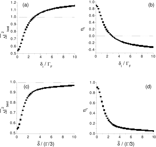
Figure 4: Normalized ground state spin variance corresponding quantum transfer efficiency $\eta_{I}$ as a function of $\delta_{I}/\Gamma_{F}$ (while $\tilde{\delta}=0)$ (plots (a) and (b)), or $\tilde{\delta}/(\Gamma/3)$ (while $\delta_{I}=0)$ (plots (c) and (d). Symbols: numerical integration of equations (25)-(35). Lines: analytical expression (55). Parameters are the same as in figure 3 and $\Gamma=0.1\gamma_{m}$.

We show in figure 4 the effect of a frequency mismatch in on the normalized spin variance, $\overline{\Delta{I}_{y}^{2}}$ and the corresponding squeezing transfer efficiency $\eta_{I}$

$$\eta_{I}=\frac{1-\overline{\Delta{I}_{y}^{2}}}{1-e^{-2r}}\,.$$ (57)

In this example, a frequency mismatch of the order of $\Gamma/3$ in the metastable state or of the order of $\Gamma_{F}$ in the ground state affects the efficiency of the squeezing transfer. The condition for the ground state frequency matching (47) imposes stringent requirements on the homogeneity of the magnetic field. Because of the $\sinh(2r)$ in equation (55), the larger the squeezing the worse are the consequences of a mismatch in the condition on $\delta_{I}=0$ on the ground state atoms. Physically, if a significant dephasing between the squeezed field and the ground state coherence builds up during the squeezing transfer time, the atoms will see an average between the squeezed and the anti-squeezed quadrature of the field noise. We can easily estimate the required magnetic field homogeneity as follows. Let us introduce the Larmor evolution frequencies in the metastable and ground states: in low field, $\hbar\omega_{\alpha}=\mu_{\alpha}B$ ($\alpha$=I,S) with $\mu_{I}/h=3.24$kHz/G and $\mu_{S}/h=1.87$MHz/G, and let $\Delta B$ be the maximum field difference with respect to the optimal value in the cell volume. For low field, the condition on $\Delta B$ to preserve the transfer efficiency reads $\mu_{I}\Delta B\ll h\Gamma_{F}$. Since $\Omega^{2}/\Delta\simeq\Gamma\frac{\Delta}{3\gamma C}\simeq\frac{\mu_{S}}{h}B$ we get $\frac{\Gamma}{\Gamma_{F}}\frac{\mu_{I}}{\mu_{S}}\frac{\Delta}{3\gamma C}\frac{\Delta B}{B}<1$ or, in the regime $\Gamma\ll\gamma_{m}$, $600\frac{\Delta}{\gamma C}\frac{\Delta B}{B}\ll 1$. With the parameters of figure 3 this gives a condition on the magnetic field inhomogeneity: $\Delta B/B\ll 4\times 10^{-4}$. In figure 5 we calculated the variance of the ground state spin as a function of $\Gamma/\gamma_{m}$ for an increasing inhomogeneity $\Delta B/B$ from zero (thick line) to $6\times 10^{-4}$. In practice a homogeneity of 100 ppm should be sufficient for the chosen parameters to guarantee that all atoms will be squeezed.

Figure 5: Normalized “best” variance of the ground state spin as a function of $\Gamma/\gamma_{m}$ (lower $x$-axis) for an increasing inhomogeneity $\Delta B/B$ from zero to $6\times 10^{-4}$ by steps of $1\times 10^{-4}$. On the upper $x$-axis we show the corresponding homogeneous magnetic field needed to satisfy resonance conditions (46) and (47). Numerical values of parameters are $e^{-2r}=0.5$, $C=500$, $\kappa=100\gamma$, $\Delta=-2000\gamma$, $\gamma=2\times 10^{7}$ s^-1, $\gamma_{m}=5\times 10^{6}$ s^-1, $\gamma_{0}=0$.

VI Optical readout

VI.1 Outgoing field squeezing

As briefly stressed in prl the squeezed fluctuations which are stored into the nuclear spins can be retrieved optically in the field exiting the cavity by using the reverse transfer process. Indeed, once the write sequence of the quantum memory has been completed, both the fields and the discharge can be switched off, leaving the atoms in the fundamental state in a spin-squeezed state. After a variable storage time, switching back on the discharge and only the control field in the same configuration as for the writing phase ($\Gamma\ll\gamma_{m}$), will rapidly put a small fraction of atoms in the metastable state and start the reverse transfer process from the fundamental atoms to the field. The correlations in the ground state will slowly transfer via the metastable state to the intracavity field. This will then result in squeezed fluctuations for the field exiting the cavity, which can be measured by homodyne detection.

More quantitatively, if we still assume that the metastable spin observables and the intra-cavity field adiabatically follow the ground state spin observables and the evolution equations for the fluctuations of the squeezed component are in the resonant situation, we have

$$\dot{I}_{y}(t) = -\Gamma_{F}I_{y}(t)+\beta X_{in}(t)+\tilde{f}_{y}(t)$$ (58)

$$X_{out}(t) = \sqrt{2\kappa}X(t)-X_{in}(t)$$ (59)

with

$$\beta = \frac{\gamma_{m}}{\gamma_{m}+\Gamma}\frac{g_{A}n\Omega\sqrt{3}}{2\Delta}\sqrt{\frac{2}{\kappa}}$$ (60)

$$\tilde{f}_{y} = \frac{\gamma_{m}\sqrt{3}}{\gamma_{m}+\Gamma}\left[\frac{f_{43}-f_{34}}{2i}-\frac{\Omega}{\Delta}\frac{f_{74}-f_{47}}{2i}\right]+\frac{f_{09}-f_{90}}{2i}$$ (61)

Denoting by $t=0$ the start of the readout sequence and by $e^{-2r}=\Delta I_{y}^{2}(0)/(N/4)$ the initial squeezing of the ground state nuclear spin, the two-time correlation function of the outgoing field amplitude quadrature can be obtained via (59) after integration of (58)

$$\mathcal{C}(t,t^{\prime})\equiv\langle X^{out}(t)X^{out}(t^{\prime})\rangle=\delta(t-t^{\prime})-2\Gamma_{F}\eta_{I}[1-e^{-2r}]e^{-\Gamma_{F}(t+t^{\prime})}$$ (62)

The $\delta$-correlated term corresponds to the vacuum fluctuations contribution, whereas the second term corresponds to a transient squeezing for the outgoing field which is proportional to the initial atomic squeezing. In (62), $\eta_{I}$ designates the optimal quantum transfer efficiency in the ground state

$$\eta_{I}=\frac{\gamma_{m}}{\gamma_{m}+\Gamma}\frac{C}{C+1}$$ (63)

The ground state squeezing can be adequately measured by homodyne detection using a temporally matched local oscillator as shown in Refs. dantanpra04 ; dantanpulse . Using a local oscillator with envelope $\mathcal{E}(t)$ the normalized power measured by a Fourier-limited spectrum analyzer integrating over a time $T$ is given by

$$P(t) = \frac{1}{\mathcal{E}(t)^{2}}\int_{-\pi/T}^{\pi/T}\frac{d\omega}{2\pi}\int_{t}^{t+T}d\tau\int_{t}^{t+T}d\tau^{\prime}e^{-i\omega(\tau-\tau^{\prime})}\mathcal{E}(\tau)\mathcal{E}(\tau^{\prime})\mathcal{C}(\tau,\tau^{\prime})$$ (64)

In order to measure the atomic squeezing one has to maximize the temporal overlap between the local oscillator and the field radiated by the atoms: $\mathcal{E}(t)\propto e^{-\Gamma_{F}t}$. For such a local oscillator and for an integration time longer than the readout time $\Gamma_{F}^{-1}$ the measured power can be written as the sum of a shot-noise term $\mathcal{N}$ and a time-dependent signal term $\mathcal{S}$ proportional to the initial squeezing:

$$P(t)=\mathcal{N}-\mathcal{S}[1-e^{-2r}]e^{-2\Gamma_{F}t}$$ (65)

with $\mathcal{S}\simeq\eta_{I}\mathcal{N}$. The ground state nuclear spin fluctuations can therefore be measured optically with the same efficiency $\eta_{I}$ as in the write sequence. However, because of the slow character of the correlation transfer process in the ground state the readout time is as long as the write time. As expected it is not possible to access the quantum memory faster during the readout than during the write phase. One could think of a faster readout method by transferring the fundamental atoms fluctuations to the metastable atoms and perform the optical readout in the regime $\Gamma\gg\gamma_{m}$. However, as we showed in section II, starting with a squeezed fundamental spin and first switching on the discharge (without the fields) will transfer very few correlations from the fundamental to the metastable atoms and almost no squeezing will be retrieved in the field.

VII Entangling two separate samples

A direct and important extension of the previous results is that it is possible to transfer quantum correlations between different light beams to two spatially separated nuclear spins. If one disposes of EPR fields this allows to entangle two separate ensembles dantanEPL04 . Such EPR atomic states are very useful for quantum information protocols involving the manipulation of continuous variable entanglement, such as atomic teleportation for instance dantanprl05 .

Let us consider two identical ensembles 1 and 2 illuminated by EPR-correlated vacuum fields $A^{(i)}_{in}$ and coherent control fields $\Omega_{i}$ ($i=1,2$). Without loss of generality we assume symmetrical field correlations of the form

$$\Delta^{2}X^{(i)}_{in} = \Delta^{2}Y^{(i)}_{in}=\cosh(2r)\hskip 8.5359pt(i=1,2)$$ (66)

$$\langle X^{(i)}_{in}X^{(j)}_{in}\rangle = -\langle Y^{(i)}_{in}Y^{(j)}_{in}\rangle=\sinh(2r)\hskip 8.5359pt(i\neq j),$$ (67)

i.e. that the amplitude quadratures are correlated and the phase quadratures anti-correlated: $\Delta^{2}(X^{(1)}_{in}-X^{(2)}_{in})=\Delta^{2}(Y^{(1)}_{in}+Y^{(2)}_{in})=2e^{-2r}$. For perfect entanglement ($r=\infty$) these EPR variances vanish. Both spins are initially prepared in a coherent spin state and we assume an equal incident power on both samples ($\Omega_{1}=\Omega_{2}$). Under the same adiabatic approximations as before, the fluctuations of the transverse spin components satisfy equation of the form (58)

$$\dot{I}_{xi} = -\Gamma_{F}I_{xi}-\beta Y^{(i)}_{in}+\tilde{f}_{xi},$$ (68)

$$\dot{I}_{yi} = -\Gamma_{F}I_{yi}+\beta X^{(i)}_{in}+\tilde{f}_{yi},$$ (69)

($i=1,2$). Because of the linearity of the coupling in this regime, the EPR atomic nuclear spin operators, $I_{x1}+I_{x2}$ and $I_{y1}-I_{y2}$, are clearly coupled to the EPR field operators

$$\frac{d}{dt}(I_{x1}+I_{x2}) = -\Gamma_{F}(I_{x1}+I_{x2})-\beta(Y^{(1)}_{in}+Y^{(2)}_{in})+\tilde{f}_{x1}+\tilde{f}_{x2}$$ (70)

$$\frac{d}{dt}(I_{y1}-I_{y2}) = -\Gamma_{F}(I_{y1}-I_{y2})+\beta(X^{(1)}_{in}-X^{(2)}_{in})+\tilde{f}_{y1}-\tilde{f}_{y2}$$ (71)

The amount of EPR-type correlations between the incident fields is given by the half-sum of the EPR variances

$$\mathcal{E}_{f}=\frac{1}{2}\left[\Delta^{2}(X^{(1)}_{in}-X^{(2)}_{in})+\Delta^{2}(Y^{(1)}_{in}+Y^{(2)}_{in})\right]=2e^{-2r}$$ (72)

In the Gaussian approximation the entanglement between the nuclear spins can be evaluated using the same quantity (also normalized to 2)

$$\mathcal{E}_{I}=\frac{2}{N}\left[\Delta^{2}(I_{x1}+I_{x2})+\Delta^{2}(I_{y1}-I_{y2})\right]$$ (73)

It follows from (70-71) that the last two quantities are simply related by

$$\mathcal{E}_{I}=\eta_{I}\mathcal{E}_{f}+2(1-\eta_{I}).$$ (74)

Like squeezing entanglement can also be in principle perfectly mapped onto the nuclear spins with an efficiency $\eta_{I}$ (63), close to unity in the regime $\Gamma\gg\gamma_{m}$ and $C\gg 1$. Let us introduce the correlation functions $\mathcal{C}_{I}^{(i,i)}$ of individual spins inside the ensemble $i$ (i=1,2):

$$\mathcal{C}_{I}^{(i,i)}=\frac{\overline{\Delta I_{xi}^{2}}-1}{4N}\hskip 28.45274pt(i=1,2)$$ (75)

and the correlation function $\mathcal{C}_{I}^{(i,j)}$ of two individual spins belonging to the different ensembles $i$ and $j$:

$$\mathcal{C}_{I}^{(i,j)}=\frac{\overline{\langle I_{xi}I_{xj}\rangle}}{4N}\hskip 28.45274pt(i\neq j=1,2)$$ (76)

where the overline indicates the normalization of the correlation functions to $N/4$. In our case for $\eta_{I}\simeq 1$ we get:

$$\mathcal{C}_{I}^{(1,1)} = \mathcal{C}_{I}^{(2,2)}\simeq\frac{\cosh(2r)-1}{4N}$$ (77)

$$\mathcal{C}_{I}^{(1,2)} = \mathcal{C}_{I}^{(2,1)}\simeq\frac{\sinh(2r)}{4N}\,.$$ (78)

It is interesting to note that the two correlation functions $\mathcal{C}_{I}^{(1,1)}$ and $\mathcal{C}_{I}^{(1,2)}$ become approximately equal for a large entanglement $e^{2r}\gg 1$ so that an individual spin is about as much correlated with the other spins in its own ensemble as with the spins of the other ensemble.

VIII The imperfect polarization case

The nuclear polarization of the sample is defined as

$$P=\frac{\langle I_{00}\rangle-\langle I_{99}\rangle}{\langle I_{00}\rangle+\langle I_{99}\rangle}$$ (79)

In practice polarization between 80% and 85% are currently achieved by optical pumping in dilute ³He samples nacher85 . If the atoms are prepared in a state which is not fully polarized - $P\neq 1$ - the situation is clearly more complicated than we described in prl and in the present paper. In particular, equations (25)-(35) and (39) obtained by linearization around the fully polarized state are no longer valid. We did not perform a complete analysis in the $P\neq 1$ case. However, one can have a good idea of the result by using the simplified model of prl which involves only two metastable sublevels (see figure 6). As in section III, a Raman transition is driven by a coherent control field of Rabi frequency $\Omega$ and a squeezed vacuum cavity field:

$$H=H_{0}+\hbar\left\{\Omega\,\tilde{S}_{31}e^{-i\omega_{1}t}+g\,A\,\tilde{S}_{32}+\rm{h.c.}\right\}\,.$$ (80)

In this toy-model the control field $\Omega$ also acts as an optical pumping beam (able to transfer the atoms from sublevel $9$ to sublevel $0$) and we introduce explicitly a relaxation in the ground state, so that $P\neq 1$ in steady state.

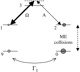
Figure 6: Sublevels $1$ and $2$ are metastable, level $3$ is the excited state, $9$ and $0$ are the ground state sublevels. We include a relaxation process in the ground state so that $P\neq 1$ in steady state.

Let us introduce for this model the rescaled coupling constant $\tilde{g}$, the atomic one-photon detunings $\Delta_{1}$ and $\Delta$, the two-photon detunings $\tilde{\delta}$ and $\delta_{I}$, and two pumping parameters $\Gamma_{p}$ and $\Gamma$:

$$\Delta_{1} = (E_{3}-E_{1})/\hbar-\omega_{1},\hskip 28.45274pt\Delta=(E_{3}-E_{2})/\hbar-\omega_{2},$$ (81)

$$\tilde{\delta} = \Delta_{1}-\Delta+\frac{\Omega^{2}}{\Delta},\hskip 56.9055pt\delta_{I}=(E_{0}-E_{9})/\hbar-(\omega_{1}-\omega_{2}),$$ (82)

$$\Gamma_{P} = \gamma\frac{\Omega^{2}}{\Delta^{2}},\hskip 99.58464pt\Gamma=\Gamma_{p}(1+C),$$ (83)

where $\gamma$ is the optical coherence decay rate and $C$ is the cooperativity parameter defined by equation (44). For the atomic operators we introduce $\tilde{S}_{+}=\tilde{S}_{21}$, $\tilde{S}_{-}=\tilde{S}_{12}$

$$\tilde{S}_{x}=(\tilde{S}_{-}+\tilde{S}_{+})/2,\hskip 28.45274pt\tilde{S}_{y}=i(\tilde{S}_{-}-\tilde{S}_{+})/2,\hskip 28.45274pt\tilde{S}_{z}=(\tilde{S}_{22}-\tilde{S}_{11})/2,\hskip 28.45274pt$$ (84)

and similarly for the ground state operators. In the limit of large one photon detunings the excited state and the optical coherences can be adiabatically eliminated, yielding a set of equations similar to those of Ref. dantanPRA03 with the addition of metastability exchange. By adiabatically eliminating the field (assumed to be resonant in the cavity) and for $\tilde{\delta}=0$, $\delta_{I}=0$, we obtain:

$$\dot{\tilde{S}}_{+} = -(\Gamma_{p}+\gamma_{m})\tilde{S}_{+}+\gamma_{f}I_{+}+2i\tilde{g}A\tilde{S}_{z}++f_{\tilde{S}_{+}}$$ (85)

$$\dot{\tilde{S}}_{z} = -(\Gamma_{p}+\gamma_{m})\tilde{S}_{z}+\gamma_{f}I_{z}+\frac{n\Gamma_{p}}{2}+i\tilde{g}[A^{\dagger}\tilde{S}_{+}-A\tilde{S}_{-}]+f_{\tilde{S}_{z}}$$ (86)

$$\dot{A} = -(\kappa+i\Delta_{C})A+i\tilde{g}\tilde{S}_{+}+\sqrt{2\kappa}A_{in}$$ (87)

$$\dot{I}_{+} = -(\gamma_{f}+\Gamma_{1})I_{+}+\gamma_{m}\tilde{S}_{+}+f_{I_{+}}$$ (88)

$$\dot{I}_{z} = -(\gamma_{f}+\Gamma_{1})I_{z}+\gamma_{m}\tilde{S}_{z}+f_{I_{z}}$$ (89)

The semiclassical version of equations (85)-(89) has a stationary solution $\langle\tilde{S}_{+}\rangle=\langle I_{+}\rangle=\langle A_{in}\rangle=0$ and with

$$\langle\tilde{S}_{z}\rangle = \frac{\gamma_{f}+\Gamma_{1}}{\gamma_{m}}\langle I_{z}\rangle\hskip 56.9055ptP=\frac{1}{1+\Gamma_{1}(\Gamma_{p}+\gamma_{m})/(\Gamma_{p}\gamma_{f})}$$ (90)

We will have in practice $\Gamma_{1}\ll\gamma_{f}$, meaning that the nuclear polarization in the metastable state $P^{\ast}=\langle\tilde{S}_{z}\rangle/(n/2)$ and the nuclear polarization in the ground state $P=\langle I_{z}\rangle/(N/2)$ are almost equal. In this toy-model the stationary $P$ is determined by the balance between the decay $\Gamma_{1}$ and the pumping $\Gamma_{p}$. In reality, the atoms will be previously pumped more efficiently with resonant light. When we linearize the equations around the steady state we obtain

$$\dot{\tilde{S}}_{+} = -(\tilde{\Gamma}+\gamma_{m})\tilde{S}_{+}+\frac{ig\Omega n}{\kappa\Delta}P^{\ast}\sqrt{2\kappa}A_{in}+\gamma_{f}I_{+}+f_{\tilde{S}_{+}}$$ (91)

$$\dot{I}_{+} = -(\gamma_{f}+\Gamma_{1})I_{+}+\gamma_{m}\tilde{S}_{+}+f_{I_{+}}$$ (92)

with

$$\tilde{\Gamma}=\Gamma_{p}(1+CP^{\ast})$$ (93)

Starting from equations (91)-(92) one can proceed as in section V to obtain

$$\overline{\Delta{I}_{y}^{2}}=\frac{\Delta I_{y}^{2}}{NP/4}=\frac{1}{P}+(P^{*}e^{-2r}-1)\eta_{I}^{\prime}+\frac{\eta_{I}^{\prime}}{2\tilde{C}}\frac{P^{*}-1}{P}$$ (94)

where

$$\tilde{C} = CP^{\ast}\hskip 28.45274pt\textrm{and}\hskip 28.45274pt\tilde{\Gamma}_{f}=\frac{\gamma_{f}\tilde{\Gamma}}{\tilde{\Gamma}+\gamma_{m}}$$ (95)

$$\eta_{I}^{\prime} = \frac{\tilde{C}}{\tilde{C}+1}\;\frac{\gamma_{m}}{\tilde{\Gamma}+\gamma_{m}}\;\frac{\tilde{\Gamma}_{f}}{\tilde{\Gamma}_{f}+\Gamma_{1}}$$ (96)

For $P^{\ast}\simeq P$ and $\tilde{C}\gg 1$, we have finally

$$\overline{\Delta{I}_{y}^{2}}=\eta_{I}^{\prime}e^{-2r}+(1-\eta_{I}^{\prime})/P$$ (97)

Equation (97) shows that the main consequence of having $P\neq 1$ is a rescaling of the cooperativity and the pumping parameter $\tilde{\Gamma}$ and the quantum transfer efficiency $\eta_{I}^{\prime}$, which are reduced by a factor $P$. Let us note that, for $P\neq 1$, when no squeezing enters the cavity, the atoms are no longer in a coherent spin state. This shows, however, that strong squeezing transfer is still possible with a non-ideal polarization.

IX Appendix

Evolution equations of the density matrix elements under ME collisions are:

$${\frac{d}{dt}}\rho_{{11}}= \gamma_{{{\rm exc}}} \left(-N\rho_{{11}}+\frac{1}{3}\rho_{{99}}\left(\rho_{{22}}+3\rho_{{11}}+2\rho_{{55}}\right)\right)\$$

$${\frac{d}{dt}}\rho_{{12}}= \gamma_{{{\rm exc}}} \left(-N\rho_{{12}}+\frac{2}{9}\rho_{{99}}\left(\left(\rho_{{23}}+\rho_{{56}}\right)\sqrt{3}+3\rho_{{12}}\right)+\frac{\sqrt{3}}{9}\rho_{{90}}\left(\rho_{{22}}+3\rho_{{11}}+2\rho_{{55}}\right)\right)\$$

$${\frac{d}{dt}}\rho_{{13}}= \gamma_{{{\rm exc}}} \left(-N\rho_{{13}}+\frac{1}{3}\rho_{{99}}\left(\rho_{{13}}+\rho_{{24}}\right)+\frac{2}{9}\rho_{{90}}\left(\left(\rho_{{23}}+\rho_{{56}}\right)\sqrt{3}+3\rho_{{12}}\right)\right)\$$

$${\frac{d}{dt}}\rho_{{14}}= \gamma_{{{\rm exc}}} \left(-N\rho_{{14}}+\frac{\sqrt{3}}{3}\rho_{{90}}\left(\rho_{{13}}+\rho_{{24}}\right)\right)\$$

$${\frac{d}{dt}}\rho_{{22}}= \gamma_{{{\rm exc}}} \left(-N\rho_{{22}}+\frac{2}{9}\rho_{{99}}\left(2\rho_{{22}}+\rho_{{55}}+\rho_{{66}}+2\rho_{{33}}\right)+\frac{2}{9}\rho_{{90}}\left(\sqrt{3}\rho_{{21}}+\rho_{{65}}+\rho_{{32}}\right)\right.\$$

$$\,\,\,\,\left.+\frac{2}{9}\rho_{{09}}\left(\sqrt{3}\rho_{{12}}+\rho_{{23}}+\rho_{{56}}\right)+\frac{1}{9}\rho_{{00}}\left(\rho_{{22}}+3\rho_{{11}}+2\rho_{{55}}\right)\right)\$$

$${\frac{d}{dt}}\rho_{{23}}= \gamma_{{{\rm exc}}} \left(-N\rho_{{23}}+\frac{2}{9}\rho_{{99}}\left(\sqrt{3}\rho_{{34}}+\rho_{{56}}+\rho_{{23}}\right)+\frac{2}{9}\rho_{{90}}\left(2\rho_{{22}}+\rho_{{55}}+\rho_{{66}}+2\rho_{{33}}\right)\right.\$$

$$\,\,\,\,\left.+\frac{\sqrt{3}}{9}\rho_{{09}}\left(\rho_{{13}}+\rho_{{24}}\right)+\frac{2}{9}\rho_{{00}}\left(\sqrt{3}\rho_{{12}}+\rho_{{23}}+\rho_{{56}}\right)\right)\$$

$${\frac{d}{dt}}\rho_{{24}}= \gamma_{{{\rm exc}}} \left(-N\rho_{{24}}+\frac{2}{9}\rho_{{90}}\left(\sqrt{3}\left(\rho_{{23}}+\rho_{{56}}\right)+3\rho_{{34}}\right)+\frac{1}{3}\rho_{{00}}\left(\rho_{{13}}+\rho_{{24}}\right)\right)\$$

$${\frac{d}{dt}}\rho_{{33}}= \gamma_{{{\rm exc}}} \left(-N\rho_{{33}}+\frac{1}{9}\rho_{{99}}\left(2\rho_{{66}}+\rho_{{33}}+3\rho_{{44}}\right)+\frac{2}{9}\rho_{{90}}\left(\sqrt{3}\rho_{{43}}+\rho_{{65}}+\rho_{{32}}\right)\right.\$$

$$\,\,\,\,\left.+\frac{2}{9}\rho_{{09}}\left(\sqrt{3}\rho_{{34}}+\rho_{{56}}+\rho_{{23}}\right)+\frac{2}{9}\rho_{{00}}\left(2\rho_{{22}}+\rho_{{55}}+\rho_{{66}}+2\rho_{{33}}\right)\right)\$$

$${\frac{d}{dt}}\rho_{{34}}= \gamma_{{{\rm exc}}} \left(-N\rho_{{34}}+\frac{\sqrt{3}}{9}\rho_{{90}}\left(2\rho_{{66}}+\rho_{{33}}+3\rho_{{44}}\right)+\frac{2}{9}\rho_{{00}}\left(\sqrt{3}\left(\rho_{{23}}+\rho_{{56}}\right)+3\rho_{{34}}\right)\right)\$$

$${\frac{d}{dt}}\rho_{{44}}= \gamma_{{{\rm exc}}} \left(-N\rho_{{44}}+\frac{1}{3}\rho_{{00}}\left(2\rho_{{66}}+\rho_{{33}}+3\rho_{{44}}\right)\right)\$$

$${\frac{d}{dt}}\rho_{{55}}= \gamma_{{{\rm exc}}} \left(-N\rho_{{55}}+\frac{1}{9}\rho_{{99}}\left(2\rho_{{22}}+\rho_{{55}}+\rho_{{66}}+2\rho_{{33}}\right)-\frac{2}{9}\rho_{{90}}\left(\sqrt{3}\rho_{{21}}+\rho_{{65}}+\rho_{{32}}\right)\right.\$$

$$\,\,\,\,\left.-\frac{2}{9}\rho_{{09}}\left(\sqrt{3}\rho_{{12}}+\rho_{{23}}+\rho_{{56}}\right)+\frac{2}{9}\rho_{{00}}\left(\rho_{{22}}+3\rho_{{11}}+2\rho_{{55}}\right)\right)\$$

$${\frac{d}{dt}}\rho_{{56}}= \gamma_{{{\rm exc}}} \left(-N\rho_{{56}}+\frac{2}{9}\rho_{{99}}\left(\sqrt{3}\rho_{{34}}+\rho_{{56}}+\rho_{{23}}\right)-\frac{1}{9}\rho_{{90}}\left(2\rho_{{22}}+\rho_{{55}}+\rho_{{66}}+2\rho_{{33}}\right)\right.\$$

$$\,\,\,\,\left.-\frac{2\sqrt{3}}{9}\rho_{{09}}\left(\rho_{{13}}+\rho_{{24}}\right)+\frac{2}{9}\rho_{{00}}\left(\sqrt{3}\rho_{{12}}+\rho_{{23}}+\rho_{{56}}\right)\right)\$$

$${\frac{d}{dt}}\rho_{{66}}= \gamma_{{{\rm exc}}} \left(-N\rho_{{66}}+\frac{2}{9}\rho_{{99}}\left(2\rho_{{66}}+\rho_{{33}}+3\rho_{{44}}\right)-\frac{2}{9}\rho_{{90}}\left(\sqrt{3}\rho_{{43}}+\rho_{{65}}+\rho_{{32}}\right)\right.\$$

$$\,\,\,\,\left.-\frac{2}{9}\rho_{{09}}\left(\sqrt{3}\rho_{{34}}+\rho_{{56}}+\rho_{{23}}\right)+\frac{1}{9}\rho_{{00}}\left(2\rho_{{22}}+\rho_{{55}}+\rho_{{66}}+2\rho_{{33}}\right)\right)\$$

$${\frac{d}{dt}}\rho_{{00}}= \gamma_{{{\rm exc}}} \left(-n\rho_{{00}}+\frac{1}{3}\left(3\rho_{{44}}+\rho_{{66}}+\rho_{{22}}+2\rho_{{55}}+2\rho_{{33}}\right)N\right)\$$

$${\frac{d}{dt}}\rho_{{09}}= \gamma_{{{\rm exc}}} \left(-n\rho_{{09}}+\frac{1}{3}N\left(\left(\rho_{{43}}+\rho_{{21}}\right)\sqrt{3}+2\rho_{{32}}-\rho_{{65}}\right)\right)\$$

$${\frac{d}{dt}}\rho_{{99}}= \gamma_{{{\rm exc}}} \left(-n\rho_{{99}}+\frac{1}{3}\left(\rho_{{33}}+2\rho_{{22}}+3\rho_{{11}}+\rho_{{55}}+2\rho_{{66}}\right)N\right)\$$

References

• (1) W. Heil, H. Humblota, E. Otten, M. Schafera, R. Sarkaua and M. Leduc, Phys. Lett A, 201, 337 (1995)
• (2) C.Cohen-Tannoudji, J. Dupont-Roc, S. Haroche and F. Laloë, Phys. Rev. Lett. 22, 758 (1969)
• (3) A. Dantan, G. Reinaudi, A. Sinatra, F. Laloë, E. Giacobino, M. Pinard, Phys. Rev. Lett. 95, 123002 (2005)
• (4) M. Fleischhauer and M.D. Lukin, Phys. Rev. Lett. 84, 5094 (2000)
• (5) A.E. Kozhekin, K. Mølmer and E. Polzik, Phys. Rev. A 62, 033809 (2000)
• (6) A. Dantan and M. Pinard, Phys. Rev. A 69, 43810 (2004)
• (7) C.H. van der Wal et al., Science 301, 196 (2003)
• (8) C. Schori, B. Julsgaard, J.L. Sørensen, E.S. Polzik, Phys. Rev. Lett. 89, 57903 (2002)
• (9) B. Julsgaard, J. Sherson, J.I. Cirac, J. Fiurášek, E.S. Polzik, Nature (London) 432, 482 (2004)
• (10) B. Julsgaard, A. Khozekin, E.S. Polzik, Nature (London) 413, 400 (2001)
• (11) F.D. Colegrove , L.D. Schearer and G.K. Walters, Phys. Rev. 132, 2561 (1963)
• (12) R.B. Partridge and G.W. Series, Proc. Phys. Soc. 88, 983 (1966)
• (13) J. Becker et al., Nucl. Instrum. Methods Phys. Res. A 402, 327 (1998); H. Moller et al., Magn. Reson. Med. 47, 1029 (2002)
• (14) C. Cohen-Tannoudji, J. Dupont-Roc, G. Grynberg “Atom-Photon Interactions”, Wiley-VCH, Berlin (1998), ch. V.
• (15) In practice one wants the squeezed field and the coherent field to be copropagating. The squeezed field should thus be $\sigma$-polarized, with a $\sigma^{+}$ component; we checked that this component plays no role here.
• (16) A. Dantan, J. Cviklinski, M. Pinard, Ph. Grangier, quant-ph/0512175.
• (17) A. Dantan, M. Pinard, V. Josse, N. Nayak, P.R. Berman, Phys. Rev A 67, 045801 (2003)
• (18) A. Dantan, A. Bramati and M. Pinard, Europhys. Lett. 67, 881 (2004)
• (19) A. Dantan, N. Treps, A. Bramati, M. Pinard, Phys. Rev. Lett. 95, 050520 (2005)
• (20) P.-J. Nacher, M. Leduc, J. Physique 46, 2057 (1985).