Kaonic Qubits

Abstract

Quantum mechanics can also be tested in high energy physics; in particular, the neutral kaon system is very well suited. We show that these massive particles can be considered as qubits —kaonic qubits— in the very same way as spin–$\frac{1}{2}$ particles or polarized photons. But they also have other important properties, namely they are instable particles and they violate the $CP$ symmetry ($C$…charge conjugation, $P$…parity). We consider a Bell inequality and, surprisingly, the premises of local realistic theories require strict $CP$ conservation, in contradiction to experiment. Furthermore we investigate Bohr’s complementary relation in order to describe the physics of the time evolution of kaons. Finally, we discuss quantum marking and eraser experiments with kaons, which prove in a new way the very concept of a quantum eraser.

PACS numbers: 03.65.Ud, 03.65.Ta, 13.25.Es, 11.30.Er
Key-Words: kaons, entanglement, Bell inequality, double slits, quantum eraser

I Introduction

For questioning the peculiarities of quantum theory the systems produced in high energy accelerators are very well suited. The purpose of this Article is to demonstrate various similarities of such massive systems with the usually considered photonic systems as well as the important differences and to show new and different tests of the foundations of quantum mechanics.

We are going to focus here on the neutral kaon system (for an overview see Ref. BertlmannSchladming and references therein). We show that for this system the superposition principle is realized in the very same way as for photons or spin–$\frac{1}{2}$ particles and that also entangled two–kaon states can be produced. The time evolution —kaons oscillate in time and decay— and the violation of $CP$ symmetry ($C$…charge conjugation transforming a particle into its anti–particle, $P$…parity), which means that the world is not mirrored into an antiworld, are very specific for this system.

Surprisingly, a Bell inequality can be established whose violation is connected to the violation of $CP$ symmetry. Here two different concepts meet each other, the concept of local realism and the concept of symmetry which is fundamental in particle physics.

Furthermore, the nature of kaons offers us to study other puzzling aspects of quantum theory, in particular, Bohr’s complementary principle in a double–slit–like scenario and the quantum marking and eraser concepts. For the later there exist experimental setups which are not just analogous to existing quantum eraser experiments but also new ones since the complementary observables can be measured in two different ways, via “active” and “passive” measurements.

II Kaons as qubits

What are K-mesons or simply kaons? They are bound states of quarks and anti-quarks ($q\bar{q}$), where the quark ($q=u,d,s$) can be the up, down, or strange quark, and can be summarized as follows:

$\vphantom{\biggr{\{}}K$-meson	quarks	$S$	$I_{3}$
$K^{+}$	$u\bar{s}$	$+1$	$+1/2$
$K^{-}$	$\bar{u}s$	$-1$	$-1/2$
$K^{0}$	$d\bar{s}$	$+1$	$-1/2$
$\bar{K}^{0}$	$\bar{d}s$	$-1$	$+1/2$
$\;K^{0}$ particle	$\;\bar{K}^{0}$ antiparticle	$\;S$ strangeness	$\;I$ isospin

Not just for particle physicists the neutral kaon system is unique, these strange mesons are also fantastic quantum systems, we could even say they are selected by Nature to demonstrate fundamental quantum principles such as:

• superposition principle

• oscillation and decay property

• quasi-spin property.
  

Their mass is about $497$ MeV and they are pseudoscalars $J^{P}=0^{-}\,$. They interact via strong interactions which are $S$ conserving and weak interactions which are $S$ violating. It is due to the weak interactions that the kaons oscillate $K^{0}\,\longleftrightarrow\,\bar{K}^{0}\,$.

Quantum states of kaons

Quantum–mechanically we can describe the kaons in the following way. Kaons are characterized by their strangeness quantum number $+1,-1$

$$S|K^{0}\rangle=+|K^{0}\rangle\;,\qquad S|\bar{K}^{0}\rangle=-|\bar{K}^{0}\rangle\;,$$ (1)

and the combined operation $CP$ gives

$$CP|K^{0}\rangle=-|\bar{K}^{0}\rangle\;,\qquad CP|\bar{K}^{0}\rangle=-|K^{0}\rangle\;.$$ (2)

It is straightforward to construct the $CP$ eigenstates

$$|K_{1}^{0}\rangle=\frac{1}{\sqrt{2}}\big{\{}|K^{0}\rangle-|\bar{K}^{0}\rangle\big{\}}\;,\qquad|K_{2}^{0}\rangle=\frac{1}{\sqrt{2}}\big{\{}|K^{0}\rangle+|\bar{K}^{0}\rangle\big{\}}\;,$$ (3)

a quantum number conserved in strong interactions

$$CP|K_{1}^{0}\rangle=+|K_{1}^{0}\rangle\;,\qquad CP|K_{2}^{0}\rangle=-|K_{2}^{0}\rangle\;.$$ (4)

However, due to weak interactions $CP$ symmetry is violated and the kaons decay in physical states, the short– and long–lived states, $|K_{S}\rangle,|K_{L}\rangle$, which differ slightly in mass, $\Delta m=m_{L}-m_{S}=3.49\times 10^{-6}$ eV, but immensely in their lifetimes and decay modes

$$|K_{S}\rangle=\frac{1}{N}\big{\{}p|K^{0}\rangle-q|\bar{K}^{0}\rangle\big{\}}\;,\qquad|K_{L}\rangle=\frac{1}{N}\big{\{}p|K^{0}\rangle+q|\bar{K}^{0}\rangle\big{\}}\;.$$ (5)

The weights $p=1+\varepsilon$, $\,q=1-\varepsilon,\,$ with $N^{2}=|p|^{2}+|q|^{2}$ contain the complex $CP$ violating parameter $\varepsilon$ with $\lvert\varepsilon\rvert\approx 10^{-3}$. $CPT$ invariance is assumed ($T\dots$ time reversal). The short–lived K–meson decays dominantly into $K_{S}\longrightarrow 2\pi$ with a width or lifetime $\Gamma^{-1}_{S}\sim\tau_{S}=0.89\times 10^{-10}$ s and the long–lived K–meson decays dominantly into $K_{L}\longrightarrow 3\pi$ with $\Gamma^{-1}_{L}\sim\tau_{L}=5.17\times 10^{-8}$ s. However, due to $CP$ violation we observe a small amount $K_{L}\longrightarrow 2\pi$, which was measured already in 1964. Note that $CP$ violation means that there is a difference between a world of matter and a world of antimatter.

In this description the superpositions (3) and (5) —or quite generally any vector in the 2–dimensional complex Hilbert space of kaons— represent kaonic qubit states in analogy to the qubit states in quantum information.

Strangeness oscillation

$K_{S},K_{L}$ are eigenstates of a non–Hermitian “effective mass” Hamiltonian

$$H\,=\,M-\frac{i}{2}\,\Gamma$$ (6)

satisfying

$$H\,|K_{S,L}\rangle\;=\;\lambda_{S,L}\,|K_{S,L}\rangle\qquad\textrm{with}\qquad\lambda_{S,L}\,=\,m_{S,L}-\frac{i}{2}\,\Gamma_{S,L}\;.$$ (7)

Both mesons $K^{0}$ and $\bar{K}^{0}$ have transitions to common states (due to $CP$ violation) therefore they mix, that means they oscillate between $K^{0}$ and $\bar{K}^{0}$ before decaying. Since the decaying states evolve —according to the Wigner–Weisskopf approximation— exponentially in time

$$|K_{S,L}(t)\rangle\;=\;e^{-i\lambda_{S,L}t}|K_{S,L}\rangle\;,$$ (8)

the subsequent time evolution for $K^{0}$ and $\bar{K}^{0}$ is given by

$$|K^{0}(t)\rangle=g_{+}(t)|K^{0}\rangle+\frac{q}{p}g_{-}(t)|\bar{K}^{0}\rangle\;,\qquad|\bar{K}^{0}(t)\rangle=\frac{p}{q}g_{-}(t)|K^{0}\rangle+g_{+}(t)|\bar{K}^{0}\rangle$$ (9)

with

$$g_{\pm}(t)\,=\,\frac{1}{2}\left[\pm e^{-i\lambda_{S}t}+e^{-i\lambda_{L}t}\right]\;.$$ (10)

Supposing that a $K^{0}$ beam is produced at $t=0$, e.g. by strong interactions, then the probability for finding a $K^{0}$ or $\bar{K}^{0}$ in the beam is calculated to be

$$\left|\langle K^{0}|K^{0}(t)\rangle\right|^{2} = \frac{1}{4}\big{\{}e^{-\Gamma_{S}t}+e^{-\Gamma_{L}t}+2\,e^{-\Gamma t}\cos(\Delta mt)\big{\}}\;,$$

$$\left|\langle\bar{K}^{0}|K^{0}(t)\rangle\right|^{2} = \frac{1}{4}\frac{|q|^{2}}{|p|^{2}}\big{\{}e^{-\Gamma_{S}t}+e^{-\Gamma_{L}t}-2\,e^{-\Gamma t}\cos(\Delta mt)\big{\}}\,,$$ (11)

with $\Delta m=m_{L}-m_{S}\,$ and $\,\Gamma=\frac{1}{2}(\Gamma_{L}+\Gamma_{S})\,$.

The $K^{0}$ beam oscillates with frequency $\Delta m/2\pi$, where $\Delta m\,\tau_{S}=0.47$. The oscillation is clearly visible at times of the order of a few $\tau_{S}$, before all $K_{S}$’s have died out leaving only the $K_{L}$’s in the beam. So in a beam which contains only $K^{0}$ mesons at the beginning $t=0$ there will occur $\bar{K}^{0}$ far from the production source through its presence in the $K_{L}$ meson.

Quasi–spin of kaons and analogy to photons

In comparison with spin–$\frac{1}{2}$ particles, or with photons having the polarization directions V (vertical) and H (horizontal), it is very instructive to characterize the kaons by a quasi–spin (for details see Ref. BertlmannHiesmayr2001 ). We can regard the two states $|K^{0}\rangle$ and $|\bar{K}^{0}\rangle$ as the quasi–spin states up $\lvert\uparrow\rangle$ and down $\lvert\downarrow\rangle$ and can express the operators acting in this quasi–spin space by Pauli matrices. So we identify the strangeness operator $S$ with the Pauli matrix $\sigma_{3}$, the $CP$ operator with ($-\sigma_{1}$) and for describing $CP$ violation we also need $\sigma_{2}$. In fact, the Hamiltonian (6) then has the form

$$H\,=\,a\cdot\mathbf{1}+\vec{b}\cdot\vec{\sigma}\;,$$ (12)

with

$$b_{1}=b\cos\alpha,\quad b_{2}=b\sin\alpha,\quad b_{3}=0\;,$$

$$a=\frac{1}{2}(\lambda_{L}+\lambda_{S}),\quad b=\frac{1}{2}(\lambda_{L}-\lambda_{S})\;,$$ (13)

and the angle $\alpha$ is related to the $CP$ violating parameter $\varepsilon$ by

$$e^{i\alpha}\,=\,\frac{1-\varepsilon}{1+\varepsilon}\;.\\$$ (14)

Summarizing, we have the following kaonic–photonic analogy:

kaon	quasi–spin	photon
$\lvert K^{0}\rangle$	$\lvert\uparrow\rangle_{z}$	$\lvert V\rangle$
$\lvert\bar{K}^{0}\rangle$	$\lvert\downarrow\rangle_{z}$	$\lvert H\rangle$
$\lvert K_{1}^{0}\rangle$	$\lvert\nwarrow\rangle$	$\lvert-45^{0}\rangle=\frac{1}{\sqrt{2}}(\lvert V\rangle-\lvert H\rangle)$
$\lvert K_{2}^{0}\rangle$	$\lvert\nearrow\rangle$	$\lvert+45^{0}\rangle=\frac{1}{\sqrt{2}}(\lvert V\rangle+\lvert H\rangle)$
$\lvert K_{S}\rangle$	$\lvert\rightarrow\rangle_{y}$	$\lvert L\rangle=\frac{1}{\sqrt{2}}(\lvert V\rangle-i\lvert H\rangle)$
$\lvert K_{L}\rangle$	$\lvert\leftarrow\rangle_{y}$	$\lvert R\rangle=\frac{1}{\sqrt{2}}(\lvert V\rangle+i\lvert H\rangle)$

A good optical analogy to the phenomenon of strangeness oscillation can be achieved by using the physical effect of birefringence in optical fibers which lead to the rotation of polarization directions. Thus $H$ (horizontal) polarized light is rotated after some distance into $V$ (vertical) polarized light, and so on. On the other hand, the decay of kaons can be simulated by polarization dependent losses in optical fibres, where one state has lower losses than its orthogonal state GisinGo .

The description of kaons as qubits reveals close analogies to photons but also deep physical differences. Kaons oscillate, they are massive, they decay and can be characterized by symmetries like $CP$. Even though some kaon features, like oscillation and decay, can be mimicked by photon experiments (see Ref. GisinGo ), they are inherently different since they are intrinsic properties of the kaon given by Nature.

III Entangled kaons, Bell inequality – $CP$ violation

Having discussed kaons as qubit states and their analogy to photons we consider next two qubit states. A two qubit system of kaons is a general superposition of the 4 states $\{|K^{0}\rangle\otimes|K^{0}\rangle$, $|K^{0}\rangle\otimes|\bar{K}^{0}\rangle,$ $|\bar{K}^{0}\rangle\otimes|K^{0}\rangle,|\bar{K}^{0}\rangle\otimes|\bar{K}^{0}\rangle\}\,$.

Entanglement

Interestingly, also for strange mesons entangled states can be obtained, in analogy to the entangled spin up and down pairs, or H and V polarized photon pairs. Such states are produced by $e^{+}e^{-}$–colliders through the reaction $e^{+}e^{-}\to\Phi\to K^{0}\bar{K}^{0}$, in particular at DA$\Phi$NE in Frascati, or they are produced in $p\bar{p}$–collisions, like, e.g., at LEAR at CERN. There, a $K^{0}\bar{K}^{0}$ pair is created in a $J^{PC}=1^{--}$ quantum state and thus antisymmetric under $C$ and $P$, and is described at the time $t=0$ by the entangled state

$$|\psi(t=0)\rangle = \frac{1}{\sqrt{2}}\left\{|K^{0}\rangle_{l}\otimes|\bar{K}^{0}\rangle_{r}-|\bar{K}^{0}\rangle_{l}\otimes|K^{0}\rangle_{r}\right\}\,,$$ (15)

$$= \frac{N_{SL}}{\sqrt{2}}\left\{|K_{S}\rangle_{l}\otimes|K_{L}\rangle_{r}-|K_{L}\rangle_{l}\otimes|K_{S}\rangle_{r}\right\}\,,$$

with $N_{SL}=\frac{N^{2}}{2pq}$, in complete analogy to the entangled photon case

$$|\psi\rangle = \frac{1}{\sqrt{2}}\left\{|V\rangle_{l}\otimes|H\rangle_{r}-|H\rangle_{l}\otimes|V\rangle_{r}\right\}\,,$$ (16)

$$= \frac{1}{\sqrt{2}}\left\{|L\rangle_{l}\otimes|R\rangle_{r}-|R\rangle_{l}\otimes|L\rangle_{r}\right\}\,.$$

The neutral kaons fly apart and are detected on the left ($l$) and right ($r$) hand side of the source. Of course, during their propagation the $K^{0}\bar{K}^{0}$ pairs oscillate and the $K_{S},K_{L}$ states decay. This is an important difference to the case of photons which are stable.

Let us measure at time $t_{l}$ a $K^{0}$ meson on the left hand side and at time $t_{r}$ a $K^{0}$ or a $\bar{K}^{0}$ on the right hand side then we find an EPR–Bell correlation analogously to the entangled photon case with polarization V–V or V–H. Assuming for simplicity stable kaons ($\Gamma_{S}=\Gamma_{L}=0$) then we get the following result for the quantum probabilities

$$P(K^{0},t_{l};K^{0},t_{r}) = P(\bar{K}^{0},t_{l};\bar{K}^{0},t_{r})\;=\;\frac{1}{4}\big{\{}1-\cos(\Delta m(t_{l}-t_{r}))\big{\}}\;,$$

$$P(K^{0},t_{l};\bar{K}^{0},t_{r}) = P(\bar{K}^{0},t_{l};K^{0},t_{r})\;=\;\frac{1}{4}\big{\{}1+\cos(\Delta m(t_{l}-t_{r}))\big{\}}\;,$$ (17)

which is the analogy to the probabilities of finding simultaneously two entangled photons along two chosen directions $\vec{\alpha}$ and $\vec{\beta}$

$$P(\vec{\alpha},V;\vec{\beta},V) = P(\vec{\alpha},H;\vec{\beta},H)\;=\;\frac{1}{4}\big{\{}1-\cos 2(\alpha-\beta)\big{\}}\;,$$

$$P(\vec{\alpha},V;\vec{\beta},H) = P(\vec{\alpha},H;\vec{\beta},V)\;=\;\frac{1}{4}\big{\{}1+\cos 2(\alpha-\beta)\big{\}}\;.$$ (18)

Thus we observe a perfect analogy between times $\Delta m(t_{l}-t_{r})$ and angles $2(\alpha-\beta)$.

Alternatively, we also can fix the time and vary the quasi–spin of the kaon, which corresponds to a rotation in quasi–spin space analogously to the rotation of polarization of the photon

$$\lvert k\rangle = a\lvert K^{0}\rangle+b\lvert\bar{K}^{0}\rangle\quad\longleftrightarrow\quad\lvert\alpha,\phi;V\rangle=\cos\alpha\lvert V\rangle+\sin\alpha\,e^{i\phi}\lvert H\rangle\;.$$ (19)

Note that the weights $a,b$ are not independent and not all kaonic superpositions are realized in Nature in contrast to photons.

Depicting the kaonic–photonic analogy we have:

kaon propagation                photon propagation

$\bullet$ $K^{0}\bar{K}^{0}$ oscillation                          $\bullet$ stable
$\bullet$ $K_{S}$, $K_{L}$ decay

Bell inequality

Consequently, for establishing a Bell inequality (BI) for kaons we have the option

1. fixing the quasi–spin — varying time

2. varying the quasi–spin — fixing time.

In this Article we want to concentrate on a BI for certain quasi–spins (the first option we have studied in detail in Refs. BertlmannHiesmayr2001 ; BBGH ) and show that its violation is related to a symmetry violation in particle physics. In Ref. Nagata ; Unnikrishnan it was shown that symmetries quite generally may constrain local realistic theories.

For a BI we need $3$ different “quasi–spins” – the “Bell angles” – and we may choose the $H$, $S$ and $CP$ eigenstates: $|K_{S}\rangle\,,|\bar{K}^{0}\rangle\,$ and $|K_{1}^{0}\rangle\,$.

Denoting the probability of measuring the short–lived state $K_{S}$ on the left hand side and the anti–kaon $\bar{K}^{0}$ on the right hand side, both at the time $t=0$, by $P(K_{S},\bar{K}^{0})$, and analogously the probabilities $P(K_{S},K_{1}^{0})$ and $P(K_{1}^{0},\bar{K}^{0})$ we can easily derive under the usual hypothesis of Bell’s locality the following Wigner–like Bell inequality Uchiyama ; BGH-CP

$$P(K_{S},\bar{K}^{0})\;\leq\;P(K_{S},K_{1}^{0})+P(K_{1}^{0},\bar{K}^{0})\;.$$ (20)

BI (20) is rather formal because it involves the unphysical $CP$–even state $|K^{0}_{1}\rangle$, but – and this is now important – it implies an inequality on a physical quantity, the $CP$ violation parameter. Inserting the quantum amplitudes

$$\langle\bar{K}^{0}\lvert K_{S}\rangle=-\frac{q}{N}\,,\;\quad\langle\bar{K}^{0}\lvert K_{1}^{0}\rangle=-\frac{1}{\sqrt{2}}\,,\;\quad\langle K_{S}\lvert K_{1}^{0}\rangle=\frac{1}{\sqrt{2}N}(p^{*}+q^{*})\,,$$ (21)

and optimizing the inequality we can convert (20) into an inequality for the complex kaon transition coefficients $p,q$

$$|\,p\,| \leq |\,q\,|\;.$$ (22)

It’s amazing, inequality (22) is experimentally testable! How does it work?

Semileptonic decays

Let us consider the semileptonic decays of the kaons. The strange quark $s$ decays weakly as constituent of $\bar{K}^{0}\,$:

Due to their quark content the kaon $K^{0}(\bar{s}d)$ and the anti–kaon $\bar{K}^{0}(s\bar{d})$ have the following definite decays:

$$K^{0}(d\bar{s})\; \longrightarrow \;\pi^{-}(d\bar{u})\;\;l^{+}\;\nu_{l}\qquad\textrm{where}\qquad\bar{s}\;\longrightarrow\;\bar{u}\;\;l^{+}\;\nu_{l}$$

$$\bar{K}^{0}(\bar{d}s)\; \longrightarrow \;\pi^{+}(\bar{d}u)\;\;l^{-}\;\bar{\nu}_{l}\qquad\textrm{where}\qquad s\;\longrightarrow\;u\;\;l^{-}\;\bar{\nu}_{l}\;,$$ (23)

with $l$ either muon or electron, $l=\mu,e\,$. When studying the leptonic charge asymmetry

$$\delta = \frac{\Gamma(K_{L}\rightarrow\pi^{-}l^{+}\nu_{l})-\Gamma(K_{L}\rightarrow\pi^{+}l^{-}\bar{\nu}_{l})}{\Gamma(K_{L}\rightarrow\pi^{-}l^{+}\nu_{l})+\Gamma(K_{L}\rightarrow\pi^{+}l^{-}\bar{\nu}_{l})}\;,$$ (24)

we notice that $l^{+}$ and $l^{-}$ tag $K^{0}$ and $\bar{K}^{0}$, respectively, in the $K_{L}$ state, and the leptonic asymmetry (24) is expressed by the probabilities $|p|^{2}$ and $|q|^{2}$ of finding a $K^{0}$ and a $\bar{K}^{0}$, respectively, in the $K_{L}$ state

$$\delta = \frac{|p|^{2}-|q|^{2}}{|p|^{2}+|q|^{2}}\;.$$ (25)

Returning to inequality (22) we find consequently the bound

$$\delta \leq 0$$ (26)

for the leptonic charge asymmetry which measures $CP$ violation.

Experimentally, however, the asymmetry is nonvanishing ParticleData

$$\delta=(3.27\pm 0.12)\cdot 10^{-3}\;.$$ (27)

What we find is that bound (26), dictated by BI (20), is in contradiction to the experimental value (27) which is definitely positive.

On the other hand, we can replace $\bar{K}^{0}$ by $K^{0}$ in the BI (20) and obtain the reversed inequality $\delta\geq 0$ so that respecting all possible BI’s leads to strict equality $\delta=0$, $CP$ conservation, in contradiction to experiment.

Thus the experimental fact of $CP$ violation rules out a local realistic theory for the description of a $K^{0}\bar{K}^{0}$ system!

IV Kaons as double slits

The famous statement “the double slit contains the only mystery” of Richard Feynman is well known, his statement about kaons is not less to the point “If there is any place where we have a chance to test the main principles of quantum mechanics in the purest way —does the superposition of amplitudes work or doesn’t it?— this is it.” Feynman . In this section we argue that single neutral kaons can be considered as double slits as well.

Bohr’s complementarity principle or the closely related concept of duality in interferometric or double slit like devices are at the heart of quantum mechanics. The qualitative well-known statement that “the observation of an interference pattern and the acquisition of which–way information are mutually exclusive” has only recently been rephrased to a quantitative statement GreenbergerYasin ; Englert :

$${\cal P}^{2}(y)+{\cal V}_{0}^{2}(y)\leq 1\;,$$ (28)

where the equality is valid for pure quantum states and the inequality for mixed ones. ${\cal V}_{0}(y)$ is the fringe visibility which quantifies the sharpness or contrast of the interference pattern (“the wave–like property”) and can depend on an external parameter $y$, whereas ${\cal P}(y)$ denotes the path predictability, i.e., the a priori knowledge one can have on the path taken by the interfering system (the “particle–like” property). It is defined by

$${\cal P}(y)\;=\;|p_{I}(y)-p_{II}(y)|\;,$$ (29)

where $p_{I}(y)$ and $p_{II}(y)$ are the probabilities for taking each path ($p_{I}(y)+p_{II}(y)=1)$. It is often too idealized to assume that the predictability and visibility are independent on an external parameter. For example, consider a usual double slit experiment, then the intensity is generally given by

$$I(y)\;=\;F(y)\;\big{(}1+{\cal V}_{0}(y)\cos(\phi(y)\big{)}\;,$$ (30)

where $F(y)$ is specific for each setup and $\phi(y)$ is the phase–difference between the two paths. The variable $y$ characterizes in this case the detector position, thus visibility and predictability are $y$–dependent.

In Ref. SBGH3 the authors investigated physical situations for which the expressions of ${\cal V}_{0}(y),{\cal P}(y)$ and $\phi(y)$ can be calculated analytically. This included interference patterns of various types of double slit experiments ($y$ is linked to position), but also oscillations due to particle mixing ($y$ is linked to time), e.g. by the kaon system, and also Mott scattering experiments of identical particles or nuclei ($y$ is linked to a scattering angle). All these two–state systems belonging to distinct fields of physics can then be treated via the generalized complementarity relation in a unified way. Even for specific thermodynamical systems Bohr’s complementarity can manifest itself, see Ref. HV . Here we investigate the neutral kaon case.

The time evolution of an initial $K^{0}$ state is given by Eq.(9) (in the following $CP$ violation effects can safely be neglected)

$$|K^{0}(t)\rangle = \frac{1}{\sqrt{2}}e^{-im_{L}t-\frac{\Gamma_{L}}{2}t}\left\{e^{i\Delta mt+\frac{\Delta\Gamma}{2}t}\,|K_{S}\rangle+|K_{L}\rangle\right\}\;,$$ (31)

where we denoted $\Delta\Gamma=\Gamma_{L}-\Gamma_{S}<0\,$. We are only interested in kaons which survive up to a certain time $t$, thus we consider the following normalized state

$$|K^{0}(t)\rangle \cong \frac{1}{\sqrt{2\cosh(\frac{\Delta\Gamma}{2}t)}}\;e^{-\frac{\Delta\Gamma}{4}t}\left\{e^{i\Delta mt+\frac{\Delta\Gamma}{2}t}\,|K_{S}\rangle+|K_{L}\rangle\right\}\;.$$ (32)

State (32) can be interpreted as follows. The two mass eigenstates $|K_{S}\rangle,|K_{L}\rangle$ represent the two slits. At time $t=0$ both slits have the same width, as time evolves one slit decreases as compared to the other, however, in addition the whole double slit shrinks due to the decay property of the kaons. This analogy gets more obvious if we consider for an initial $K^{0}$ the probabilities for finding after a certain time $t$ a $K^{0}$ or a $\bar{K}^{0}$ state, i.e. the strangeness oscillation

$$P(K^{0},t) = \left|\langle K^{0}|K^{0}(t)\rangle\right|^{2}=\frac{1}{2}\biggl{\{}1+\frac{\cos(\Delta mt)}{\cosh(\frac{\Delta\Gamma}{2}t)}\biggr{\}}$$

$$P(\bar{K}^{0},t) = \left|\langle\bar{K}^{0}|K^{0}(t)\rangle\right|^{2}=\frac{1}{2}\biggl{\{}1-\frac{\cos(\Delta mt)}{\cosh(\frac{\Delta\Gamma}{2}t)}\biggr{\}}\;.$$ (33)

We observe that the oscillating phase is given by $\phi(t)=\Delta m\,t$ and the time dependent visibility by

$${\cal V}_{0}(t)=\frac{1}{\cosh(\frac{\Delta\Gamma}{2}t)}\;,$$ (34)

which is maximal at $t=0$. The “which width” information corresponding to the path predictability ${\cal P}(t)$ can be directly calculated from Eq.(32)

$${\cal P}(t)=\left|P(K_{S},t)-P(K_{L},t)\right|=\left|\;\frac{e^{\frac{\Delta\Gamma}{2}t}\;-\;e^{-\frac{\Delta\Gamma}{2}t}}{2\cosh(\frac{\Delta\Gamma}{2}t)}\;\right|=\left|\;\tanh\big{(}\frac{\Delta\Gamma}{2}t\big{)}\right|\;.$$ (35)

The larger the time $t$ is, the more probable is the propagation of the $K_{L}$ component, because the $K_{S}$ component has died out, the predictability converges to its upper bound $1$.

Both expressions for predictability (35) and visibility (34) satisfy the complementary relation (28) for all times $t$

$${\cal P}^{2}(t)+{\cal V}_{0}^{2}(t)\;=\;\tanh^{2}\big{(}\frac{\Delta\Gamma}{2}t\big{)}+\frac{1}{\cosh^{2}(\frac{\Delta\Gamma}{2}t)}\>=\;1\;.$$ (36)

For time $t=0$ there is full interference, the visibility is ${\cal V}_{0}(t=0)=1$, and we have no information about the lifetimes or widths, ${\cal P}(t=0)=0$. This corresponds to the usual double slit scenario. For large times, i.e. $t\gg 1/\Gamma_{S}$, the kaon is most probable in a long lived state $K_{L}$ and no interference is observed, we have information on the “which width”. For times between the two extremes we obtain partially information on “which width” and on the interference contrast due to the natural instability of the kaons. However, the full information on the system is contained in Eq.(28) and is for pure systems always maximal.

The complementarity principle was phrased by Niels Bohr in an attempt to express the most fundamental difference between classical and quantum physics. According to this principle, and in sharp contrast to classical physics, in quantum physics we cannot capture all aspects of reality simultaneously, the information content is always limited. Neutral kaons encapsulate indeed this peculiar feature in the very same way as a particle travelling through a double slit. But kaons are double slits provided by Nature for free!

V Kaonic quantum eraser

Two hundred years ago Thomas Young taught us that photons interfere. Nowadays also experiments with very massive particles, like the fullerenes, have impressively demonstrated that fundamental feature of quantum mechanics Arndt . It seems that there is no physical reason why not even heavier particles should interfere except for technical ones. In the previous section we have shown that the knowledge on the path through the double slit is the reason why interference is lost. The gedanken experiment of Scully and Drühl in 1982 scully82 surprized the physics community, if the knowledge on the path of the particle is erased, interference is brought back again.

Since that work many different types of quantum erasures have been analyzed and experiments were performed with atom interferometers Duerr and entangled photons Herzog ; Kim ; Tsegaye ; Walborn ; Trifonov ; KimKim where the quantum erasure in the so-called “delayed choice” mode captures best the essence and the most subtle aspects of the eraser phenomenon. In this case the meter, the quantum system which carries the mark on the path taken, is a system spatially separated from the interfering system which is generally called the object system. The decision to erase or not the mark of the meter system —and therefore to observe or not interference— can be taken long after the measurement on the object system has been completed. This was nicely phrased by Aharonov and Zubaiy in their review article AharonovZubaiy as “erasing the past and impacting the future”.

Here we want to present four different types of quantum erasure concepts for neutral kaons, Refs. SBGH1 ; SBGH6 . Two of them are analogous to performed erasure experiments with entangled photons, e.g. Refs. Herzog ; Kim . In the first experiment the erasure operation was carried out “actively”, i.e., by exerting the free will of the experimenter, whereas in the latter experiment the erasure operation was carried out “partially actively”, i.e., the mark of the meter system was erased or not by a well known probabilistic law, e.g., by a beam splitter. However, different to photons the kaons can be measured by an active or a passive procedure. This offers new quantum erasure possibilities and proves the very concept of a quantum eraser, namely sorting events.

For neutral kaons there exist two physical alternative bases. The first basis is the strangeness eigenstate basis $\{|K^{0}\rangle,|\bar{K}^{0}\rangle\}$, it can be measured by inserting along the kaon trajectory a piece of ordinary matter. Due to strangeness conservation of the strong interactions the incoming state is projected either onto $K^{0}$ by $K^{0}p\rightarrow K^{+}n$ or onto $\bar{K}^{0}$ by $\bar{K}^{0}p\rightarrow\Lambda\pi^{+}$, $\bar{K}^{0}n\rightarrow\Lambda\pi^{0}$ or $\bar{K}^{0}n\rightarrow K^{-}p$. Here nucleonic matter plays the same role as a two channel analyzer for polarized photon beams.

Alternatively, the strangeness content of neutral kaons can be determined by observing their semileptonic decay modes, Eq.(III).

Obviously, the experimenter has no control of the kaon decay, neither of the mode nor of the time. The experimenter can only sort at the end of the day all observed events in proper decay modes and time intervals. We call this procedure opposite to the active measurement procedure described above a passive measurement procedure of strangeness.

The second basis $\{K_{S},K_{L}\}$ consists of the short– and long–lived states having well defined masses $m_{S(L)}$ and decay widths $\Gamma_{(S)L}$. We have seen that it is the appropriate basis to discuss the kaon propagation in free space, because these states preserve their own identity in time, Eq.(8). Due to the huge difference in the decay widths the $K_{S}$’s decay much faster than the $K_{L}$’s. Thus in order to observe if a propagating kaon is a $K_{S}$ or $K_{L}$ at an instant time $t$, one has to detect at which time it subsequently decays. Kaons which are observed to decay before $\simeq t+4.8\,\tau_{S}$ have to be identified as $K_{S}$’s, while those surviving after this time are assumed to be $K_{L}$’s. Misidentifications reduce only to a few parts in $10^{-3}$, see also Refs. SBGH1 ; SBGH6 . Note that the experimenter doesn’t care about the specific decay mode, he records only a decay event at a certain time. We call this procedure an active measurement of lifetime.

Since the neutral kaon system violates the $CP$ symmetry (recall Section II) the mass eigenstates are not strictly orthogonal, $\langle K_{S}|K_{L}\rangle\neq 0$. However, neglecting $CP$ violation —remember it is of the order of $10^{-3}$— the $K_{S}$’s are identified by a $2\pi$ final state and $K_{L}$’s by a $3\pi$ final state. We call this procedure a passive measurement of lifetime, since the kaon decay times and decay channels used in the measurement are entirely determined by the quantum nature of kaons and cannot be in any way influenced by the experimenter.

(a) Active eraser with active measurements

Let us first discuss the photon analogy, e.g., the two experimental setups in Ref. Herzog . In the first setup two interfering two–photon amplitudes are prepared by forcing a pump beam to cross twice the same nonlinear crystal. Idler and signal photons from the first down conversion are marked by rotating their polarization by $90^{\circ}$ and then superposed to the idler (i) and signal (s) photons emerging from the second passage of the beam through the crystal. If type–II spontaneous parametric down conversion were used, we had the state

$$|\psi\rangle = \frac{1}{\sqrt{2}}\biggl{\{}\underbrace{|V\rangle_{i}|H\rangle_{s}}_{\rm{second\;passage}}-\,e^{i\Delta\phi}\,\underbrace{|H\rangle_{i}|V\rangle_{s}}_{\rm{first\;passage}}\biggr{\}}\;,$$ (37)

where the relative phase $\Delta\phi$ is under control by the experimenter (the symbol $\otimes$ for the tensor product of the states is dropped from now on). The signal photon, the object system, is always measured after crossing a polarization analyzer aligned at $+45^{0}$, see Fig. 1. Due to entanglement, the vertical or horizontal idler polarization supplies full which way information for the signal (object) system, i.e., whether it was produced at the first or second passage. No interference can be observed in the signal–idler joint detections. To erase this information, the idler photon has to be detected in the $+45^{\circ}/-45^{\circ}$ basis.

In case of entangled kaons the state is described by Eq.(15). The analogy with Eq.(37) is quite obvious, however, kaons evolve in time, such that the state depends on the two time measurements on the left hand side, $t_{l}$, and on the right hand side, $t_{r}$, or more precise on $\Delta t=t_{l}-t_{r}\,$, when normalized to surviving kaon pairs

$$|\phi(\Delta t)\rangle = \frac{1}{\sqrt{1+e^{\Delta\Gamma\Delta t}}}\biggl{\{}|K_{L}\rangle_{l}|K_{S}\rangle_{r}-e^{i\Delta m\Delta t}e^{{1\over 2}\Delta\Gamma\Delta t}|K_{S}\rangle_{l}|K_{L}\rangle_{r}\biggr{\}}$$ (38)

$$= \frac{1}{2\sqrt{1+e^{\Delta\Gamma\Delta t}}}\left\{\big{(}1-e^{i\Delta m\Delta t}e^{{1\over 2}\Delta\Gamma\Delta t}\big{)}\{|K^{0}\rangle_{l}|K^{0}\rangle_{r}-|\bar{K}^{0}\rangle_{l}|\bar{K}^{0}\rangle_{r}\}\right.$$

$$\hphantom{\frac{1}{2\sqrt{1+e^{\Delta\Gamma\Delta t}}}}\left.+\big{(}1+e^{i\Delta m\Delta t}e^{{1\over 2}\Delta\Gamma\Delta t}\big{)}\{|K^{0}\rangle_{l}|\bar{K}^{0}\rangle_{r}-|\bar{K}^{0}\rangle_{l}|K^{0}\rangle_{r}\}\right\}\;.$$

We notice that the phase $\Delta m\Delta t$ introduces automatically a time dependent relative phase between the two amplitudes. The marking and erasure operations can be performed on entangled kaon pairs as in the optical case discussed above. The object kaon flying to the left hand side is measured always actively in the strangeness basis, see Fig. 3(a). As in the optical version the kaon flying to the right hand side, the meter kaon, is measured actively either in the strangeness basis by placing a piece of matter in the beam or in the “effective mass” basis by removing the piece of matter. Both measurements are actively performed. In the latter case we obtain information about the lifetime, namely which width the object kaon has, and clearly no interference in the joint detections can be observed.

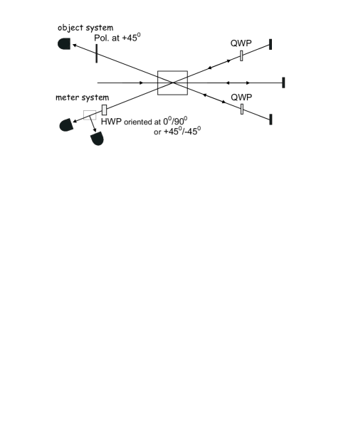
Figure 1: Here the setup for an active eraser is sketched. A bump beam transverses twice a e.g. type II crystal. The pairs produced in the first passage through the crystal cross two times a quarter–wave plate (QWP) which transforms an original horizontal polarized photon into a vertical one and vice versa. The pairs produced in the second passage through the crystal is directly directed to the measurement devices. The signal (object) photon is always measured after crossing a polarization analyzer aligned at $+45^{\circ}$. The idler (meter) photon crosses a half–wave plate (HWP) oriented at $0^{\circ},90^{\circ}$ (first setup) or $\pm 45^{\circ}$ (second setup) and is then analyzed by a polarization beam splitter. In the first setup —meter photon is measured in the $H/V$ basis— one has full which way information, namely if the pair was produced at the first or second passage. In the second setup —meter photon is measured in the $+45^{\circ}/-45^{\circ}$ basis— the information on the first or second passage is erased, one observes fringes or antifringes.

(b) Partially passive quantum eraser with active measurements

In Fig. 2 a setup is sketched where either at position A or B an entangled photon pair is produced, which was realized in Ref. Kim . “Clicks” on detector $D1$ or $D4$ provide “which way” information. “Clicks” on detector $D2$ and $D3$ give no information about the position A or B, interference is observed in the joint events of the two photons, see Fig. 2.

For kaons a piece of matter is permanently inserted into both beams where the one for the meter system at the right hand side is fixed at time $t_{r}^{0}$, see Fig. 3(b). The experiment observes the region from the source to the piece of matter at the right hand side. In this way the kaon moving to the right —the meter system— takes the choice to show “which width” information by its decay during its free propagation until $t_{r}^{0}$ or not by being absorbed in the piece of matter. Again strangeness or lifetime is measured actively. The choice whether the “wave–like” property or the “particle–like” property is observed is naturally given by the instability of the kaons. It is “partially active”, because the experimenter can choose at which fixed time $t_{r}^{0}$ the piece of matter is inserted. This is analogous to the optical case where the experimenter can choose the transmittivity of the two beam–splitters $BSA$ and $BSB$ in Fig. 2.

Furthermore, note that it is not necessary to identify $K_{S}$ versus $K_{L}$ for demonstrating the quantum marking and eraser principle.

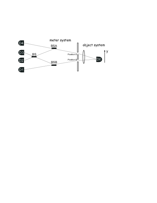
Figure 2: Here the setup of a partially active eraser is sketched. An entangled photon pair can be produced either in region $A$ or in region $B$. If the detectors $D1$ or $D2$ clicks, one knows the production region $A$ or $B$, i.e. one has full which way information. Clicks of the detectors $D2$ or $D3$ erase the information, interference is observed. It is a partially active eraser, because the mark is erased by a probabilistic law, however, the experimenter has still partially control over the erasure, she/he can choose the ratio of transmittivity to reflectivity of the beam splitter $BSA$ and $BSB$.

(c) Passive eraser with “passive” measurements on the meter

Next we consider the setup in Fig. 3(c). We take advantage —and this is specific for kaons— of the passive measurement. Again the strangeness content of the object system —kaon moving to the left hand side— is actively measured by inserting a piece of matter into the beam. In the beam of the meter no matter is placed in, the kaon moving to the right propagates freely in space. This corresponds to a passive measurement of either strangeness or lifetime on the meter by recording the different decay modes of neutral kaons. If a semileptonic decay mode is found, the strangeness content is measured. In the joint events interference is observed. If a two or three $\pi$ decay is observed, the lifetime is observed and thus “which width” information of the object system is obtained, no interference is seen in the joint events. Clearly we have a completely passive erasing operation on the meter, the experimenter has no control whether the lifetime mark is read out or not.

This experiment has no analog to any other considered two–level quantum system.

(d) Passive eraser with “passive” measurements

Finally we mention the setup in Fig. 3(d), where both kaons evolve freely in space and the experimenter observes passively their decay modes and times. The experimenter has no control over individual pairs neither on which of the two complementary observables at each kaon is measured nor when it is measured. This setup is totally symmetric, thus it is not clear which side plays the role of the meter and strictly speaking we cannot consider this experiment as a quantum eraser.

Kaonic quantum erasers

(a) Active eraser with active measurements (S: active/active; T: active)

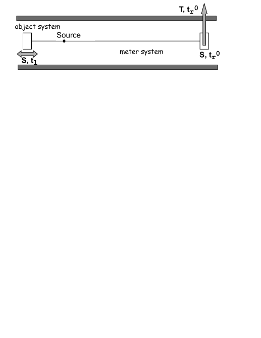
(b) Partially active eraser with active measurements (S: active/active; T: active)

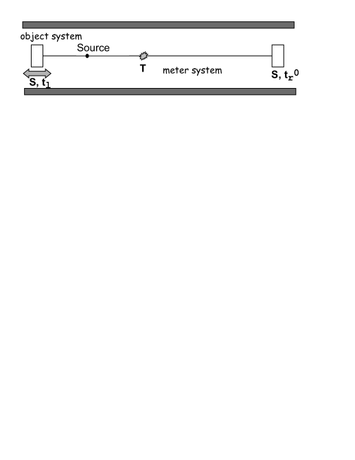
(c) Passive eraser with passive measurements on the meter (S: active/passive; T: passive)

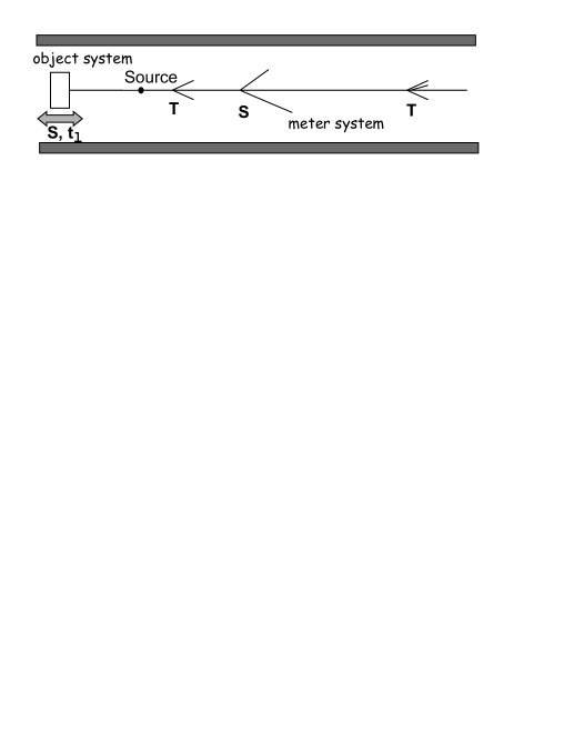
(d) Passive eraser with passive measurements (S: passive/passive; T: passive/passive)

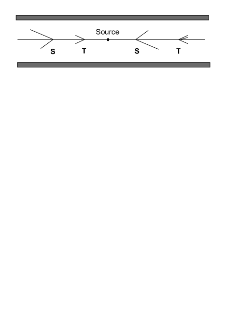
Figure 3: The figure shows four different setups for a quantum marking and quantum erasing experiment. The first three, (a), (b) and (c), have the object system on the left hand side on which the strangeness is always actively measured at time $t_{l}$. The setups (a) and (b) are analogous to existing quantum eraser experiments with entangled photons, see Fig. 1 and Fig. 2. The setup (c) has no analog, because only for kaons a passive measurement is possible. For the last setup, (d), it is not so clear which side plays the meter/object role as it is totally symmetric and it involves only passive measurements.

Summarizing, it is remarkable that for all four presented setups combining active and passive measurement procedures lead to the same observable probabilities! This is even true regardless of the temporal ordering of the measurements, thus kaonic erasers can also be operated in the “delayed choice” mode (for details see Ref. SBGH6 ).

VI Conclusions

In high energy physics neutral kaons —concerning their properties as quasi–spin— represent qubits, which we call kaonic qubits. However, there are important differences in comparison to photonic qubits. Kaons oscillate in strangeness, $K^{0}\leftrightarrow\bar{K}^{0}$, they decay and are characterized by $CP$ violation. Furthermore, kaon pairs also occur as entangled states in analogy to entangled photon pairs.

We construct a Bell inequality for quasi–spins. To our surprise, the premises of local realistic theories are only compatible with strict $CP$ conservation in the $K^{0}\bar{K}^{0}$ system. In this sense $CP$ violation is a manifestation of the nonlocality of the considered state!

We also want to remark that the considered Bell inequality, since it is chosen at time $t=0$, it is rather contextuality than nonlocality which is tested. Noncontextuality, the independence of the value of an observable on the experimental context due to its predetermination —a main hypothesis in hidden variable theories— is definitely ruled out! So the contextual quantum feature is demonstrated for entangled kaonic qubits.

However, kaons represent more than just qubit states. Due to the time evolution given by Nature kaons can be considered as double slits corresponding to the two different decay states, $|K_{S}\rangle,|K_{L}\rangle$. As time evolves both slits shrink, one faster than the other. The contrast of the strangeness oscillation corresponds to the visibility of the interference pattern and the “which width” information of the decay corresponds to the path predictability. With this interpretation the validity of the quantitative complementarity relation is perfectly demonstrated.

Finally, kaons are suitable systems to exhibit the amazing features of a quantum eraser. Compared to photons we can study even more, namely “active” and “passive” measurements, and this offers the possibility to prove new eraser concepts. Four possible setups are constructed, and remarkably all four —the active and passive measurements— lead to the same observable probabilities. This illustrates nicely the very nature of a quantum eraser experiment: it essentially sorts different events, namely, strangeness–strangeness or strangeness–lifetime events representing the “wave–like” or the “particle–like” property.

Kaon experiments verifying the proposed quantum marking and eraser procedures have not been performed till this day. Only the CPLEAR collaboration CPLEAR did part of the job required for the first setup of the active eraser.

Acknowledgement: The authors acknowledge financial support from EURIDICE HPRN-CT-2002-00311. We also would like to thank the referee for useful comments.

References

- (1) R.A. Bertlmann, “Entanglement, Bell inequalities and decoherence in particle physics”, Lecture Notes in Physics (Springer-Verlag, Berlin, 2005), quant-ph/0410028.
- (2) R. A. Bertlmann, B. C. Hiesmayr, Phys. Rev. A 63, 062112 (2001).
- (3) N. Gisin and A. Go, Am. J. Phys. 69, 264 (2001).
- (4) R.A. Bertlmann, A. Bramon, G. Garbarino and B.C. Hiesmayr, Phys. Lett. A 332, 355 (2004).
- (5) K. Nagata, W. Laskowski, M. Wieśniak and M. Żukowski, Phys. Rev. Lett. 93, 230403 (2004).
- (6) C.S. Unnikrishnan, Europhys. Lett. 69, 489 (2005).
- (7) F. Uchiyama, Phys. Lett. A 231, 295 (1997).
- (8) R.A. Bertlmann, W. Grimus and B.C. Hiesmayr, Phys. Lett. A 289, 21 (2001).
- (9) D.E. Groom et al, Review of Particle Physics, Eur. Phys. J. C 3, 1 (1998).
- (10) R.P. Feynman, R.B. Leighton and M. Sands, The Feynman Lectures on Physics, Vol. 3, (Addison-Wesley, 1965), p. 1-1, p. 11-20.
- (11) D. Greenberger and A. Yasin, Phys. Lett. A 128, 391 (1988).
- (12) B.-G. Englert, Phys. Rev. Lett. 77, 2154 (1996).
- (13) A. Bramon, G. Garbarino and B. C. Hiesmayr, Phys. Rev. A 69, 022112 (2004).
- (14) B.C. Hiesmayr and V. Vedral, “Interferometric wave-particle duality for thermodynamical systems”, quant-ph/0501015.
- (15) M. Arndt, O. Nairz, J. Vos-Andreae, C. Keller, G. Van der Zouw and A. Zeilinger, Nature 401, 680 682 (1999).
- (16) M. O. Scully and K. Drhl, Phys. Rev. A 25, 2208 (1982).
- (17) S. Drr and G. Rempe, Opt. Commun. 179, 323 (2000).
- (18) T.J. Herzog, P.G. Kwiat, H. Weinfurter and A. Zeilinger, Phys. Rev. Lett 75, 3034 (1995).
- (19) Y.-H. Kim, R. Yu, S.P. Kuklik, Y. Shih and M.O. Scully, Phys. Rev. Lett. 84, 1 (2000).
- (20) T. Tsegaye, G. Bjrk, M. Atatre, A.V. Sergienko, B.W.A. Saleh and M.C. Teich, Phys. Rev. A 62, 032106 (2000).
- (21) S.P. Walborn, M.O. Terra Cunha, S. Padua and C.H. Monken, Phys. Rev. A 65, 033818 (2002).
- (22) A. Trifonov, G. Bjrk, J. Sderholm and T. Tsegaye, Eur. Phys. J. D 18, 251 (2002).
- (23) H. Kim, J. Ko and T. Kim, Phys. Rev. A 67, 054102 (2003).
- (24) Y. Aharonov and M.S. Zubaiy, Science 307, 875 (2005).
- (25) A. Bramon, G. Garbarino and B. C. Hiesmayr, Phys. Rev. Lett. 92, 020405 (2004).
- (26) A. Bramon, G. Garbarino and B. C. Hiesmayr, Phys. Rev. A 68, 062111 (2004).
- (27) A. Apstolakis et.al., Phys. Lett. B 422, 339 (1998).