Dynamics beyond completely positive maps: some properties and applications

Abstract

Maps that are not completely positive (CP) are often useful to describe the dynamics of open systems. An apparent violation of complete positivity can occur because there are prior correlations of the principal system with the environment, or if the applied transformation is correlated with the state of the system. We provide a physically motivated definition of accessible non-CP maps and derive two necessary conditions for a map to be accessible. We also show that entanglement between the system and the environment is not necessary to generate a non-CP dynamics. We describe two simple approximations that may be sufficient for some problems in process tomography, and then outline what these methods may be able to tell us in other situations where non-CP dynamics naturally arise.

I Introduction

All real world systems interact to some extent with their environments, so they are said to be “open” open ; open2 ; open3 . When the initial correlations with the environment can be neglected the evolution is well-described by a completely positive map (CP-map). A CP-map can always be written in the Kraus form Kr83 ,

$$\rho^{\prime}=\Lambda(\rho)=\sum_{a}M_{a}\rho M^{\dagger}_{a}.$$ (1)

When the Kraus operators $M_{a}$ satisfy the completeness relation,

$$\sum_{a}M^{\dagger}_{a}M_{a}=\openone,$$ (2)

the map is also trace preserving, so that $\text{tr}\,\rho^{\prime}=\text{tr}\,\rho$.

However, if the system and the environment are initially correlated the resulting reduced dynamics may not be CP pech ; Al95 ; buz ; em1 ; jss ; ss05 . Positive but non-CP maps also play an important role in characterizing the phenomenon of quantum entanglement ppt ; H3 ; blin ; maj04 . Our goal is to investigate under what circumstances non-CP maps can describe an actual quantum dynamics and when (and if) the deviations from CP dynamics can be ignored.

To simplify the exposition we consider finite-dimensional systems. The combined state of a system ($A$) and its environment ($B$) can be represented in the Fano form Fa83

$$\tau_{AB} =\frac{1}{d_{A}d_{B}}\Bigl{(}\openone_{AB}+\sum_{i}\alpha_{i}\sigma^{A}_{i}\otimes\openone_{B}$$

$$+\sum_{j}\beta_{j}\openone_{A}\otimes\sigma^{B}_{j}+\sum_{ij}\gamma_{ij}\sigma^{A}_{i}\otimes\sigma^{B}_{j}\Bigr{)}.$$ (3)

Here the $\sigma_{i}^{A}$, $i=1,...,d_{A}^{2}$ represent generators of SU($d_{A}$), while the real vector $\vec{\alpha}$ of size $d_{A}^{2}-1$ is the generalized Bloch vector of the reduced density operator $\rho={\rm tr}_{B}\tau_{AB}$. Analogously, the $\sigma_{i}^{B}$ represent generators of SU($d_{B}$) and $\vec{\beta}$ of size $d_{B}^{2}-1$ denotes the generalized Bloch vector of the reduced density operator $\omega={\rm tr}_{A}\tau_{AB}$. The correlations between subsystems $A$ and $B$ are characterized by mah95

$$\Gamma_{ij}=(\gamma_{ij}-\alpha_{i}\beta_{j})/d_{A}d_{B}.$$ (4)

We assume that the overall evolution of $\tau_{AB}$ is unitary. To specify a non-unitary dynamics of the system $A$ we need to describe how it is embedded into a larger system $AB$. This is described by a map $E_{\mathcal{V}}$ such that,

$$\rho\to E_{\mathcal{V}}(\rho)=\tau,\qquad\text{tr}_{B}(\tau)=\rho,$$ (5)

which is called an assignment Al95 or an extension map jss . A tensor product assignment with a an initial $\omega^{0}$ that is independent of $\rho,$ on the auxiliary Hilbert space $\mathcal{H}_{B}$ followed by a unitary $U$ leads to a CP-map Kr83 ,

$$\rho^{\prime}=\text{tr}_{B}\bigl{(}U(\rho\otimes\omega^{0})U^{\dagger}\bigl{)}\ .$$ (6)

If the initial state of the environment $\omega$ is related to the initial state of the system $\rho,$ then the reduced evolution of the system may be non-linear. For example nonlin , $\rho$ may be an improper mixture (i.e., obtained by taking a partial trace from some larger system). This procedure yields an ensemble of pure states that depend on some classical parameter $c,$ $\psi_{A}(c)\otimes\psi_{B}(c).$ Alternatively, the marginal state of the environment may be independent of $\rho,$ but if the applied transformation $\Phi$ depends on some parameter $c,$ the final density matrix $\rho^{\prime}$ will not generally be equal to the result of applying the average of $\Phi$ over $c$ to $\rho$. This latter situation has arisen in the process tomography of a nuclear magnetic resonance quantum information processor em2 .

Part of the controversy surrounding non-CP maps in literature Al95 can be traced to ambiguities in the definitions of the extension maps. Moreover, the presence of correlations may blur the boundary between the system and its environment. The main aim of this work is to introduce a class of non-CP maps that may be useful in the description of the dynamics of open systems correlated with the environment and to analyze some of their properties.

The rest of this article is organized as follows. In the next section we provide a short review of some properties of positive linear maps. The notion of accessible maps is introduced in Section III while their properties are investigated in Section IV. Some implications for process tomography are presented in Section V and a few other applications of non-CP maps are discussed in Section VI.

II Maps and dynamical matrices

In this section we recall several properties of linear maps on the set of density matrices. A linear, hermiticity-preserving transformation $\Phi$ acting in the space of density matrices may be represented by the dynamical (Choi) matrix $D(\Phi)$ su61 ; choi ,

$$\rho^{\prime}_{mn}=\sum_{s,t}D_{ms;nt}\,\rho_{st},$$ (7)

which has a number of useful properties karol . The trace preserving condition (2) is equivalent to the following constraint on the partial trace of the dynamical matrix,

$$\sum_{m}D_{ms;mt}=\delta_{st}\ ,$$ (8)

which implies $\sum_{a}\lambda_{a}=d_{A}$. Moreover, if the map is unital, i.e., it maps the maximally mixed state into the maximally mixed state, then

$$\sum_{s}D_{ms,ns}=\delta_{mn}\ .$$ (9)

The dynamical matrix is Hermitian, $(D^{\dagger})_{ms;nt}=D^{*}_{nt;ms},$ and due to a theorem of Choi choi its positivity is equivalent to the complete positivity of $\Phi$. This property follows from the eigen-decomposition of the Choi matrix,

$$D_{ms;nt}=\sum_{a}\lambda_{a}(M_{a})_{ms}(M_{a}^{\dagger})_{tn}\ ,$$ (10)

in which all the eigenvalues $\lambda_{a}$ are non–negative.

If the dynamical matrix $D$ is not positive we can split its spectrum into positive and negative parts. This step allows us to represent a linear non–CP map as the difference of two CP maps, called the difference form choi ; jss ,

$$\rho^{\prime} =\Lambda_{+}(\rho)-\Lambda_{-}(\rho)$$ (11)

$$=\sum_{\lambda_{a}>0}\lambda_{a}M_{a}\rho M_{a}^{\dagger}+\sum_{\lambda_{a}<0}\lambda_{a}M_{a}\rho M_{a}^{\dagger},$$ (12)

where the maps $\Lambda_{\pm}$ are completely positive.

Completely positive maps have another important property: distinguishability of the set of states $(\rho_{1},\rho_{2},\ldots)$ does not improve under any CP map dist . For example, the trace distance between two density matrices does not increase under any CP map $\Lambda,$ $|\rho_{1}-\rho_{2}|_{1}\equiv{\rm tr}|\rho_{1}-\rho_{2}|\leq{\rm tr}|\Lambda(\rho_{1}-\rho_{2})|.$

Despite its definition as a mathematical tool, some matrix elements of $D$ have a direct experimental significance. For example, by a narrow-band laser resonant transition $Z\leftrightarrow Z^{\prime}$ in a nitrogen-vacancy (NV) center in diamond, the fluorescence intensity autocorrelation function $g^{(2)}(t)$ is $g^{(2)}(t)=D_{zz^{\prime};zz^{\prime}}/\rho_{z^{\prime}z^{\prime}}$, where $\rho_{z^{\prime}z^{\prime}}$ is the steady-state population of the fluorescent substate $Z^{\prime}$ niz .

III Maps and embeddings

A possibly non-linear and non-positive map $\Phi$ that describes a state transformation on $A$ may be considered physically accessible if $\Phi(\rho)=\text{tr}_{B}U\tau U^{\dagger}$, with the embedding described by some $E_{\mathcal{V}}$. The domain $\mathcal{V}$ of $\Phi$ should be a finite volume (i.e., non-empty) subset of the set of all states of $A,$ which we will call $\mathcal{M}_{A}.$ This is the first non-trivial requirement: physically relevant maps should be identifiable by process tomography, and convex combinations of a tomographically complete set of states must span a finite-volume region of $\mathcal{M}_{A}.$ In addition, a non-positive map $\Phi$ may only be accessible for states in its domain of positivity, where $\Phi(\rho)\geq 0.$

However, this definition is still too broad; some more restrictions on the assignment maps are essential. Without these further conditions the definition of accessibility remains trivial: any map becomes accessible on its domain of positivity. For example, the positive non-CP transposition map $T:\rho\mapsto\rho^{T}$, results from the extension $E(\rho)=\rho\otimes\rho^{T}$ followed by the SWAP gate, $U_{\text{SWAP}}(\rho\otimes\omega)U_{\text{SWAP}}^{\dagger}=\omega\otimes\rho$. An arbitrary non-linear map $\rho\mapsto\rho^{\text{final}}$ can be realized by $E(\rho)=\rho\otimes\rho^{\text{final}}$ and the unitary SWAP.

It might be objected that this construction is rather contrived. However, when we are setting the dials of our preparation apparatus in order to produce our tomographically complete set of input states, we are giving that apparatus a complete, classical description of the state we would like it to produce. Once we have done that, there is no a priori reason why the apparatus should not produce extra copies of the state, or ones that have undergone some peculiar map.

There is another way of demonstrating this point that draws on quantum information about the tomographically complete set of input states instead of the classical description of the state invoked above. Suppose instead that we are given that the environment consists of infinitely many copies of the state of the system (in a tensor product). Then the environment contains a complete (i.e., classical) description of the state, and can be used to implement an arbitrary map. This can be seen by noting that we could use the copies in the environment to do exact state tomography and then proceed as above RBK . There is also a direct equivalence between partial quantum information about a state (in the form of finitely many duplicate copies of that state) and incomplete or “fuzzy” classical descriptions of that state, via optimal state tomography.

Therefore we can implement any map that depends on detailed (classical) knowledge of the state provided we have access to an environment that contains a sufficiently large number of copies of that state. If the map requires knowledge of the state that is infinitely precise (i.e., in order to perform this map correctly, we must pick out a lower-dimensional subset of the set of density matrices) then an infinite number of copies in the environment would be required. For example, if we know what $\rho$ is exactly, we can always perform the map $\rho\mapsto\rho^{T}$ by another route: Find the unitary $U$ such that $U\rho U^{\dagger}$ is diagonal, and then do $UU\rho U^{\dagger}U^{\dagger}=\rho^{T}.$ However, this map depends on $\rho,$ via $U,$ and it requires exact knowledge of the eigenstates of $\rho.$ There are also other ways of using multiple copies of a state to perform exotic maps on that state.

We can draw a number of conclusions from these observations:

(i) if the ancilla system $\omega$ depends on $\rho,$ a non-CP map may arise from a tensor product assignment;
(ii) the domain $\mathcal{V}$ may be the entire set of states $\mathcal{M}_{A};$
(iii) Given enough copies of $\rho$ in the environment, any map can be performed RBK .

Clearly realistic systems will not have environments that contain so much information about the state that point (iii) becomes a completely unmanageable problem, but how much information is it reasonable to assume the environment might have about the state? The information known to the environment is part of the assignment map, thus our first task is to demarcate the set of physically reasonable assignment maps. We will begin by considering the simplest, “linear” case where the assignment map is linear; i.e., the marginal state of the environment $\omega$ is independent of $\rho$ and the correlations between system and environment can only be seen in the density matrix of the combined system $\tau_{AB}.$ We will then consider the slightly more general “affine” case, before discussing what approximations might be possible for the “non-linear” cases where $\omega$ is allowed to depend on $\rho$ directly.

III.1 The linear case

The simplest scenario is an initial value problem in which the time evolution of different initial states of the system is analyzed given that the initial state of the environment and the system-environment correlations are independent of $\rho.$ If the initial Bloch vector of the system is $\vec{\alpha},$ the $\beta_{j}$ could still depend on the $\alpha_{i}.$ If this is not the case (i.e., $\beta_{j}=b_{j},$ a constant) then we can write

$$\beta_{j}=b_{j},\qquad\gamma_{ij}=g_{ij}+\alpha_{i}b_{j}.$$ (13)

where $g_{ij}=d_{A}d_{B}\Gamma_{ij}.$ In general, $\Gamma_{ij}$ may depend on $\rho$ as well as the $\alpha_{i},$ but for the case when $g_{ij}$ is a constant matrix, $\gamma$ depends only on the $\alpha_{i},$ via the second term in (13).

Under the action of a unitary $U$ on the extended system, a useful form of the reduced dynamics of $\rho$ is obtained using the following procedure proposed by Štelmachovič and Bužek buz .

Decompose the extended density matrix $\tau_{AB}$ into a simple tensor product and the remaining term,

$$\tau_{AB}=\rho\otimes\omega+(\tau_{AB}-\rho\otimes\omega).$$ (14)

The direct product term yields a CP-map, as $\omega$ is independent of $\rho$ so this term is in Stinespring form. Using the spectral decomposition $\omega=\sum_{\nu}p_{\nu}|\nu\rangle\langle\nu|$ and writing the partial trace as

$$\text{tr}_{B}(U\rho\otimes\omega U^{\dagger})=\sum_{\mu,\nu}\langle\mu|\sqrt{p_{\nu}}\,U|\nu\rangle\rho_{A}\langle\nu|\sqrt{p_{\nu}}\,U^{\dagger}|\mu\rangle,$$ (15)

where the $|\mu\rangle$ form an orthonormal basis in $\mathcal{H}_{B},$ and defining $M_{\mu\nu}=\langle\mu|\sqrt{p_{\nu}}\,U|\nu\rangle,$ one obtains Eq. (1) after merging the double index $\mu\nu$ into a single index, $a.$ Hence the affine form of $\Phi(\rho)=\rho^{\prime}$ is given buz by

$$\Phi(\rho) ={\text{tr}}_{B}[U(E_{\mathcal{V}}(\rho))U^{\dagger}]$$

$$=\sum_{a}M_{a}\rho M_{a}^{\dagger}+\sum_{\mu}\sum_{i,j}\frac{g_{ij}}{d_{A}d_{B}}\langle\mu|U\sigma^{A}_{i}\otimes\sigma^{B}_{j}U^{\dagger}|\mu\rangle.$$ (16)

III.2 The affine case

The assumption that the initial environmental marginal $\omega^{0}$ cannot depend on the initial state $\rho^{0}$ is rather strong; for realistic (and poorly characterized) systems, we should not rule out any functional dependence a priori, thus we should treat $\omega^{0}=\omega^{0}(\rho^{0})$ unless we have good reason to assume the system does, in fact, behave like the linear case.

As noted above, if the environment has access to infinitely many copies of $\rho^{0},$ then any dynamical map can be induced on the system and the problem is intractable. However, that scenario is also rather unnatural. The question now becomes: can we make some physically well-motivated assumption about this system that will also make the problem tractable? We will make the assumption that although the environment “knows” something about the state, it only knows a little information. We believe that this is a plausible assumption to make for physically reasonable systems and we will proceed with our analysis on that basis.

In practice the state $\tau_{AB}$ may result from the evolution of $\rho^{0}\otimes\omega^{0}$ under some (imperfectly controlled) unitary $V$ which acts on the combined system. This can be a more realistic description of scenarios such as a gate being applied to a qubit that was stored in an imperfect quantum memory than a simple CP map. When the desired gate is eventually applied, the target state $\rho$ is only an approximation to the intended state $\rho^{0}.$ The dynamical matrix for the process $\rho^{0}\mapsto\rho$ is readily obtained as

$$D_{ac;bd}=\sum_{\alpha,\gamma,\delta}V_{a\alpha;c\gamma}V^{*}_{b\alpha,d\delta}\omega^{0}_{\gamma\delta}.$$ (17)

Likewise, the evolution of the environment is described by a similar expression, with the environment’s dynamical matrix depending on $\rho^{0}:$

$$D_{ac;bd}^{(E)}=\sum_{\alpha,\gamma,\delta}V_{a\alpha;c\gamma}V^{*}_{b\alpha,d\delta}\rho^{0}_{\gamma\delta}.$$ (18)

In generic cases $D$ describes a one-to-one mapping $\rho^{0}\mapsto\rho$ and therefore defines a unique transformation between the various coefficients. The values of the coefficients for the transformed matrix $\rho$ can be obtained by projection onto the original basis in the usual way:

$$\alpha_{i}={\rm tr}\sigma^{A}_{i}\rho,\qquad\beta_{j}={\rm tr}\sigma^{B}_{j}\omega,\qquad\gamma_{ij}={\rm tr}(\sigma_{i}^{A}\otimes\sigma_{j}^{B}\tau),$$ (19)

Inverting the transformation in Eq. (17) and using the dynamical matrix for the environment introduced in Eq. (18) above, we obtain the effective assignment map $\rho\mapsto\tau_{AB}$ with

$$\beta_{j}(\vec{\alpha})=\sum_{k}B_{jk}\alpha_{k},\qquad\gamma_{ij}(\vec{\alpha})=\sum_{k}G_{ijk}\alpha_{k},$$ (20)

with some constant coefficients $B_{jk}$ and $G_{ijk},$ which are independent of the $\alpha_{i}$ but do depend on $\beta_{0}.$

If $D$ is not a one-to-one map, then $\rho$ does not determine $\omega$ uniquely. Since all the relationships between the state parameters are linear, the effective assignment map in this case is given by

$$\beta_{j}^{\text{\,lin}}=b_{j}+\sum_{k}B_{jk}\alpha_{k},\qquad\gamma_{ij}^{\text{\,lin}}=g_{ij}+\sum_{k}G_{ijk}\alpha_{k},$$ (21)

which is actually the most general form of an affine assignment map, where the constants are subject to the positivity constraints, as before.

III.3 More general, non-linear cases…

An assignment map may also describe a preparation or be part of the specification of an imperfect quantum gate. In this case the correlation with the environment and/or its dependence on the state of the system are established either by design or accident, and the relations between $\rho$, $\omega$ and $\Gamma$ are potentially arbitrary. Allowing an arbitrary assignment map (even of the second degree) results in declaring all maps physically accessible, in principle, including perfect cloning, in a similar way to the transpose example above: $\rho\mapsto\rho^{\rm{final}}$. Of course, those examples do not exclude any functional forms of non-linear assignment maps. However, in practice the criteria for “reasonable” restrictions are rather ad hoc: while it is quite clear that the completely unconstrained case that allows perfect cloning should be excluded, the feasibility of less outlandish assignment maps is determined by the details of the actual physical system and the preparation methods. We leave those cases (like NMR em2 or NV-centre qubits ja ) for a later study. We discuss a particularly important example in in Section V.

Our discussion of the assignment maps can be summarized by the following definition.

Definition A map $\Phi$ defined by an assignment $E_{\mathcal{V}}(\rho)$ and a unitary $U,$

$$\Phi(\rho)={\text{tr}}_{B}[U(E_{\mathcal{V}}(\rho))U^{\dagger}]\ ,$$ (22)

is called affinely accessible if the assignment map satisfies the linearity conditions in Eq. (21) and the unitary $U$ does not depend on the initial state $\rho.$

IV Some properties of accessible maps

The affine form of a general linearly accessible map from Eq. (16) can be written

$$\Phi(\rho)=\sum_{a}M_{a}\rho M_{a}^{\dagger}+\sum_{\mu}\sum_{i,j}\Gamma_{ij}\langle\mu|U\sigma^{A}_{i}\otimes\sigma^{B}_{j}U^{\dagger}|\mu\rangle.$$ (23)

Since $\text{tr}\,U\sigma_{i}\otimes\sigma_{j}U^{\dagger}=\text{tr}\,\sigma_{i}\otimes\sigma_{j}=0,$ the inhomogeneous part is traceless and can be expressed as $\vec{\xi}\cdot\vec{\sigma}^{A}.$ The CP-map term is trace-preserving. Moreover, since the final state $\rho^{\prime}$ is Hermitian, all the coefficients $\xi_{i}$ are real. As a result, the dynamical matrix is given by

$$D_{ms;nt}=\sum_{\mu,\nu}(M_{\mu\nu})_{ms}(M_{\mu\nu})^{\dagger}_{nt}+\vec{\xi}\cdot\vec{\sigma}_{mn}\delta_{st}\,.$$ (24)

and the vector $\vec{\xi}\in{\mathbbm{R}}^{d_{A}^{2}-1}$ can be obtained by a comparison with Eq. (16).

If the building blocks of a non-CP map (namely, an extension map and a unitary evolution of the combined system) are linear and independent of the state $\rho,$ then the map $\Phi(\rho)$ is linear and the resulting dynamical matrix is independent of $\rho$. Indeed, it is easy to verify that $\Phi(c\rho_{1}+(1-c)\rho_{2})=c\Phi(\rho_{1})+(1-c)\Phi(\rho_{2})$. However, the affine form may still depend on the initial state of the combined system via the correlation tensor $\Gamma$ and/or $\omega$ and it will therefore appear non-linear (compare with dt99 ). In particular, a general assignment map of our example above, in Eq. (26) would lead to a quadratic dependence of $\Gamma_{ij}$ on $\rho$,

$$\Gamma_{ij}=\frac{1}{d_{A}d_{B}}(g_{ij}+\sum_{k}(G_{ijk}-\delta_{ik}b_{j})\alpha_{k}-\sum_{k}B_{jk}\alpha_{i}\alpha_{k}).$$ (25)

Another example of an assignment map is the extension $\tau_{AB}$ of a one-qubit mixed state, $\rho=\tfrac{1}{2}(\openone+\vec{\alpha}\cdot\vec{\sigma})$ to

$$\tau_{AB}=\frac{1}{4}\left[\openone_{AB}+\sum_{i=1}^{3}\alpha_{i}\sigma^{A}_{i}\otimes\openone_{B}+a\sum_{i=1}^{3}\sigma^{A}_{i}\otimes\sigma^{B}_{i}\right]\,.$$ (26)

The operator $\tau_{AB}$ is positive if

$$0\leq|a|\leq a_{\max}=(\sqrt{4-3|\alpha|^{2}}-1)/3.$$ (27)

Thus for any fixed $a,$ the domain $\mathcal{V}$ of the map $E$ is equal to the ball of radius $|\alpha|=\sqrt{(1+a)(1-3a)},$ centred on the maximally mixed state.

If the matrix $U$ commutes with the correlation term, which in our example means $[U,\sum_{i}\sigma_{i}^{A}\otimes\sigma_{i}^{B}]=0,$ the resulting map is trivially completely positive: the inhomogeneous part $\vec{\xi}\cdot\vec{\sigma}$ is zero nip .

Now consider the two-qubit unitary rotation,

$$U=\begin{pmatrix}1&0&0&0\\ 0&\cos\theta&\sin\theta&0\\ 0&-\sin\theta&\cos\theta&0\\ 0&0&0&1\end{pmatrix}.$$ (28)

The inhomogeneous part of the resulting $\Phi$ is now non-zero:

$$\vec{\xi}(a,\theta)\cdot\vec{\sigma}=\frac{1}{2}\begin{pmatrix}a\sin 2\theta&0\\ 0&-a\sin 2\theta\end{pmatrix},$$ (29)

however that alone is not enough to show that the map is non-CP. A typical situation is presented in Fig. 1, which shows the spectrum of the dynamical matrix as a function of the phase $\theta.$ The map $\Phi$ is not CP for some values of $\theta;$ for $\theta=\pi/4$ the affine form of $\Phi$ is merely an inconvenient way to write a CP map, whereas for $\theta=\pi$ the map is an accessible, genuinely non-CP transformation.

The conventional wisdom is that non-CP maps can only happen if the system is initially entangled with the ancilla. Our example consists of a two-qubit system and it is possible to detect entanglement using the positive partial transposition criterion ppt ; H3 . The results of this test show that the state $\tau$ is always classically correlated for $a>0$ (For $\alpha\leq 0$ the state $\tau$ may be entangled, e.g., the case $\alpha=0,a=-1/4$ corresponds to the triplet state $\Psi^{+}$). Moreover, even if $U(\theta)$ leads to a non-CP map, the state $U(\theta)\tau U^{\dagger}(\theta)$ is still unentangled.

Proposition 1. The existence of the affine form as in Eq. (16) with a trace-preserving completely positive map (that has at most linear dependence on $\rho$) and a traceless inhomogeneous part (that is at most quadratic, as in Eq. (25)) is a necessary condition for $\Phi$ to be accessible through a linear extension.

For a finite-dimensional ancilla the result follows from the definition of accessibility and Eq. (23). In the infinite-dimensional case we decompose a density operator $\tau_{AB}$ as in Eq. (14). After applying a unitary operation to $\tau_{AB}$ and taking the partial trace, the first term on the RHS yields a trace-preserving CP-map, and the second one is traceless and inhomogeneous. $\Box$

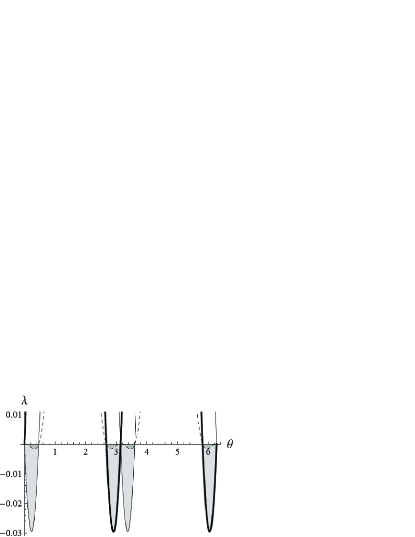
Figure 1: Three of the four eigenvalues of the dynamical matrix $D(\theta;a=0.2)$ become negative. Each line is one eigenvalue for a fixed value of $a=0.2$ and $\theta\in[0,2\pi].$

The conditions for Proposition 1 are non-trivial, as the next example shows. Consider the transposition of a qubit. Since it is a non-CP map, it has a difference form,

$$T(\rho)=\left(\sigma_{+}\rho\sigma_{+}+\sigma_{-}\rho\sigma_{-}+\sigma_{x}\rho\sigma_{x}/2\right)-(i\sigma_{y})\rho(i\sigma_{y})^{\dagger}/2,$$ (30)

where $\sigma_{\pm}=(\openone\pm\sigma_{z})/2.$ However, this map has no affine form and it is therefore not accessible, as we now demonstrate.

According to Proposition 1 the dynamical matrix of $D_{T}$ should be decomposable into a trace-preserving CP part $L(\vec{\xi})=\sum_{a}M_{a}\otimes M_{a}^{\dagger}$ and the inhomogeneous part $\vec{\xi}\cdot\vec{\sigma}\otimes\openone$, as in Eq.(24):

$$L(\vec{\xi})\equiv D-\vec{\xi}\cdot\vec{\sigma}\otimes\openone.$$ (31)

All the eigenvalues of $L(\vec{\xi})$ must be non-negative for $T(\rho)$ to be linearly accessible. However, a direct calculation shows that there is a negative eigenvalue $\lambda_{-}=-(1+\xi^{2})^{1/2},$ so $L$ is not positive for any $\vec{\xi},$ and thus is not linearly accessible. A non-linear realization with $E(\rho)=\rho\otimes\rho^{\text{T}}$ and $U=\mathrm{SWAP}$ can be written in the form $\rho^{\text{T}}=\sum_{a=1}^{4}M_{a}(\rho)\rho M_{a}(\rho)^{\dagger}$, but finding the matrices $M_{a}(\rho)$ requires a complete (i.e. classical) knowledge of the eigenbasis of $\rho.$

Moreover, it is interesting to note that a map

$$T^{\prime}\equiv p\Lambda_{\mathrm{dep}}+(1-p)T,\qquad 0\leq p\leq 1,$$ (32)

where $\Lambda_{\mathrm{dep}}(\rho)=\openone/2$ is the totally depolarizing channel, is linearly accessible only when it is actually CP, i.e., for $2/3\leq p\leq 1.$

Proposition 2. Any unital map that has a state-independent affine form is completely positive.

Any such map $\Phi$ has a form of Eq. (16). Following cn we decompose $\Lambda$ as

$$\Lambda(\rho)=\Lambda_{0}(\rho)+\vec{\varsigma}(\Lambda)\cdot\vec{\sigma},$$ (33)

where $\Lambda_{0}$ is a unital part of the map and $\vec{\varsigma}$ represents a translation of the generalized Bloch vector that depends only on the map $\Lambda$. The requirement $\Phi(\openone)=\openone$ implies $(\vec{\varsigma}+\vec{\xi})\cdot\vec{\sigma}=0,$ so $\Phi(\rho)=\Lambda_{0}(\rho)$ and $\Phi$ is a CP map. $\Box$

We note that this simple result can be immediately applied in the quantum causal histories approach to quantum gravity to reduce the number of independent axioms that characterize the dynamics of subsystems lt:07 .

V Some implications for process tomography

Imperfections in the preparation procedure may lead to non-linear correlations with the environment. If those correlations are sufficiently weak the assignment map may be written

$$\beta_{j}=\beta_{j}^{\text{\,lin}}+\varepsilon\beta_{j}^{1}(\vec{\alpha}),\quad\gamma_{ij}=\gamma_{ij}^{\text{\,lin}}+\varepsilon\gamma_{ij}^{1}(\vec{\alpha}),\quad\varepsilon\ll 1,$$ (34)

where $\beta_{j}^{1}$ and $\gamma_{ij}^{1}$ are arbitrary functions of $\vec{\alpha}$.

Consider now a weakly correlated and weakly interacting subsystems $A$ and $B$. Then the embedding $\rho\mapsto\tau$ is given by Eq. (34) with $\beta_{j}^{\text{\,lin}}=\beta_{j}^{0}$ and $\gamma_{ij}^{\text{\,lin}}=\alpha_{i}\beta^{0}_{j}$. As a result, the state of the environment is given by

$$\omega=\omega^{0}+\varepsilon\omega^{1}(\rho),\quad\text{tr}\,\omega^{1}=0,$$ (35)

and the system-environment correlations are described (to first order) by

$$\Gamma_{ij}=\varepsilon\Gamma_{ij}^{1}\equiv\frac{\varepsilon}{d_{A}d_{B}}(\gamma^{1}_{ij}-\alpha_{i}\beta_{j}^{1}).$$ (36)

When the system-environment interaction is weak,

$$H_{AB}=H_{A}\otimes\openone+\eta H_{\text{int}},\qquad\eta\ll 1,$$ (37)

where to simplify the notation we ignore the self-Hamiltonian of the environment. We also assume that the Hamiltonians are state-independent. The most general form of the Hamiltonian is

$$H_{A}=\sum_{i}h_{i}\sigma_{i}^{A},\qquad H_{\text{int}}=\sum_{ij}h_{ij}\sigma_{i}^{A}\otimes\sigma_{j}^{B}.$$ (38)

It is worth noting that the assignment map $\rho\mapsto\tau$ is non-linear at the first order of $\varepsilon$.

Proposition 3. At the first order of the perturbation theory in both the correlation strength and the interaction strength a reduced dynamics that results from the above assignment is linear and CP.

The unitary time-evolution operator is

$$U_{AB}=\exp(-it[H_{A}\otimes\openone+\eta H_{\mathrm{int}}]).$$ (39)

To leading order in $\eta$ it becomes

$$U_{AB} =U_{A}\otimes\openone_{B}(\openone_{AB}+\eta Q_{1}+\eta^{2}Q_{2}+\ldots)$$

$$\equiv U_{A}\otimes\openone_{B}+\eta O_{1}+\eta^{2}O_{2}+\ldots,$$ (40)

with

$$O_{1}\equiv-i\sum_{ij}\sum_{k=1}^{\infty}t^{k}c^{(k)}_{ij}U_{A}\sigma_{i}^{A}\otimes\sigma_{j}^{B},$$ (41)

where the coefficients $c^{(k)}_{ij}$ can be found using the Baker-Campbell-Hausdorff formula bch and SU($d_{B}$) commutation relations.

Assume for simplicity that $\rho_{B}^{0}$ has maximal rank and is non-degenerate. The Kraus matrices in the affine form of the reduced dynamics of Eq. (16) are independent of $\rho_{A}$ up to the second-order terms. Indeed,

$$M_{\mu\nu}\approx\langle\mu|(\sqrt{p^{0}_{\nu}}+\varepsilon p^{1}_{\nu}/2\sqrt{p^{0}_{\nu}})(U_{A}\otimes\openone+\eta O_{1})|\nu\rangle,$$ (42)

where $|\mu\rangle$ and $p^{0}_{\mu}$ are the unperturbed eigenvectors and eigenvalues, respectively, of $\omega^{0}$ and the indices $\mu\nu$ label the set of matrices, not the entries of a matrix. To first order we have

$$M_{\mu\nu}=\sqrt{p^{0}_{\nu}}U_{A}\delta_{\mu\nu}+\frac{\varepsilon p^{1}_{\nu}}{2\sqrt{p^{0}_{\nu}}}U_{A}\delta_{\mu\nu}+\eta\sqrt{p^{0}_{\nu}}\langle\mu|O_{1}|\nu\rangle.$$ (43)

When we substitute this expression into Eq. (1), the terms that are first order in $\varepsilon$ will cancel; thus (to first order) we can write

$$M_{\mu\nu}=M_{\mu\nu}^{0}+\eta\sqrt{p^{0}_{\nu}}\langle\mu|O_{1}|\nu\rangle,$$ (44)

where the matrices $M_{\mu\nu}^{0}$ form the Kraus representation of $U_{A}$. Next, the inhomogeneous part (as defined in Eq. (23))

$$\vec{\xi}\cdot\vec{\sigma}^{A}=\varepsilon\sum_{\mu}\sum_{i,j}\Gamma_{ij}^{1}\langle\mu|U_{AB}\sigma_{i}^{A}\otimes\sigma_{j}^{B}U_{AB}^{\dagger}|\nu\rangle,$$ (45)

is zero at the first order, because

$$\sum_{\mu}U_{A}\sigma_{i}^{A}U_{A}^{\dagger}\langle\mu|\sigma_{j}^{B}|\mu\rangle=0.$$ (46)

Hence at the first order of the perturbation theory the reduced evolution is still linear and CP. $\Box$

If $A$ is a cluster of qubits, $B$ is its environment and the reduced dynamics represents a physical realization of the perfect gate $U_{A}$, a high fidelity (of the actual outputs $\rho_{A}^{\rm{out}}$ with respect with to the ideal outputs $U_{A}|\psi_{A}^{\rm{in}}\rangle$) allows us to conclude that the first order perturbative expansion is valid. Hence Proposition 3 applies and the gate should be described by a CP map.

The raw tomographic data often yield non-positive dynamical matrices, which are usually considered unphysical ja ; james . A maximum-likelihood estimation or other such technique is used to convert the experimental data into a (positive) dynamical matrix james ; RBK . We see that this can be justified for characterizing actual high-fidelity implementations of “known” gates. However, when $\varepsilon$ and $\eta$ cannot be considered “small” a different template (such as a difference form) should be used to fit the data when attempting linear inversion process tomography.

VI Other applications

In this section we will examine a couple of other applications of induced dynamical maps that are non-CP.

VI.1 Dynamical decoupling

The preservation of quantum memory by dynamical decoupling from the environment viola clearly indicates that the reduced dynamics is non-CP. Let us revisit a simplified description of dynamical decoupling. Consider a system and the environment, initially in the state $\rho\otimes\omega$. Let the interaction Hamiltonian be $H_{AB},$ so the evolution in the interaction picture is given by $U=\exp(-iH_{AB}t).$ Assume that it is possible to produce a unitary map (such as an NMR pulse) $P=P_{A}\otimes{\openone}_{B}$ that anti-commutes with $H_{AB},$

$$PH_{AB}P^{\dagger}=-H_{AB}.$$ (47)

For example, if $H_{AB}=g\sigma_{z}^{A}\otimes O_{B},$ where $O_{B}$ is some operator that only acts on the environment and $g$ is a coupling constant, then $P_{A}=\sigma_{x}^{A}.$ The pulse sequence

$$Pe^{-iH_{AB}t}P^{\dagger}=U^{\dagger}$$ (48)

will reverse the original evolution $U$ provided that the pulse $P$ has negligible duration. Hence we will obtain $\rho(2t)=\rho(t=0).$

From the point of view of the system $A$ the above evolution appears to be an accessible (and possibly state-dependent) non-CP map. Let us assume for simplicity that the system is a single qubit parametrized by the Bloch vector, the environment is finite-dimensional and was originally in a completely mixed state. We will also assume that from the point of view of the environment alone, the evolution $U$ is a unital CP map, so $\omega(t)=\omega={\openone}/d_{B}.$ Then the evolution under $U$ of the initial state of $\rho\otimes{\mathbbm{1}}/d_{B}$ leads to

$$\tau_{AB}(t)=\frac{1}{2d_{B}}({\openone}_{AB}+\sum_{i,j}\alpha_{i}s^{i0}_{j0}\sigma^{A}_{j}\otimes\openone_{B}+\sum_{i,j,k}\alpha_{i}s^{i0}_{jk}\sigma_{j}^{A}\otimes\sigma_{k}^{B}),$$ (49)

where

$$U(\sigma^{A}_{\mu}\otimes\sigma^{B}_{\nu})U^{\dagger}=\sum_{\kappa\rho}s^{\mu\nu}_{\kappa\rho}\sigma^{A}_{\kappa}\otimes\sigma^{B}_{\rho}.$$ (50)

It is assumed here that the coefficients $s$ are time-dependent, the indices can take arbitrary integer values, $\mu=0,1,2,\ldots,$ and $j=1,2,\ldots,$ while the identity is denoted by $\sigma_{0}:=\openone.$ It is easy to see that the time-reversed evolution is given by a generalized inverse,

$$U^{\dagger}(\sigma^{A}_{\mu}\otimes\sigma^{B}_{\nu})U=c^{\mu\nu}_{\kappa\rho}\sigma^{A}_{\kappa}\otimes\sigma^{B}_{\rho},\quad\text{where}\quad c^{\mu\nu}_{\kappa\rho}s^{\kappa\rho}_{\zeta\eta}=\delta^{\mu}_{\zeta}\delta^{\rho}_{\eta}.$$ (51)

The state $\tau_{AB}(t)$ can be thought of as an image of a linear assignment map that was applied to

$$\rho(t)=\frac{1}{2}({\openone}_{A}+\alpha_{i}s^{i0}_{j0}\sigma^{A}_{j})$$ (52)

The pulses of Eq. (48) result in a non-CP map $\Phi$ that restores the state $\rho(t=0).$

VI.2 Quantum channels

A noisy quantum channel is usually modelled as a trace-preserving completely positive map. The information transmission from A(lice) to B(ob) can be then represented as an isometry between Alice’s Hilbert space and the Hilbert spaces of Bob and the environment,

$$V:{\cal{H}}_{A}\rightarrow{\cal{H}}_{B}\otimes{\cal{H}}_{C},$$ (53)

that is followed by a partial trace over the Hilbert space ${\cal{H}}_{C}$ (which is controlled by their colleague, Charlie). Several different channel capacities are defined, depending on the types of information and the resources that are at the disposal of the communicating parties. A typical message that is represented by a pure state $\psi\in{\cal{H}}$ is block-encoded by Alice (with a block size $n$) through the operation ${\cal{A}}:{\cal{H}}\rightarrow{\cal{H}}_{A}^{\otimes n}$ and is then sent through the channel, $V^{\otimes n}.$

Recently there has been some interest in the capacities of channels that are assisted by a “friendly” environment, which can measure states on ${\cal{H}}_{C}$ and communicate the result to Bob, thus potentially increasing one of the channel capacities friend . In these scenarios Charlie (who observes the environment) measures the environment before Bob attempts to recover the information. The measurement is described by a POVM ${E}_{x},$

$$E_{x}\geq 0,\qquad\sum_{x}E_{x}=\openone_{C}^{\otimes n},\vspace{-2mm}$$ (54)

on ${\cal{H}}_{C}^{\otimes n}$ and the outcome $x$ is communicated to Bob. The latter acts with the map ${\cal{R}}_{x}$ on his output, so the overall state transformation is given by

$${\Phi}(\psi)=\sum_{x}{\cal{R}}_{x}\!\left({\rm tr}_{C^{n}}[V^{\otimes n}{\cal{A}}(\psi)V^{\dagger\otimes n}({\mathbbm{1}}_{B}^{\otimes n}\!\otimes\!{{E}}_{x})]\right).$$ (55)

Such improvements in the distinguishability (and hence the capacity) show that from the point of view of the reduced states on ${\cal{H}}_{B},$ the overall procedure that starts with Charlie’s measurement and ends with ${\Phi}(\psi)$ must be non-CP.

In certain situations the process of encoding the “ideal” states (e.g., qubits) by Alice into the physical carriers may involve additional degrees of freedom. For example, when qubits are realized as a photon’s polarization and the finite size and spread of the wave packets is taken into account, the operations $\cal{A}$ and $V$ cannot be separated pho and the channel is not described by a CP map. Even in the absence of other sources of noise, continuous degrees of freedom can play the role of an environment, while a subsequent passage through lenses may lead to a non-CP evolution of the polarization degrees of freedom.

VII Open questions

The structure and applications of non-CP maps merit further investigation, particularly for the analysis of realistic quantum gates. While it was recently shown sud07 that for certain classes of extensions to separable states the reduced dynamics is always CP, there are still several important open questions. What conditions are sufficient for a map to be linearly accessible? What is the structure of the set of all linearly accessible maps? We have seen that the improvements in the distinguishability of quantum signals when the parties communicate, improvements in channel capacity or the preservation of quantum memory by dynamical decoupling from the environment are examples of non-CP maps. Their properties should be investigated in detail.

Another group of questions is related to following the reduced dynamics through time. A CP evolution forms a quantum dynamical semi-group and corresponds to a Lindblad-type master equation open ; open2 ; open3 . It is still an open question how a non-Markovian evolution is linked to non-CP maps open2 ; bre .

Acknowledgements

We have the pleasure of thanking Robin Blume-Kohout, Berthold-Georg Englert, Jens Eisert, Daniel James, Carlos Mochon, Debbie Leung, Daniel Lidar, Martin Plenio, Terry Rudolph, Barry Sanders, Jason Twamley and Shashank Virmani for stimulating discussions. HAC thanks iCORE and MITACS for financial support. DRT thanks the Institute for Mathematical Studies of the Imperial College for hospitality, and the Perimeter Institute for the great time he had there, and where the bulk of this work was done. KŻ is grateful to the Perimeter Institute for creating optimal working conditions in Waterloo and acknowledges support by grant number 1  P03B  042  26 from the Polish Ministry of Science and Information Technology and by the European Research project COCOS. The research at the Perimeter Institute is supported in part by the Government of Canada through NSERC and by the Province of Ontario through MRI.

References

- (1) R. Alicki and M. Fannes, Quantum Dynamical Systems, Oxford University Press, Oxford, 2001.
- (2) H.-P. Breuer and F. Petruccione, The Theory of Open Quantum Systems, Oxford University Press, New York, 2002).
- (3) F. Benatti and R. Floreanini, Int. J. Mod. Phys. B19, 3063 (2005).
- (4) K. Kraus, States, Effects and Operations: Fundamental Notions of Quantum Theory, Springer, Berlin, 1983.
- (5) P. Pechukas, Phys. Rev. Lett. 73, 1060 (1994).
- (6) R. Alicki, Phys. Rev. Lett. 75, 3020 (1995); P. Pechukas, Phys. Rev. Lett. 75, 3021 (1995)
- (7) P. Štelmachovič and V. Bužek, Phys. Rev. A 64, 062106 (2001).
- (8) N. Boulant, J. Emerson, T. F. Havel, D. G. Cory, and S. Furuta, J. Chem. Phys. 121, 2955 (2004).
- (9) T. F. Jordan, A. Shaji, and E. C. G. Sudarshan, Phys. Rev. A 70, 052110 (2004).
- (10) A. Shaji and E. C. G. Sudarshan, Physics Letters A 341, 48-54 (2005).
- (11) A. Peres, Phys. Rev. Lett. 77, 1413 (1996).
- (12) M., P., and R. Horodecki, Phys. Lett. A 223, 1 (1996).
- (13) B. M. Terhal, Linear Algebra Appl. 323, 61 (2000).
- (14) W. A. Majewski, Open Sys. & Information Dyn., 11 43-52 (2004).
- (15) U. Fano, Rev. Mod. Phys. 55, 855 (1983).
- (16) J. Schlienz and G. Mahler, Phys. Rev. A 52, 4396 (1995).
- (17) K. M. Fonseca Romero, P. Tolkner and P. Hänngi, Phys. Rev. A 69, 052109 (2004).
- (18) Y. S. Weinstein, T. F. Havel, J. Emerson, N. Boulant, M. Saraceno, S. Lloyd, and D. G. Cory, J. Chem. Phys. 121, 6117 (2004).
- (19) E. C. G. Sudarshan, P. M. Mathews and J. Rau, Phys. Rev. 121, 920 (1961).
- (20) M.-D. Choi, Linear Algebra Appl. 10, 285 (1975).
- (21) A. P. Nizovtsev, S. Ya. Kilin, F. Jelezko, I. Popa, A. Gruber, C. Tietz, and J. Wrachtrup, Optics and Spectroscopy 94, 848 (2003).
- (22) R. Blume-Kohout, private communication.
- (23) C. A. Fuchs and J. van de Graaf, IEEE Trans. Info. Theory IT-45, 1216 (1999).
- (24) I. Bengtsson and K. Życzkowski, Geometry of Quantum States, Cambridge University Press, Cambridge, 2006.
- (25) H. Hayashi, G. Kimura, and Y. Ota, Phys. Rev. A 67, 062109 (2003).
- (26) I. L. Chuang and M. A. Nielsen, J. Mod. Opt. 44, 2455 (1997).
- (27) D. R. Terno, Phys. Rev. A 59, 3320 (1999).
- (28) E. R. Livine and D. R. Terno, Phys. Rev. D 75, 084001 (2007).
- (29) D. F. V. James, P. G. Kwiat, W. J. Munro, and A. G. White, Phys. Rev. A 64, 052312 (2001); J. L. O’Brien, G. J. Pryde, A. Gilchrist, D. F. V. James, N. K. Langford, T. C. Ralph, and A. G. White, Phys Rev. Lett. 93, 080502 (2004).
- (30) M. Howard, J. Twamley, C. Wittmann, T. Gaebel, F. Jelezko and J. Wrachtrup, New J. Phys. 8, 33 (2006).
- (31) K. Goldberg, Duke Math. J. 23, 13 (1956); H. Kobayashi, N. Hatano, and M. Suzuki, Physica A 250, 535 (1998); M. W. Reinsch, J. Math. Phys. 41, 2434 (2000).
- (32) L. Viola and S. Lloyd, Phys. Rev. A 58, 2733 (1998); K. Khodjasteh and D. A. Lidar, Phys. Rev. Lett. 95, 180501 (2005).
- (33) M. Gregoratti and R. F. Werner, J. Mod. Opt. 50, 913 (2003); A. Winter, e-print quant-ph/0507045.
- (34) A. Peres and D. R. Terno, Rev. Mod. Phys. 76, 93 (2004).
- (35) A. Peres and D. R. Terno, J. Mod. Opt. 50, 1165 (2003); N. H. Lindner and D. R. Terno, J. Mod. Opt. 52, 1177 (2005).
- (36) C. Rodríguez, K. Modi, A. Kuah, E. C. G. Sudarshan, and A. Shaji, e-print quant-ph/0703022.
- (37) H. Breuer, Phys. Rev. A 75, 022103 (2007); A. A. Budini, Phys. Rev. A 74, 053815 (2006).